An Equivalence Theorem and A Sequential Algorithm for A-Optimal Experimental Designs on Manifolds

Abstract

Selecting input data points in the context of high-dimensional, nonlinear, and complex data in Riemannian space is challenging. While optimal experimental design theory is well-established in Euclidean space, its extension to Riemannian manifolds remains underexplored. Li and Del Castillo recently obtained new theoretical results on D-optimal and G-optimal designs on Riemannian manifolds. This paper follows their framework to investigate A-optimal designs on such manifolds. We prove an equivalence theorem for A-optimality under the manifold regularization model. Based on this result, a sequential algorithm for identifying A-optimal designs on manifold data is developed. Numerical studies using both synthetic and real datasets show the validity of the proposed method.

1. Introduction

Supervised learning models frequently rely on large labeled datasets to perform well, but labeling these datasets can be time-consuming and costly. A key challenge is how to select the most informative data points to improve model efficiency while minimizing labeling costs. This issue is closely related to the design of experiments (DOE), which focuses on selecting optimal designs based on some statistical criteria. In traditional DOE, it is often assumed that the statistical model is linear and the data lie on Euclidean space, with criteria usually focused on either parameter estimation or predictive performance (see Kiefer and Wolfowitz [1], Fedorov [2], Silvey [3], and Pukelsheim [4] for more details).

Modern tasks such as image recognition and text categorization often involve high-dimensional, nonlinear data. Manifold learning, or nonlinear dimensionality reduction, addresses these challenges by introducing the manifold structure. Basically, manifold learning assumes that although data reside in high-dimensional ambient spaces, they lie on lower-dimensional manifolds that offer a more compact representation (see, e.g., Roweis and Saul [5], Tenenbaum et al. [6], Donoho and Grimes [7], Coifman et al. [8], Belkin et al. [9]). Extensive research supports this assumption, showing that high-dimensional data are often sparse in ambient spaces, with most of the data concentrated on lower-dimensional manifolds. For a good review of existing manifold learning methods, see Meilă and Zhang [10]. Given this, traditional DOE methods, which rely on Euclidean assumptions, often fail to account for the complexities of such nonlinear data. Thus, optimal experimental design on manifolds, which considers the true underlying manifold structure, has become an essential tool in fields like biomedicine and computer vision. Manifold-based approaches enhance both the efficiency and accuracy of experiments, reducing labeling requirements while maximizing information gain.

While some previous studies have implemented optimal experimental design criteria as active learning strategies for high-dimensional data (e.g., He [11], Chen et al. [12], Alaeddini et al. [13]), these efforts lack theoretical justification for applying such designs on Riemannian manifolds. A pioneering study by Li and Del Castillo [14] explored D/G-optimal experimental designs on Riemannian manifolds, proving that D-optimal and G-optimal designs are equivalent in this context. They also proposed a lower bound for the maximum prediction variance and developed an efficient algorithm to find the optimal experimental design on manifold data.

While D-optimal designs are widely used due to their computational simplicity, A-optimal designs are still highly valuable, especially in situations where precise parameter estimation is crucial. Jones et al. [15] showed that A-optimal designs are generally preferred over D-optimal designs for early-stage experiments because they more directly align with the goal of identifying active factors by minimizing the average variance of parameter estimates, leading to better statistical properties, less collinearity, and improved prediction accuracy, especially when the two designs differ. These advantages become particularly evident in complex design spaces, where A-optimal designs lead to more stable optimization outcomes (Stallrich et al. [16]). Building on the above benefits, in this paper, we extend the framework of Li and Del Castillo [14] to investigate A-optimal designs on Riemannian manifolds. We prove an equivalence theorem for A-optimality under the manifold regularization model and propose a sequential algorithm to identify A-optimal experimental designs for manifold data. Numerical experiments on both synthetic and real datasets demonstrate the effectiveness of the proposed method.

The remainder of this paper is organized as follows. Section 2 reviews classical optimal experimental design in Euclidean space and the manifold regularization model from Belkin [9] and Li and Del Castillo [14]. Section 3 presents the main theoretical results, including the equivalence theorem for A-optimal designs on manifolds and a sequential algorithm. Section 4 provides numerical studies to validate the proposed methods. Section 5 concludes the paper with a summary and Section 6 provides some potential directions for future research. Additional simulation results are provided in the Supplementary Materials.

2. Preliminaries and Literature Review

2.1. Classical Optimal Experimental Design on Euclidean Space

The classical optimal experimental design theory on Euclidean space was introduced by Kiefer and Wolfowitz [1]. This framework uses optimization techniques to identify the optimal design that maximizes the efficiency of statistical inference under a given model. For a comprehensive treatment of optimal design theory, see Silvey [3] and Pukelsheim [4].

Consider the general linear regression model:

$$y=\sum _{j=1}^p{g}_j\left(\mathit{x}\right){\beta }_j+ϵ,$$

where $y\in \mathbb{R}$ is the response variable, $\mathit{x}={(x_1,\dots ,x_m)}^{\top }\in {\mathbb{R}}^m$ is the vector of input variables, $g_1,\dots ,g_p$ are known functions, $\mathsf{\beta }={({\beta }_1,\dots ,{\beta }_p)}^{\top }$ is the vector of unknown parameters, and $ϵ$ is a random error term, assumed to follow a normal distribution with mean 0 and variance ${\sigma }^2$.

Given a set of n design points ${\{{\mathit{x}}_i={(x_{i,1},\dots ,x_{i,m})}^{\top }\}}_{i=1,\dots ,n}$, suppose the corresponding response values are ${\left\{y_i\right\}}_{i=1,\dots ,n}$. The matrix form of the above model is

$$\mathit{y}=X\mathsf{\beta }+\mathsf{ϵ},$$

where $\mathit{y}={(y_1,\dots ,y_n)}^{\top }$,

$$X=\left[\begin{array}{ccc}{g}_1\left({\mathit{x}}_1\right)& \dots & g_p\left({\mathit{x}}_1\right)\\ ⋮& \ddots & ⋮\\ g_1\left({\mathit{x}}_n\right)& \dots & g_p\left({\mathit{x}}_n\right)\end{array}\right],$$

and $\mathsf{ϵ}={({ϵ}_1,\dots ,{ϵ}_n)}^{\top }$. The least squares estimate of $\mathsf{\beta }$ is given by

$$\widehat{\mathsf{\beta }}={\left(X^{\top }X\right)}^{-1}{X}^{\top }\mathit{y},$$

and the covariance matrix of $\widehat{\mathsf{\beta }}$ is

$$Cov(\widehat{\mathsf{\beta }})={\sigma }^2{\left(X^{\top }X\right)}^{-1}.$$

The Fisher information matrix for this linear regression model is $M=\frac{1}{n}{X}^{\top }X$.

In classical optimal design theory, exact designs are approximated by continuous designs, i.e., a probability measure with finite support points [3]. Let

$$\xi =\left\{\begin{array}{c}{\mathit{x}}_1,{\mathit{x}}_2,\dots ,{\mathit{x}}_{n_0}\\ q_1,q_2,\dots ,q_{n_0}\end{array}\right\},$$

where $q_i\ge 0$ and ${\sum }_{i=1}^{n_0}{q}_i=1$ denote a (continuous) design. The optimal design theory seeks to find the optimal design ${\xi }^{*}$ that optimizes a certain function of the Fisher information matrix, i.e.,

$${\xi }^{*}=arg\underset{\xi }{min}\Phi \left(M\left(\xi \right)\right),$$

where $\Phi (·)$ is the criterion function. Clearly, the optimal design ${\xi }^{*}$ depends on the specific optimality criterion $\Phi$. Numerous optimality criteria have been proposed in the literature, many of which are categorized as alphabetic optimality criteria, named after letters of the alphabet. Common criteria include D-optimality, where $\Phi \left(M\left(\xi \right)\right)={\left|M\left(\xi \right)\right|}^{-1}$, A-optimality, where $\Phi \left(M\left(\xi \right)\right)=tr\left(M{\left(\xi \right)}^{-1}\right)$, and G-optimality, where $\Phi \left(M\left(\xi \right)\right)={max}_{\mathit{x}}g{\left(\mathit{x}\right)}^{\top }M\left(\xi \right)g\left(\mathit{x}\right)$ with $g\left(\mathit{x}\right)={(g_1\left(\mathit{x}\right),\dots ,g_p\left(\mathit{x}\right))}^{\top }$. From a statistical perspective, D-optimal designs minimize the volume of the confidence ellipsoid for $\mathsf{\beta }$ [17]. A-optimal designs minimize the average of the variances of the parameter estimators, and G-optimal designs minimize the maximum prediction variance across the design region [3,4].

2.2. Manifold Learning and Manifold Regularization Model

Manifold learning is a form of dimensionality reduction that assumes the data distribution in high-dimensional space lies on a lower-dimensional manifold. The goal is to ensure that the reduced data preserve the geometric properties and structure inherent in the manifold of the high-dimensional space. Let $\mathcal{M}$ be a manifold in an m-dimensional space, a true subset of ${\mathbb{R}}^m$, i.e., $\mathcal{M}\subset {\mathbb{R}}^m$. Manifold learning aims to project this manifold onto a lower-dimensional space, such that $\mathcal{M}\to {\mathbb{R}}^n$ with $n\ll m$. This mapping aims to retain the intrinsic geometry of the manifold while reducing its dimensionality. Several well-known manifold dimensionality reduction algorithms, such as Locally Linear Embedding (LLE) and Isomap, have been proposed and extensively studied; see Roweis and Saul [5], Tenenbaum et al. [6], Donoho and Grimes [7], Coifman et al. [8], and Belkin et al. [9] for examples. For a recent comprehensive review, see Meilă and Zhang [10].

In contrast to conventional nonlinear dimensionality reduction methods, our work focuses on developing an optimal design methodology. We extend the framework proposed by Li and Del Castillo [14], which investigated D- and G-optimal designs in the manifold regularization model introduced by Belkin et al. [9]. Below, we briefly review the model setup; for technical details, see [14] and the references therein.

Let $\mathcal{X}\subset {\mathbb{R}}^d$ represent the input space and ${\left\{({\mathit{x}}_i,y_i)\right\}}_{i=1,\dots ,l}\subset \mathcal{X}\times \mathbb{R}$ the labeled training data. Let P be the joint distribution generating the labeled data, and $P_{\mathcal{X}}$ the marginal distribution that generates the unlabeled data ${\left\{{\mathit{x}}_i\right\}}_{l+1,\dots ,n}\subset \mathcal{X}$. In traditional machine learning, the goal is to learn a function $f:\mathcal{X}\to \mathbb{R}$ that maps instances to labels. Belkin et al. [9] extended this framework to Riemannian manifolds by assuming that the conditional distribution $P\left(y\right|\mathit{x})$ varies smoothly along the manifold supporting the data distribution $P_{\mathcal{X}}$. Specifically, if two points ${\mathit{x}}_1,{\mathit{x}}_2\in \mathcal{X}$ are close in geodesic distance, their label probabilities $P\left(y\right|{\mathit{x}}_1)$ and $P\left(y\right|{\mathit{x}}_2)$ are similar. They proposed a semi-supervised learning framework with a double-regularization objective function:

$$\widehat{f}=\underset{f\in {\mathcal{H}}_{\mathcal{K}}}{argmin}\left\{\sum _{i=1}^{l}V\left({\mathit{x}}_i,y_i,f\right)+{\lambda }_A{\parallel f\parallel }_{{\mathcal{H}}_{\mathcal{K}}}^2+{\lambda }_I{\parallel f\parallel }_I^2\right\},$$

(1)

where V is a known loss function, ${\mathcal{H}}_{\mathcal{K}}$ is a Hilbert space with a Mercer kernel $\mathcal{K}$, ${\parallel f\parallel }_{{\mathcal{H}}_{\mathcal{K}}}^2$ and ${\lambda }_A$ represent the non-smoothness penalty term and penalty quantity in the ambient space, respectively. The term ${\parallel f\parallel }_I^2$ penalizes the non-smoothness of f along the geodesics of the intrinsic manifold, ensuring that the learned function aligns more closely with the underlying data distribution, while ${\lambda }_I$ is the corresponding penalty weight for the manifold’s intrinsic geometry.

The penalty term ${\parallel f\parallel }_I^2$ serves as a roughness penalty related to the distribution $P_{\mathcal{X}}$ on the manifold. To illustrate this, consider a specific case where M, the support of $P_{\mathcal{X}}$, is a compact manifold. Then, we can define ${\parallel f\parallel }_I^2$ as

$${\int }_{x\in \mathcal{M}}{∥{\nabla }_{\mathcal{M}}f∥}^{2}d{P}_{\mathcal{X}}={\int }_{x\in \mathcal{M}}f{\Delta }_{\mathcal{M}}{f}^{\top }d{P}_{\mathcal{X}},$$

where ${\nabla }_{\mathcal{M}}$ is the gradient of f along the manifold $\mathcal{M}$, and ${\Delta }_{\mathcal{M}}$ is the Laplace–Beltrami operator. In most real-world applications, however, the distribution $P_{\mathcal{X}}$ is unknown, and one can replace it with an empirical estimate of the marginal distribution. Significant work has focused on scenarios where $P_{\mathcal{X}}$ is supported on a compact manifold $\mathcal{M}\subset {\mathbb{R}}^p$, and a finite set of points is used to infer the manifold structure (Roweis and Saul [5], Tenenbaum et al. [6], Donoho and Grimes [7], and Coifman et al. [8]). Given these assumptions, it has been demonstrated (see, for instance, Belkin [18]) that the problem (1) can be reformulated as

$$\widehat{f}=\underset{f\in {\mathcal{H}}_{\mathcal{K}}}{argmin}\left\{\sum _{i=1}^{l}V\left({\mathit{x}}_i,y_i,f\right)+{\lambda }_A{\parallel f\parallel }_{{\mathcal{H}}_{\mathcal{K}}}^2+{\lambda }_I{\mathbf{f}}^{\top }L\mathbf{f}\right\},$$

(2)

where $\mathbf{f}={[f\left(x_1\right),\dots ,f\left(x_n\right)]}^{\top }$ is the vector of function values at the data points, and L is the Laplacian matrix associated with the graph $\mathcal{G}$ that is constructed from the labeled and unlabeled data points ${\left\{{\mathit{x}}_i\right\}}_{i=1,\dots ,n}$. The graph Laplacian matrix L encodes the connectivity relationships among the data points and serves as an approximation to the Laplace–Beltrami operator on the continuous manifold $\mathcal{M}$.

The infinite-dimensional problem in Equation (2) can be reformulated as a finite sum over the labeled and unlabeled points, as follows:

$$f\left(\mathit{x}\right)=\sum _{i=1}^n{\alpha }_{i}K\left({\mathit{x}}_i,\mathit{x}\right),$$

(3)

where K is the Mercer kernel associated with the ambient space ${\mathcal{H}}_{\mathcal{K}}$. Denote $\mathsf{\alpha }={[{\alpha }_1,\dots ,{\alpha }_n]}^{\top }$ as the vector of parameters ${\alpha }_i$. The representer formula in (3) enables the derivation of a specific expression for the parameter estimates.

To discuss the optimal experimental design for the manifold regularization model (2), we consider a sequential experimental design problem, beginning with no labeled data. Let the set of labeled points at the k-th iteration be denoted as ${\left\{{\mathit{z}}_i\right\}}_{i=1}^k\subset {\left\{{\mathit{x}}_i\right\}}_{i=1}^n$, and the vector of their corresponding response values as $\mathit{y}={(y_1,\dots ,y_k)}^{\top }$.

To simplify, we adopt the setting in Li and Del Castillo [14] for the choice of ${\parallel f\parallel }_{{\mathcal{H}}_{\mathcal{K}}}^2$ and V in (2), where the squared loss function is used for V, and the RKHS space ${\mathcal{H}}_{\mathcal{K}}$ with $L_2$ norm is chosen for ${\parallel f\parallel }_{{\mathcal{H}}_{\mathcal{K}}}^2$. This leads to the Laplacian Regularized Least Squares (LapRLS) problem (Belkin [18]):

$$\widehat{f}=\underset{f\in {\mathcal{H}}_{\mathcal{K}}}{argmin}\left\{\sum _{i=1}^k{\left(y_i-f\left({\mathit{z}}_i\right)\right)}^2+{\lambda }_A{\parallel f\parallel }_{{\mathcal{H}}_{\mathcal{K}}}^2+{\lambda }_I{\mathbf{f}}^{\top }L\mathbf{f}\right\}.$$

(4)

By substituting the finite sum from Equation (3), i.e., $f\left(\mathit{x}\right)={\sum }_{i=1}^n{\alpha }_{i}K\left({\mathit{x}}_i,\mathit{x}\right)$, into Equation (4), we obtain the objective function for estimating the parameters $\mathsf{\alpha }$:

$$\widehat{\mathsf{\alpha }}=\underset{\mathsf{\alpha }\in {\mathbb{R}}^n}{argmin}\left\{{\left(\mathit{y}-K_{XZ}^{\top }\mathsf{\alpha }\right)}^{\top }\left(\mathit{y}-K_{XZ}^{\top }\mathsf{\alpha }\right)+{\lambda }_A{\mathsf{\alpha }}^{\top }K\mathsf{\alpha }+{\lambda }_I{\mathsf{\alpha }}^{\top }KLK\mathsf{\alpha }\right\},$$

(5)

where

$$\begin{array}{cc}\hfill K_{XZ}& ={\left[\begin{array}{ccc}\mathcal{K}\left({\mathit{x}}_1,{\mathit{z}}_1\right)& \dots & \mathcal{K}\left({\mathit{x}}_1,{\mathit{z}}_k\right)\\ ⋮& \ddots & ⋮\\ \mathcal{K}\left({\mathit{x}}_n,{\mathit{z}}_1\right)& \dots & \mathcal{K}\left({\mathit{x}}_n,{\mathit{z}}_k\right)\end{array}\right]}_{n\times k},\hfill \end{array}$$

and

$$\begin{array}{cc}\hfill K& ={\left[\begin{array}{ccc}\mathcal{K}\left({\mathit{x}}_1,{\mathit{x}}_1\right)& \dots & \mathcal{K}\left({\mathit{x}}_1,{\mathit{x}}_n\right)\\ ⋮& \ddots & ⋮\\ \mathcal{K}\left({\mathit{x}}_n,{\mathit{x}}_1\right)& \dots & \mathcal{K}\left({\mathit{x}}_n,{\mathit{x}}_n\right)\end{array}\right]}_{n\times n}.\hfill \end{array}$$

Taking the derivative of Equation (5) with respect to $\mathsf{\alpha }$ and letting it equal to zero gives

$$\widehat{\mathsf{\alpha }}={(K_{XZ}{K}_{XZ}^{\top }+{\lambda }_{A}K+{\lambda }_{I}KLK)}^{-1}{K}_{X}Z\mathit{y}.$$

To study optimal design theory, we further consider a linear model and a linear kernel for ${\mathcal{H}}_K$ without loss of generality. Then, the model parameters $\mathsf{\beta }$ can be estimated as follows:

$$\begin{array}{cc}\hfill \widehat{\mathsf{\beta }}& =X^{\top }\widehat{\mathsf{\alpha }}\hfill \\ \hfill & =X^{\top }{\left(X{Z}_k^{\top }{Z}_k{X}^{\top }+{\lambda }_{A}X{X}^{\top }+{\lambda }_{I}X{X}^{\top }LX{X}^{\top }\right)}^{-1}X{Z}_k^{\top }\mathbf{y}\hfill \\ \hfill & ={\left(Z_k^{\top }{Z}_k+{\lambda }_A{I}_p+{\lambda }_I{X}^{\top }LX\right)}^{-1}{Z}_k^{\top }\mathit{y},\hfill \end{array}$$

(6)

where

$$Z_k=\left[\begin{array}{c}g{\left({\mathit{z}}_1\right)}^{\top }\\ ⋮\\ g{\left({\mathit{z}}_k\right)}^{\top }\end{array}\right],X=\left[\begin{array}{c}g{\left({\mathit{x}}_1\right)}^{\top }\\ ⋮\\ g{\left({\mathit{x}}_n\right)}^{\top }\end{array}\right],\mathit{y}=\left[\begin{array}{c}{y}_1\\ ⋮\\ y_k\end{array}\right],$$

(7)

and $g\left(\mathit{x}\right)=(g_1\left(\mathit{x}\right),\dots ,g_p\left(\mathit{x}\right))$. Note that in this case, the model is linear in the parameters $\mathsf{\beta }$, though the function $g\left(\mathit{x}\right)$ is generally nonlinear in $\mathit{x}$.

As shown by He [11], since the regularization parameters ${\lambda }_A$ and ${\lambda }_I$ are typically small, we can approximate the covariance matrix of the parameter estimates in the following way [14]:

$$cov\left(\widehat{\mathsf{\beta }}\right)\approx {\sigma }^2{\left(Z_k^{\top }{Z}_k+{\lambda }_A{I}_p+{\lambda }_I{X}^{\top }LX\right)}^{-1}.$$

(8)

This equation provides a formula for the information matrix, which is essential for studying optimal design.

3. Main Results

3.1. The A-Optimality Criterion

Consider an infinite set of points $\mathit{x}$ uniformly distributed on a Riemannian manifold $\mathcal{M}\subset {\mathbb{R}}^d$. Let $\xi$ represent a (continuous) design (i.e., a  probability measure) on $\mathcal{M}$ with finite support, given by

$$\xi =\left\{\begin{array}{c}{\mathit{z}}_1,{\mathit{z}}_2,\dots ,{\mathit{z}}_{n_0}\\ q_1,q_2,\dots ,q_{n_0}\end{array}\right\},$$

where $\mathit{z}\in \mathcal{M}$, $q_i\ge 0$ and ${\sum }_{i=1}^{n_0}{q}_i=1$. Here, $\xi \left({\mathit{z}}_i\right)=q_i$ indicates that the proportion of experimental effort allocated to the point $z_i$ is $q_i$.

By Equation (8), for any design $\xi$, the information matrix for the LapRLS model (4) can be defined as

$$\begin{array}{cc}\hfill M_{\mathrm{Lap}}\left(\xi \right)=& {\int }_{\mathit{z}\in \mathcal{X}}\xi \left(\mathit{z}\right)g\left(\mathit{z}\right)g{\left(\mathit{z}\right)}^{\top }d\mathit{z}+{\lambda }_A{I}_p\hfill \\ \hfill & +{\lambda }_I{\int }_{x\in \mathcal{M}}g\left(\mathit{x}\right){\Delta }_{\mathcal{M}}g{\left(\mathit{x}\right)}^{\top }d\mu ,\hfill \end{array}$$

(9)

where $\mathcal{X}\subseteq \mathcal{M}$ is the experimental region on the manifold $\mathcal{M}$ and $\mu$ is the uniform measure on $\mathcal{M}$. Since the last two terms in the information matrix depend only on the overall manifold structure and not on the selected dataset, we introduce the following simplification for convenience:

$$C={\lambda }_A{I}_p+{\lambda }_I{\int }_{\mathit{x}\in \mathcal{M}}g\left(\mathit{x}\right){\Delta }_{\mathcal{M}}g{\left(\mathit{x}\right)}^{\top }d\mu .$$

By substituting the expression for C into Equation (9), the equation simplifies as follows:

$$M_{\mathrm{Lap}}\left(\xi \right)={\int }_{\mathit{z}\in \mathcal{X}}\xi \left(\mathit{z}\right)g\left(\mathit{z}\right)g{\left(\mathit{z}\right)}^{\top }d\mathit{z}+C.$$

(10)

We can now define the A-optimality criterion under the LapRLS model on manifolds. An experimental design ${\xi }^{*}$ is said to be A-optimal under LapRLS model (4) if it minimizes the trace of the inverse of the information matrix, i.e.,

$${\xi }^{*}=arg\underset{\xi }{min}\mathrm{tr}\left(M_{\mathrm{Lap}}^{-1}\left(\xi \right)\right),$$

where the information matrix $M_{\mathrm{Lap}}\left(\xi \right)$ is given by Equation (10). Similar to the statistical meaning of A-optimal designs on Euclidean spaces, an A-optimal design under the LapRLS model (4) minimizes the sum or average of the variances of the parameter estimators $\widehat{\mathsf{\beta }}$, as seen by Equation (8).

3.2. Equivalence Theorem for A-Optimal Designs on Manifolds

Before proving the equivalence theorem for A-optimal designs under the LapRLS model on manifolds, we first present the following lemma (Proposition 1 in [14]), which establishes the linearity property of the information matrix.

Lemma 1. 

The information matrix $M_{\mathrm{Lap}}(·)$ is linear with respect to the convex combination of experimental designs. Specifically, for any two designs ${\xi }_1$ and ${\xi }_2$ on $\mathcal{M}$, and for any $0<\alpha <1$, the following holds:

$$M_{\mathrm{Lap}}\left({\xi }_3\right)=(1-\alpha )M_{\mathrm{Lap}}\left({\xi }_1\right)+\alpha M_{\mathrm{Lap}}\left({\xi }_2\right),$$

where ${\xi }_3=(1-\alpha ){\xi }_1+\alpha {\xi }_2$ is the convex combination of ${\xi }_1$ and ${\xi }_2$.

Fedorov [2] established the equivalence theorem for classical linear optimality criteria in Euclidean spaces. We now adapt his approach to prove an equivalence theorem for A-optimal designs under the LapRLS model on manifolds.

It is well-known that the trace function $\mathrm{tr}(·)$ satisfies the following properties:

$$\begin{array}{cc}& \mathrm{tr}(A+B)=\mathrm{tr}\left(A\right)+\mathrm{tr}\left(B\right),\hfill \\ & \mathrm{tr}\left(kA\right)=k\mathrm{tr}\left(A\right),\hfill \\ & \mathrm{tr}\left(A\right)\ge 0,\hfill \end{array}$$

where A and B are positive semidefinite matrices. Now, consider the matrix

$$A=(1-\alpha )A_1+\alpha A_2,$$

where $0\le \alpha \le 1$, and $A_1$ and $A_2$ are positive semidefinite matrices. It is known that

$$A^{-1}\le (1-\alpha )A_1^{-1}+\alpha A_2^{-1},$$

where the matrix inequality implies a positive semidefinite relationship (i.e., $A\le B$ means $B-A$ is positive semidefinite). By applying the trace function to both sides of the inequality, we get

$$\mathrm{tr}\left(A^{-1}\right)\le (1-\alpha )\mathrm{tr}\left(A_1^{-1}\right)+\alpha \mathrm{tr}\left(A_2^{-1}\right),$$

which shows that $\mathrm{tr}\left[A^{-1}\right]$ is a convex function of A for a convex set of positive semidefinite matrices.

Using these properties and Lemma 1, we can derive the following equivalence theorem for A-optimal designs under the LapRLS model on manifolds.

Theorem 1. 

(Equivalence Theorem of A-Optimality on Manifolds) The following statements are equivalent:

(1) 

The experimental design ${\xi }^{*}$ is A-optimal under the LapRLS model (4), i.e., ${\xi }^{*}$ minimizes $tr\left(M_{\mathrm{Lap}}^{-1}\left(\xi \right)\right)$;

(2) 

The experimental design ${\xi }^{*}$ minimizes

$$\underset{\mathit{z}\in \mathcal{X}}{sup}tr\left\{M_{\mathrm{Lap}}^{-1}\left(\xi \right)\left[g\left(\mathit{z}\right)g{\left(\mathit{z}\right)}^{\top }+C\right]M_{\mathrm{Lap}}^{-1}\left(\xi \right)\right\};$$

(3) 

${sup}_{\mathit{z}\in \mathcal{X}}tr\left\{M_{\mathrm{Lap}}^{-1}\left({\xi }^{*}\right)\left[g\left(\mathit{z}\right)g{\left(\mathit{z}\right)}^{\top }+C\right]M_{\mathrm{Lap}}^{-1}\left({\xi }^{*}\right)\right\}=tr\left(M_{\mathrm{Lap}}^{-1}\left({\xi }^{*}\right)\right)$;

where the information matrix $M_{\mathrm{Lap}}\left(\xi \right)$ is defined in Equation (10).

Proof. 

(i) Proof of (1) ⇒ (2) and (3).

Let ${\xi }^{*}$ be the design that minimizes $\mathrm{tr}\left(M_{\mathrm{Lap}}^{-1}\left(\xi \right)\right)$, and let $\xi$ be an arbitrary design, not necessarily optimal. Define the new design ${\xi }^0$ as a convex combination of ${\xi }^{*}$ and $\xi$:

$${\xi }^0=(1-\alpha ){\xi }^{*}+\alpha \xi ,$$

where $0\le \alpha \le 1$.

By Lemma 1, the information matrix for ${\xi }^0$ is a convex combination of the information matrices for ${\xi }^{*}$ and $\xi$:

$$M_{\mathrm{Lap}}\left({\xi }^0\right)=(1-\alpha )M_{\mathrm{Lap}}\left({\xi }^{*}\right)+\alpha M_{\mathrm{Lap}}\left(\xi \right).$$

Since ${\xi }^{*}$ minimizes $\mathrm{tr}\left(M_{\mathrm{Lap}}^{-1}\left(\xi \right)\right)$, this minimality can be expressed in terms of derivatives. Differentiating $M_{\mathrm{Lap}}^{-1}\left(\xi \right)$ with respect to $\alpha$ and simplifying the notation by using M instead of $M_{\mathrm{Lap}}$, we get

$${\displaystyle \frac{\partial M^{-1}\left({\xi }^0\right)}{\partial \alpha }}=-M^{-1}\left({\xi }^0\right)\left[M\left(\xi \right)-M\left({\xi }^{*}\right)\right]M^{-1}\left({\xi }^0\right).$$

When $\alpha =0$, we have ${\xi }^0={\xi }^{*}$. Using the convexity of $\mathrm{tr}\left(M_{\mathrm{Lap}}^{-1}\left(\xi \right)\right)$, we can conclude that

$${\left.{\displaystyle \frac{\partial \mathrm{tr}\left(M^{-1}\left({\xi }^0\right)\right)}{\partial \alpha }}\right|}_{\alpha =0}=-\mathrm{tr}\left\{M^{-1}\left({\xi }^{*}\right)\left[M\left(\xi \right)-M\left({\xi }^{*}\right)\right]M^{-1}\left({\xi }^{*}\right)\right\}\ge 0.$$

Now, assume without loss of generality that the design $\xi$ consists of only a single point $\mathit{z}\in \mathcal{X}$. Substituting the information matrix of this singleton set into the above equation, we obtain

$$-\mathrm{tr}\left\{M^{-1}\left({\xi }^{*}\right)\left[g\left(\mathit{z}\right)g^{\top }\left(\mathit{z}\right)+C-M\left({\xi }^{*}\right)\right]M^{-1}\left({\xi }^{*}\right)\right\}\ge 0.$$

Rearranging the terms leads to

$$\mathrm{tr}\left\{M^{-1}\left({\xi }^{*}\right)\left[g\left(\mathit{z}\right)g^{\top }\left(\mathit{z}\right)+C\right]M^{-1}\left({\xi }^{*}\right)\right\}\le \mathrm{tr}\left(M^{-1}\left({\xi }^{*}\right)\right).$$

(11)

Next, we decompose the information matrix for any design $\xi$ and apply the properties of the trace function and the interchangeability of integration and summation:

$$\begin{array}{cc}\hfill \mathrm{tr}\left(M^{-1}\left(\xi \right)\right)& =\mathrm{tr}\left(M^{-1}\left(\xi \right)M\left(\xi \right)M^{-1}\left(\xi \right)\right)\hfill \\ & =\mathrm{tr}\left[M^{-1}\left(\xi \right)\left(\int \xi \left(\mathit{z}\right)g\left(\mathit{z}\right)g^{\top }\left(\mathit{z}\right)d\mathit{z}+C\right)M^{-1}\left(\xi \right)\right]\hfill \\ & =\mathrm{tr}\left[M^{-1}\left(\xi \right)\int \xi \left(\mathit{z}\right)g\left(\mathit{z}\right)g^{\top }\left(\mathit{z}\right)M^{-1}\left(\xi \right)d\mathit{z}+M^{-1}\left(\xi \right)C{M}^{-1}\left(\xi \right)\right]\hfill \\ & =\int \xi \left(\mathit{z}\right)\mathrm{tr}\left\{g^{\top }\left(\mathit{z}\right)M^{-1}\left(\xi \right)g\left(\mathit{z}\right)\right\}{M}^{-1}\left(\xi \right)d\mathit{z}+\mathrm{tr}\left(M^{-1}\left(\xi \right)C{M}^{-1}\left(\xi \right)\right).\hfill \end{array}$$

Using the form above, we derive the following inequality:

$$\begin{array}{cc}\hfill & \underset{z\in \mathcal{X}}{sup}\mathrm{tr}\left\{M^{-1}\left(\xi \right)\left[g\left(\mathit{z}\right)g^{\top }\left(\mathit{z}\right)+C\right]M^{-1}\left(\xi \right)\right\}\hfill \\ \hfill & \ge \underset{i}{sup}\mathrm{tr}\left\{M^{-1}\left(\xi \right)\left[g\left({\mathit{z}}_i\right)g^{\top }\left({\mathit{z}}_i\right)+C\right]M^{-1}\left(\xi \right)\right\}\hfill \\ \hfill & \ge \mathrm{tr}\left(M^{-1}\left(\xi \right)\right)\hfill \\ \hfill & \ge \mathrm{tr}\left(M^{-1}\left({\xi }^{*}\right)\right).\hfill \end{array}$$

(12)

Finally, combining the inequalities from Equations (11) and (12), we can derive the implications stated in parts (2) and (3) of the theorem.

(ii) Proof of (2) ⇒ (1).

We will prove the result by contradiction. Assume that ${\xi }^{*}$ does not satisfy (1), i.e.,

$$tr\left(M^{-1}\left({\xi }^{*}\right)\right)>\underset{\xi }{inf}tr\left[M^{-1}\left(\xi \right)\right].$$

(13)

According to the definition of the infimum, there exists a design $\xi$ such that

$${\displaystyle \frac{\partial tr\left[M^{-1}\left({\xi }^0\right)\right]}{\partial \alpha }}<0,\mathrm{where}{\xi }^0=(1-\alpha ){\xi }^{*}+\alpha \xi .$$

Substituting $\alpha =0$, we obtain the following expression based on Equation (11):

$$\begin{array}{cc}\hfill {\left.{\displaystyle \frac{\partial tr\left[M^{-1}\left({\xi }^0\right)\right]}{\partial \alpha }}\right|}_{\alpha =0}& =tr\left(M^{-1}\left({\xi }^{*}\right)\right)-tr\left(M^{-1}\left({\xi }^{*}\right)M(\xi )M^{-1}\left({\xi }^{*}\right)\right)\hfill \\ \hfill & =tr\left(M^{-1}\left({\xi }^{*}\right)\right)-tr\left\{M^{-1}\left({\xi }^{*}\right)\left(\int \xi \left(\mathit{z}\right)g\left(\mathit{z}\right)g^{\top }\left(\mathit{z}\right)d\mathit{z}+C\right)M^{-1}\left({\xi }^{*}\right)\right\}\hfill \\ \hfill & \ge \underset{z\in \mathcal{X}}{sup}tr\left(M^{-1}\left({\xi }^{*}\right)\right)-tr\left\{M^{-1}\left({\xi }^{*}\right)\left[g\left(\mathit{z}\right)g^{\top }\left(\mathit{z}\right)+C\right]\right.\left.M^{-1}\left({\xi }^{*}\right)\right\}\hfill \\ \hfill & \ge 0.\hfill \end{array}$$

(14)

However, this contradicts our original assumption in Equation (13), which completes the proof.

(iii) Proof of (3) ⇒ (1).

We continue by assuming, for the sake of contradiction, that ${\xi }^{*}$ does not satisfy (1). Following a similar argument as in the previous proof in (ii), we can derive the contradiction between Equations (13) and (14). The proof is complete.    □

3.3. Sequential Algorithm with Finite Candidate Points

Li and Del Castillo [14] proposed the ODOEM (Optimal Design of Experiments on Manifolds) Algorithm 1, which is based on the D-optimality criterion under the LapRLS model. This algorithm is designed for scenarios where the experimental region is defined by a discrete set of candidate points.

Algorithm 1 ODOEM with discrete candidate points under the D-optimality criterion.

Require: ${\lambda }_A,{\lambda }_I$, kernel function $\mathcal{K}$, discrete candidate points ${\left\{{\mathit{x}}_i\right\}}_{i=1}^n$ within the experimental region, and initial labeled set ${\mathcal{L}}_k={\left\{({\mathit{z}}_i,y_i)\right\}}_{i=1}^k$. Ensure: D-optimal design on the manifold $\mathcal{M}$.     Define the unlabeled set ${\mathcal{U}}_k={\left\{{\mathit{x}}_i\right\}}_{i=1}^n-{\left\{{\mathit{z}}_i\right\}}_{i=1}^k$.     Compute the initial information matrix from the labeled set: $$M_{\mathrm{Lap}}\left({\mathcal{L}}_k\right)=K_{XZ}{K}_{XZ}^{\top }+{\lambda }_{A}K+{\lambda }_{I}KLK,$$     while more data points need to be labeled do         1. Find ${\mathit{z}}_{k+1}$ such that $${\mathit{z}}_{k+1}=\underset{\mathit{u}\in {\mathcal{U}}_k}{argmax}{K}_{X\mathit{u}}^{\top }{M}_{\mathrm{Lap}}^{-1}\left({\mathcal{L}}_k\right)K_{X\mathit{u}},$$     where $K_{X\mathit{u}}={[K({\mathit{x}}_1,\mathit{u}),K({\mathit{x}}_2,\mathit{u}),\dots ,K({\mathit{x}}_n,\mathit{u})]}^{\top }$.         2. Update the labeled and unlabeled sets: $$\begin{array}{cc}\hfill & {\mathcal{L}}_{k+1}={\mathcal{L}}_k\cup \left\{({\mathit{z}}_{k+1},y_{k+1})\right\},\hfill \\ \hfill & {\mathcal{U}}_{k+1}={\mathcal{U}}_k-\left\{{\mathit{z}}_{k+1}\right\}.\hfill \end{array}$$         3. Compute the updated information matrix $M_{\mathrm{Lap}}\left({\mathcal{L}}_{k+1}\right)$, set $k=k+1$ and repeat Steps 1–3.     end while

Inspired by the equivalence theorem for A-optimality under the LapRLS model as presented in Theorem 1, we now introduce a modified version of the original ODOEM algorithm, referred to as Algorithm 2 or ODOEM2. This new algorithm adapts the ODOEM framework, which was originally designed for the D-optimal criterion, to the A-optimal criterion in scenarios where the experimental region consists of a discrete set of candidate points.

Algorithm 2 ODOEM2 with discrete candidate points under the A-optimality criterion.

Require: ${\lambda }_A,{\lambda }_I$, kernel function $\mathcal{K}$, discrete candidate points ${\left\{{\mathit{x}}_i\right\}}_{i=1}^n$ within the experimental region, and initial labeled set ${\mathcal{L}}_k={\left\{({\mathit{z}}_i,y_i)\right\}}_{i=1}^k$. Ensure: A-optimal design on the manifold $\mathcal{M}$.     Define the unlabeled set ${\mathcal{U}}_k={\left\{{\mathit{x}}_i\right\}}_{i=1}^n-{\left\{{\mathit{z}}_i\right\}}_{i=1}^k$.     Compute the initial information matrix from the labeled set: $$M_{\mathrm{Lap}}\left({\mathcal{L}}_k\right)=K_{XZ}{K}_{XZ}^{\top }+{\lambda }_{A}K+{\lambda }_{I}KLK,$$     while more data points need to be labeled do         1. Find ${\mathit{z}}_{k+1}$ such that $${\mathit{z}}_{k+1}=arg\underset{\mathit{u}\in U_k}{sup}tr\left\{M_{\mathrm{Lap}}^{-1}\left({\mathcal{L}}_k\right)\left[K_{X_{\mathit{u}}}{K}_{X_{\mathit{u}}}^{\top }+C\right]M_{\mathrm{Lap}}^{-1}\left({\mathcal{L}}_k\right)\right\},$$     where $K_{X\mathit{u}}={[K({\mathit{x}}_1,\mathit{u}),K({\mathit{x}}_2,\mathit{u}),\dots ,K({\mathit{x}}_n,\mathit{u})]}^{\top }$.         2. Update the labeled and unlabeled sets: $$\begin{array}{cc}\hfill & {\mathcal{L}}_{k+1}={\mathcal{L}}_k\cup \left\{({\mathit{z}}_{k+1},y_{k+1})\right\},\hfill \\ \hfill & {\mathcal{U}}_{k+1}={\mathcal{U}}_k-\left\{{\mathit{z}}_{k+1}\right\}.\hfill \end{array}$$         3. Compute the updated information matrix $M_{\mathrm{Lap}}\left({\mathcal{L}}_{k+1}\right)$, set $k=k+1$ and repeat Steps 1–3.     end while

In many practical scenarios, the intrinsic manifold structure of high-dimensional data is unknown and needs to be inferred from the data themselves. To estimate this structure, an adjacency graph is typically employed, where the local distances between points approximate the geodesic distances along the manifold. The Laplace–Beltrami operator in the information matrix is then approximated by the graph Laplacian matrix L associated with the adjacency graph; see Roweis and Saul [5], Tenenbaum et al. [6], Donoho and Grimes [7], Coifman et al. [8], and Belkin et al. [9].

4. Simulation Study

We consider two simulation scenarios (synthetic datasets and real-world high-dimensional image datasets) to evaluate our ODOEM2 algorithm (Algorithm 2), which is based on A-optimality under the LapRLS model.

As demonstrated in [14], the D-optimal ODOEM algorithm (Algorithm 1) has several advantages: (a) Unlike classical D-optimal designs without considering the manifold structure, which tend to cluster instances in specific regions, ODOEM ensures a more uniform distribution of instances across the manifold, leading to improved overall fitting performance. (b) ODOEM adapts effectively to various manifold structures, and offers superior and stable fitting performance in various scenarios, including both noisy and noise-free cases. (c) ODOEM consistently outperforms other existing algorithms in terms of both fitting accuracy and prediction performance. Please refer to Section 5 of [14].

Due to the strong performance of ODOEM, we mainly compare ODOEM2 to ODOEM in this section. Other existing algorithms are also compared in Section 5. The primary distinction between the two algorithms is the change in the optimality criterion. A notable advantage of the A-optimality criterion is its ability to weight the coefficients, offering greater flexibility in certain applications. As highlighted by Jones et al. [15], A-optimal designs often result in better statistical properties of the model estimation, reduced collinearity, and improved prediction accuracy. Our results indicate that ODOEM2, which finds A-optimal designs under the LapRLS model, performs similarly to the D-optimal ODOEM algorithm, showing comparable or slightly better results in terms of fitting accuracy, prediction, and computing time.

4.1. Synthetic Manifold Datasets

We generate two distinct two-dimensional manifold datasets: one based on a Möbius strip and the other on a saddle surface. Each dataset consists of 400 instances, and 100 instances are selected using the ODOEM and ODOEM2 algorithms, respectively. For both datasets, we visualize the corresponding manifolds in three-dimensional Euclidean space, as shown in Figure 1a,d. The colors on the manifolds represent the true response values ${\left\{y_i\right\}}_{i=1}^n$ or their estimates ${\left\{{\widehat{y}}_i\right\}}_{i=1}^n$ obtained from different experimental designs. The true response values ${\left\{y_i\right\}}_{i=1}^n$ are given by the equation

$$y=sin\left(2u\right)+cos\left(3v\right),$$

where $u\in [0,2\pi )$ and $v\in [0,2\pi )$. The red numbers on the manifolds indicate the order of the 100 labeled instances selected by the respective design algorithms.

In both ODOEM and ODOEM2, we set the parameters ${\lambda }_A=0.01$ and ${\lambda }_I=-ln(k/n)$, as in [14], where k represents the number of labeled points at the current iteration and n is the total number of candidate points. This choice is intended to ensure numerical stability; see Section 5 and a sensitivity analysis in the Supplementary Materials. More specifically, the small fixed value of ${\lambda }_A$ helps reduce overfitting, and simplifies model tuning. Meanwhile, the decreasing sequence for ${\lambda }_I$ adapts the penalty on the manifold structure as more labeled points are added. More specifically, higher values of ${\lambda }_I$ at early iterations help guide learning with fewer labeled points, while lower values in later iterations allow the model to better adapt to the increasing data, thereby improving overall performance. For the kernel function $\mathcal{K}$, we use a nonlinear Radial Basis Function (RBF) kernel with range parameter set to 0.01. Belkin et al. (2006) [9] proposed the manifold regularization framework, assuming that data points close in geodesic distance on the manifold should have similar response values. The locality property of the RBF kernel aligns well with this assumption, as it assigns high weights only to points that are very close, thereby enforcing strong local smoothness on the manifold. The RBF kernel can approximate any continuous function arbitrarily well, which makes it particularly suitable for nonlinear modeling of high-dimensional manifold data ([19] Chapter 4). Additionally, by mapping manifold data into an infinite-dimensional reproducing kernel Hilbert space (RKHS), the RBF kernel can represent features better (Jayasumana [20]).

In Figure 1, the red numbers and surface colors in panels (b) and (e) represent 100 labeled instances and their fitted response values based ODOEM (Algorithm 1). Similarly, the red numbers and surface colors in panels (c) and (f) represent 100 labeled instances and their fitted response values based on ODOEM2 (Algorithm 2). We observe that in both the Möbius strip and saddle surface examples, the instances selected by ODOEM2 are evenly distributed across the manifolds. The selected regions and outcomes of ODOEM and ODOEM2 are similar, but there are slight differences in the sequence of labeled instances, as indicated by the red numbers on the manifolds. Additionally, as demonstrated in the simulations by Li and Del Castillo [14], classical optimal designs that do not consider the manifold structure tend to cluster instances in specific regions. In contrast, both ODOEM and ODOEM2 significantly improve performance by selecting points more uniformly across the manifold.

4.2. Real Dataset: Columbia Object Image Library

In this subsection, we evaluate the performance of Algorithms 1 and 2 on real-world manifold learning problems using the Columbia Object Image Library (COIL-20). COIL-20 (http://www.cs.columbia.edu/CAVE/software/softlib/coil-20.php (accessed on 9 April 2025)) consists of grayscale images of 20 different objects, each captured at 5-degree intervals. The database offers two versions: the unprocessed version, which includes both the object and background, and the processed version, where the background has been removed. For this study, we select the processed version, which contains 1440 standardized images, each of size $32\times 32$ pixels. In this dataset, ${\left\{{\mathit{x}}_i\right\}}_{i=1}^n$ represents the object images, while ${\left\{y_i\right\}}_{i=1}^n$ denotes the corresponding object angles relative to the observer. The objective is to estimate the angle of each object relative to the observer based on its image.

We choose images of four different objects in COIL-20 as illustration: ‘Lucky Cat’, ‘Car’, ‘Pill Box’, and ‘Bottle’. For each object, we applied both ODOEM (Algorithms 1) and ODOEM2 (Algorithm 2) to choose labeled instances, training the LapRLS model to predict the object’s angle. Similar to the synthetic manifold experiments, we set the range parameter of RBF kernel to 0.01, ${\lambda }_A=0.01$, and ${\lambda }_I=-ln(k/n)$ in both algorithms. A sensitivity analysis of these hyperparameters is provided in the Supplementary Materials.

For the ‘Lucky Cat’ data and the ‘Car’ data, Figure 2 and Figure 3 show the first four images selected by Algorithms 1 and 2 for model training. Both algorithms select images with larger dispersion in terms of angles, which is beneficial for learning. Notably, the four images selected by ODOEM2 (A-optimal design under the LapRLS model) exhibit slightly greater angular dispersion than those selected by ODOEM (D-optimal design under the LapRLS model).

Figure 4 shows the comparison of the fitting performance of the algorithms, measured by the mean squared error (MSE). In addition to ODOEM and ODOEM2, we compare the MSEs with several traditional sequential data selection methods from Section 5 of Li and Del Castillo [14], including RBF kernel regression with D-optimality (D), RBF kernel regression with random sampling (RBF Random), RBF kernel regression with minimax (RBF Minmax), and SVM with manifold adaptive experimental design (SVM MAED). The ODOEM and ODOEM2 algorithms perform much better than others. Both algorithms perform similarly, though the A-optimal design under the LapRLS model performs slightly less well with a small number of labeled points. However, once the labeling proportion exceeds 0.2, its performance surpasses that of the D-optimal design under the LapRLS model. Also, classical optimal designs that ignore manifold structure perform significantly worse than D-optimal designs and A-optimal designs under the LapRLS model. This highlights the effectiveness of ODOEM2 in manifold learning tasks. The results for the ‘Pill Box’ data and the ‘Bottle’ data show similar behavior and are provided in the Supplementary Materials.

To better demonstrate the advantages of ODOEM2, we evaluate additional statistics to compare ODOEM and ODOEM2. Specifically, we compute their Area Under the Curve of Average MSE $\left({\mathrm{AUC}}_{\mathrm{avg}\mathrm{MSE}}\right)$ ([21] Chapter 2, pp. 25–55) and Worst-case and Best-case Mean Squared Error (Worst/Best MSE) [22] for the ‘Lucky Cat’ data. For each statistic, lower values are preferred. The Worst/Best MSE is computed when the number of labeled data is 50 (percentage $=70\%$). The results are

$${\mathrm{AUC}}_{\mathrm{avg}\mathrm{MSE}}:\mathrm{ODOEM}=1.2940\times {10}^6,\mathrm{ODOEM}2=4.5170\times {10}^5,$$

$$\mathrm{Worst} \mathrm{MSE}:\mathrm{ODOEM}=1.4484\times {10}^4,\mathrm{ODOEM}2=6.3364\times {10}^3,$$

$$\mathrm{Best} \mathrm{MSE}:\mathrm{ODOEM}=1.1039\times {10}^4,\mathrm{ODOEM}2=2.9515\times {10}^3.$$

These results show that ODOEM2 slightly outperforms ODOEM in terms of overall prediction error, achieving not only a lower average MSE but also better worst-case and best-case performance.

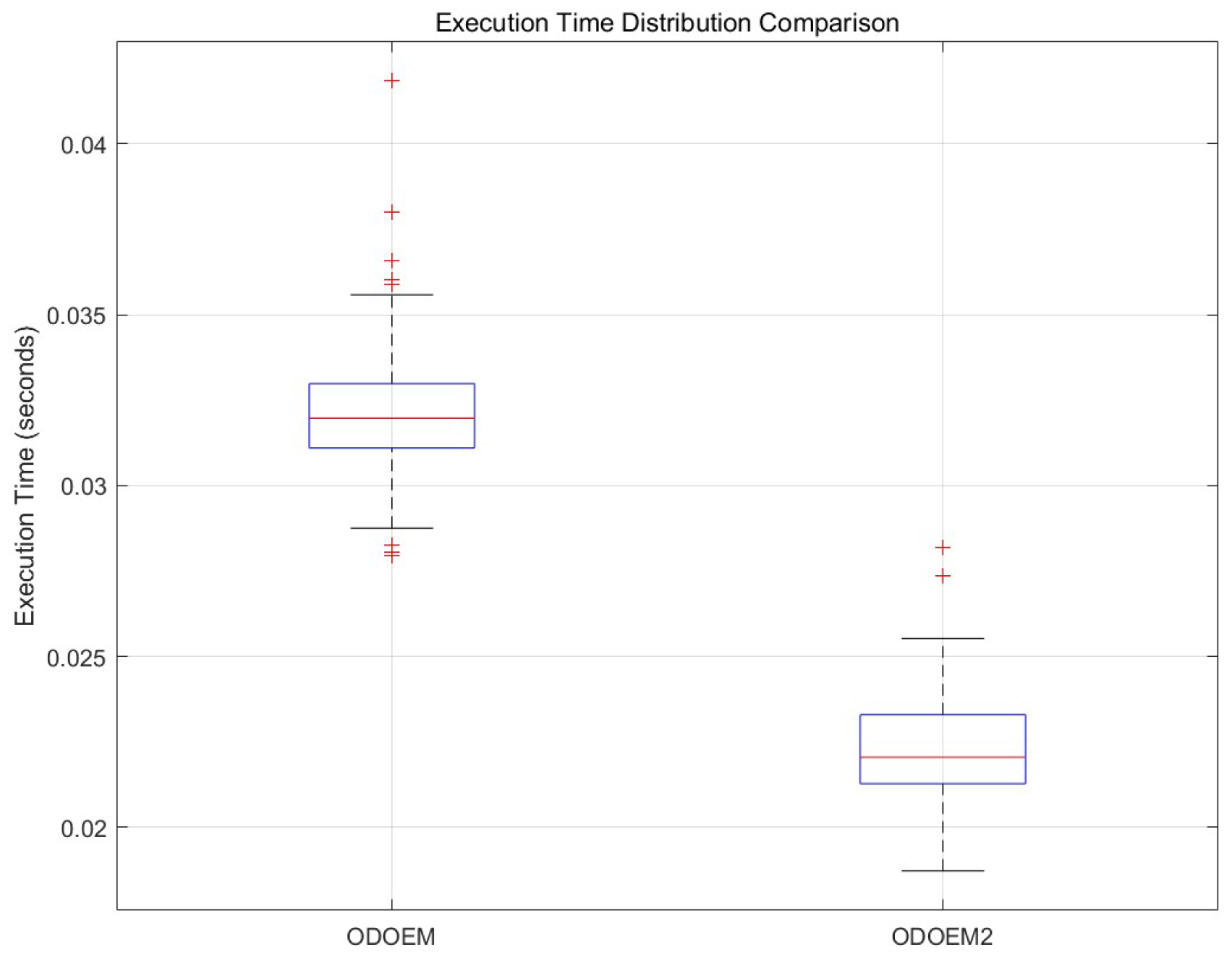
Finally, we compare the execution times of ODOEM and ODOEM2, both of which were implemented in Matlab R2023b. Figure 5 shows the distribution of execution times and the total execution time for each iteration. On average, Algorithm 2 runs 30.60% faster than Algorithm 1 (ODOEM: Mean = 0.0613 s per iteration, ODOEM2: Mean = 0.0425 s per iteration). Despite this difference, both algorithms are relatively fast.

5. Conclusions

In this paper, we reviewed the existing theoretical framework for D-optimal and G-optimal under the LapRLS model experimental designs on Riemannian manifolds. Building on this foundation, we extended the theory by investigating A-optimal experimental designs under the LapRLS model on manifolds. This extension led to the derivation of a new equivalence theorem specifically for A-optimality under the LapRLS model. Furthermore, we proposed a novel sequential algorithm tailored to efficiently find A-optimal experimental designs when only a finite set of candidate data points is available. We then compared our algorithms with the D-optimal design algorithm from Li and Del Castillo [14], and conducted numerical studies on synthetic and real-world datasets. The experimental results on synthetic and real datasets demonstrate the effectiveness of our proposed manifold-based A-optimal design algorithms. In particular, the results on real-world datasets in Section 4.2 show that while the two algorithms perform similarly, our method (Algorithm 2) achieves a slightly more uniform selection of image angles, marginally better prediction performance, and slightly faster runtime compared to Algorithm 1. These findings highlight the potential of A-optimal designs under the LapRLS model for improving experimental outcomes on Riemannian manifolds.

6. Discussion

Future research could focus on exploring optimal designs under other general optimality criteria, such as ${\varphi }_p$-optimality (see e.g., Chapter 6 of Pukelsheim [4]). Another direction for future work is to extend the results for the LapRLS regularization model to a broader range of models, including those with a more general loss function V in Equation (2), and models that are nonlinear in their parameters $\mathsf{\beta }$. This could offer deeper insights and more flexibility in addressing complex experimental design problems, especially in high-dimensional and nonlinear settings.

References

1. Kiefer, J.; Wolfowitz, J. The Equivalence of Two Extremum Problems. Can. J. Math. 1960, 12, 363–366. [Google Scholar] [CrossRef]
2. Fedorov, V.V. Design of Experiments for Linear Optimality Criteria. Theory Probab. Its Appl. 1971, 16, 189–195. [Google Scholar] [CrossRef]
3. Silvey, S.D. Optimal Design; Chapman and Hall: London, UK, 1980. [Google Scholar]
4. Pukelsheim, F. Optimal Design of Experiments; Society for Industrial and Applied Mathematics: Philadelphia, PA, USA, 2006. [Google Scholar]
5. Roweis, S.T.; Saul, L.K. Nonlinear Dimensionality Reduction by Locally Linear Embedding. Science 2000, 290, 2323–2326. [Google Scholar] [CrossRef] [PubMed]
6. Tenenbaum, J.B.; de Silva, V.; Langford, J.C. A Global Geometric Framework for Nonlinear Dimensionality Reduction. Science 2000, 290, 2319–2323. [Google Scholar] [CrossRef] [PubMed]
7. Donoho, D.; Grimes, C. Hessian Eigenmaps: Locally Linear Embedding Techniques for High Dimensional Data. Proc. Natl. Acad. Sci. USA 2003, 100, 5591–5596. [Google Scholar] [CrossRef] [PubMed]
8. Coifman, R.; Lafon, S.; Lee, A.; Maggioni, M.; Nadler, B.; Warner, F.; Zuker, S. Geometric Diffusions as a Tool for Harmonic Analysis and Structure Definition of Data: Diffusion Maps. Proc. Natl. Acad. Sci. USA 2005, 102, 7426–7431. [Google Scholar] [CrossRef] [PubMed]
9. Belkin, M.; Niyogi, P.; Sindhwani, V. Manifold Regularization: A Geometric Framework for Learning from Labeled and Unlabeled Examples. J. Mach. Learn. Res. 2006, 7, 2399–2434. [Google Scholar]
10. Meilă, M.; Zhang, H. Manifold Learning: What, How, and Why. Annu. Rev. Stat. Its Appl. 2024, 11, 393–417. [Google Scholar] [CrossRef]
11. He, X. Laplacian Regularized d-optimal Design for Active Learning and its Application to Image Retrieval. IEEE Trans. Image Process. 2010, 19, 254–263. [Google Scholar] [PubMed]
12. Chen, C.; Chen, Z.; Bu, J.; Wang, C.; Zhang, L.; Zhang, C. G-optimal Design with Laplacian Regularization. In Proceedings of the Twenty-Fourth AAAI Conference on Artificial Intelligence, Atlanta, GA, USA, 11–15 July 2010; Volume 1, pp. 413–418. [Google Scholar]
13. Alaeddini, A.; Craft, E.; Meka, R.; Martinez, S. Sequential Laplacian Regularized V-optimal Design of Experiments for Response Surface Modeling of Expensive Tests: An Application in Wind Tunnel Testing. IISE Trans. 2019, 51, 559–576. [Google Scholar] [CrossRef]
14. Li, H.; Del Castillo, E. Optimal Design of Experiments on Riemannian Manifolds. J. Am. Stat. Assoc. 2024, 119, 875–886. [Google Scholar] [CrossRef]
15. Jones, B.; Allen-Moyer, K.; Goos, P. A-Optimal versus D-Optimal Design of Screening Experiments. J. Qual. Technol. 2020, 53, 369–382. [Google Scholar] [CrossRef]
16. Stallrich, J.; Allen-Moyer, K.; Jones, B. D- and A-Optimal Screening Designs. Technometrics 2023, 65, 492–501. [Google Scholar] [CrossRef]
17. Domagni, F.K.; Hedayat, A.S.; Sinha, B.K. D-optimal saturated designs for main effects and interactions in 2k-factorial experiments. Stat. Theory Relat. Fields 2024, 8, 186–194. [Google Scholar] [CrossRef]
18. Belkin, M. Problems of Learning on Manifolds. Ph.D. Thesis, The University of Chicago, Chicago, IL, USA, 2003. [Google Scholar]
19. Schölkopf, B.; Smola, A.J. Learning with Kernels: Support Vector Machines, Regularization, Optimization, and Beyond; MIT Press: Cambridge, MA, USA, 2001. [Google Scholar]
20. Jayasumana, S.; Hartley, R.; Salzmann, M.; Li, H.; Harandi, M. Kernel Methods on Riemannian Manifolds with Gaussian RBF Kernels. IEEE Trans. Pattern Anal. Mach. Intell. 2015, 37, 2464–2477. [Google Scholar] [CrossRef] [PubMed]
21. Zhou, Z.-H. Machine Learning; Springer: Berlin/Heidelberg, Germany, 2021. [Google Scholar]
22. Singh, V.P.; Bokam, J.K.; Singh, S.P. Best-case, worst-case and mean integral-square-errors for reduction of continuous interval systems. Int. J. Artif. Intell. Pattern Recognit. 2020, 17, 17–28. [Google Scholar] [CrossRef]
Figure 1. Comparison of ODOEM and ODOEM2 designs on the Möbius strip and the saddle surface: (a,d): The colors represent the true response values defined on the Möbius strip and the saddle surface. (b,e): A hundred labeled instances (red numbers) and fitted response values (surface colors) by the ODOEM algorithm based on D-optimality under the LapRLS model (Algorithm 1). (c,f): A hundred labeled instances (red numbers) and fitted response values (surface colors) by the ODOEM2 algorithm based on A-optimality under the LapRLS model (Algorithm 2).
Axioms 14 00436 g001
Figure 2. First four images selected by ODOEM. The true angle is labeled on top of each image. (Left) ‘Lucky Cat’ data, (Right) ‘Car’ data.
Axioms 14 00436 g002
Figure 3. First four images selected by ODOEM2. The true angle is labeled on top of each image. (Left) ‘Lucky Cat’ data, (Right) ‘Car’ data.
Axioms 14 00436 g003
Figure 4. Comparisons of MSEs between Algorithms 1 (ODOEM) and 2 (ODOEM2). The horizontal axis represents the proportion of images labeled for each object. (Left) ‘Lucky Cat’ data, (Right) ‘Car’ data.
Axioms 14 00436 g004
Figure 5. Boxplots of execution time of each iteration of Algorithms 1 and 2.
Axioms 14 00436 g005
Disclaimer/Publisher’s Note: The statements, opinions and data contained in all publications are solely those of the individual author(s) and contributor(s) and not of MDPI and/or the editor(s). MDPI and/or the editor(s) disclaim responsibility for any injury to people or property resulting from any ideas, methods, instructions or products referred to in the content.