Exponential Squared Loss-Based Robust Variable Selection with Prior Information in Linear Regression Models

Abstract

This paper proposes a robust variable selection method that incorporates prior information through linear constraints. For more than a decade, penalized likelihood frameworks have been the predominant approach for variable selection, where appropriate loss and penalty functions are selected to formulate unconstrained optimization problems. However, in many specific applications, some prior information can be obtained. In this paper, we reformulate variable selection by incorporating prior knowledge as linear constraints. In addition, the loss function adopted in this paper is a robust exponential squared loss function, which ensures that the estimation of model parameter coefficient will not have a great impact when there are a few outliers in the dataset. This paper uses the designed solution algorithm to calculate the estimated values of coefficients and some other parameters, and finally conducts numerical simulations and a real-data experiment. Experimental results demonstrate that our model significantly improves estimation robustness compared to existing methods, even in outlier-contaminated scenarios.

1. Introduction

The selection of vital explanatory variables is one of the most important parts of statistics. For this reason, significant progress has been made in the penalty regression method, which performs parameter estimation and variable selection simultaneously. The Lasso method [1] and its derivatives, such as fused Lasso [2], adaptive Lasso [3], elastic network [4], etc., can be used to select variables and estimate coefficients of the model simultaneously, which is favored by many researchers. At the same time, due to its simplicity of solution, it also plays an important role in practical applications. The $L_0$ norm can also be used as a penalty term in the process of variable selection, but because its non-convexity solution is difficult to obtain, various algorithms are proposed and applied, for example, the Smoothed L0 (SL0) algorithm [5]. Tibshirani et al. [6] proposed the method of generalized Lasso. By designing the selection matrix, the generalized Lasso could be transformed into Lasso and adaptive Lasso. Moreover, the proof of its properties and the design of solving algorithm are given. However, both of the methods mentioned above are based on the least squares method. As we know, the least squares method does not have good robustness. In statistics, outliers refer to measured values that deviate from the mean by more than twice the standard deviation. When there are abnormal observations in a sample, the final estimations of coefficients in the model obtained using the least squares method are often greatly deviated. In a regression setting, the robustness of the estimator is closely related to the choice of loss function. Therefore, we consider choosing one robust loss to replace the least squares. Penalty robust regression, combining different loss functions and different penalty functions, has attracted significant attention and seen considerable development, for example, penalty regression based on Huber loss [7], Minimum Absolute Deviation (LAD)-Lasso [8], and penalty quantile regression [9]. Although these existing penalty regressions can yield robust parameter estimators, their robustness (such as breakdown point and impact function) has not been well characterized. To this end, a suitable variable selection process based on exponential squared loss is presented [10] and has proven to satisfy the $\sqrt{n}-$consistent and oracle properties. It also has better robustness and numerical performance than the penalty regression method mentioned above. Therefore, in this paper, the least squares component of the generalized Lasso is replaced by the exponential squared loss when constructing the objective model based on the method of a penalized likelihood framework [11], and the objective function of the model used in the later part is obtained.

In practical applications, there are many cases where we can obtain some information about the real model in advance, which is called prior information. The traditional way of using prior knowledge is via the Bayes method. We can also take advantage of prior information by setting constraints on parameters. For example, in the studies by Fan, Zhang, and Yu [12], the sum of all portfolio ratios is 1, which is a linear equation constraint. In this case, the problem of choosing the portfolio with the maximum return is transformed into a linear regression problem with a lasso penalty term and linear constraint. The shape of the non-parametric regression has some conditional restrictions [13], which requires adding linear inequality constraints to the coefficients to solve the regression problem. To solve the problems in the above application scenarios, corresponding models are respectively established. In addition, variable selection methods based on least squares [14] and robust quantile loss [15] under linear constraints are respectively established. Their studies also provide solution algorithms for the corresponding models and numerical simulation studies. However, these authors neither conducted simulations under outliers nor specifically described the robustness of their models. Moreover, variable selection methods based on quantile loss may experience reduced efficiency when normally distributed data are involved [16]. In this paper, for the convenience of studying the problem, we integrate the prior information into the variable selection model in the form of linear constraints, so as to build an optimization model under linear constraints. It is advisable to incorporate prior information into the objective model through linear constraints.

Based on the discussion above, we use the exponential squared loss function and generalized Lasso penalty to construct the objective model, and then incorporate it into the linear constraint conditions of prior information to build the following equation:

$$\underset{\beta }{min}\sum _{i=1}^n\{1-exp\{-{\displaystyle \frac{{(Y_i-X_i^T\beta )}^2}{\gamma }}\}\}+\lambda {\parallel D\beta \parallel }_1,$$

(1)

$$\mathrm{s}.\mathrm{t}.C\beta \ge d,$$

(2)

$$E\beta =f,$$

(3)

where $Y\in {\mathbb{R}}^n$ is the response variable, $X\in {\mathbb{R}}^{n\times p}$ is the design matrix, and $\beta \in {\mathbb{R}}^p$ is the parameter vector. Penalty matrix $D\in {\mathbb{R}}^{m\times p}$ is the matrix which is be chosen by real application. The choice of the punishment matrix D can vary, such as different forms of Lasso punishment, including Lasso, adaptive lasso, or fused lasso. $C\in {\mathbb{R}}^{q\times p}$, $d\in {\mathbb{R}}^q$, $E\in {\mathbb{R}}^{s\times p}$, and $f\in {\mathbb{R}}^s$ can be determined based on prior information. $\lambda$ and $\gamma$ are tuning parameters. ${\parallel ·\parallel }_1$ means ${\ell }_1$-norm of one vector.

In fact, the above model is an optimization problem of non-convex function under linear constraints, and it is often difficult to solve such a problem directly. Therefore, we aim to transform the model into a more tractable form before attempting to solve it. X. Wang et al. [10] showed that the exponential squared loss can be approximated via Taylor expansion, transformed into a quadratic model, and then solved by the Batch Size Gradient Descent (BSGD) method. Based on this, we first transform the model into a quadratic programming problem with linear constraints, then solve its dual model, and finally solve the dual problem using the coordinate descent method. Solving the dual problem is preferred because coordinate descent is significantly more efficient when applied to the dual problem than to the original quadratic programming problem [14]. The main contributions of this paper lie in the following aspects:

(i)

In terms of computing, an effective algorithm is designed in this paper. The original non-convex model is transformed, then parameters ($\gamma$ and $\lambda$) in the model are selected using established criteria, and finally, coefficients are estimated by the designed algorithm.

(ii)

In terms of theory, based on the research work of some scholars, a formula for calculating model degrees of freedom is developed to measure model complexity.

(iii)

In terms of robustness, three sets of simulated data with different outliers are designed in this paper. The results obtained by the model on these three sets of data are in line with expectations, which indicates that the model has the ability to resist noise points or outliers.

This paper is organized as follows. In Section 2, we elaborate on the construction method of our model, derive its dual form, and calculate the degrees of freedom. In Section 3, we present the parameter selection method and establish the solution algorithm of the model. In Section 4, we design two sets of experiments: numerical simulation and real-data experimentation. Finally, we summarize and discuss this paper.

2. Methodology

This section covers several topics related to the proposed method. Firstly, we discuss some basic contents of exponential squared loss function. Then, a robust variable selection method with linear constraints is constructed on the basis of this loss function. Next, this problem is transformed into a quadratic programming formulation with linear constraints. Afterwards, the dual form of the transformed quadratic programming problem is derived, along with the Karush–Kuhn–Tucker (KKT) conditions of its dual solution, which is the optimality criteria for constrained nonlinear programming problems. Finally, the degrees of freedom related to model complexity are discussed.

2.1. Exponential Squared Loss Function

In the design of the variable selection method, the choice of loss function often determines the robustness. The exponential squared loss function enhances robustness against outliers by imposing an exponential decay on the gradient magnitude for large residuals. Unlike the squared error loss, whose gradient grows linearly with residuals, the exponential squared loss suppresses the influence of large errors through its multiplicative exponential term. This bounded gradient ensures that outliers contribute minimally to parameter updates, while smaller residuals retain near-quadratic behavior for efficient learning. Exponential squared loss has been shown to perform well as a loss function in AdaBoost for classification problems [17]. Specifically, AdaBoost (Adaptive Boosting), a well-known ensemble learning algorithm for classification that iteratively adjusts sample weights and combines weak classifiers through weighted majority voting, demonstrated enhanced robustness against label noise when employing this loss function. In the regression field, X. Wang et al. [10] used exponential squared loss to design a noise-resistant variable selection method, which also performed well. In energy management systems, the exponential squared loss function can be used to make robust estimates of signal states with errors [18]. In this paper, we also use this loss function to construct a robust model with linear constraints.

The exponential squared loss function has the following form:

$${\varphi }_{\gamma }\left(t\right)=1-exp(-t^2/\gamma ).$$

(4)

In (4), $t=Y-x^T\beta$, which represents one regression residual. $\gamma$ is a tuning parameter, whose numerical value determines the robustness in the estimation of coefficients. Under large $\gamma$ conditions (usually greater than 10), the ${\varphi }_{\gamma }\left(t\right)$ is approximately equal to $t^2/\gamma$, leading the estimators to closely resemble least squares methods in limiting cases. When $\gamma$ is small, observations with large absolute values of t will lead to large losses of ${\varphi }_{\gamma }\left(t\right)$, which diminishes their impact to $\beta$ parameter estimation. 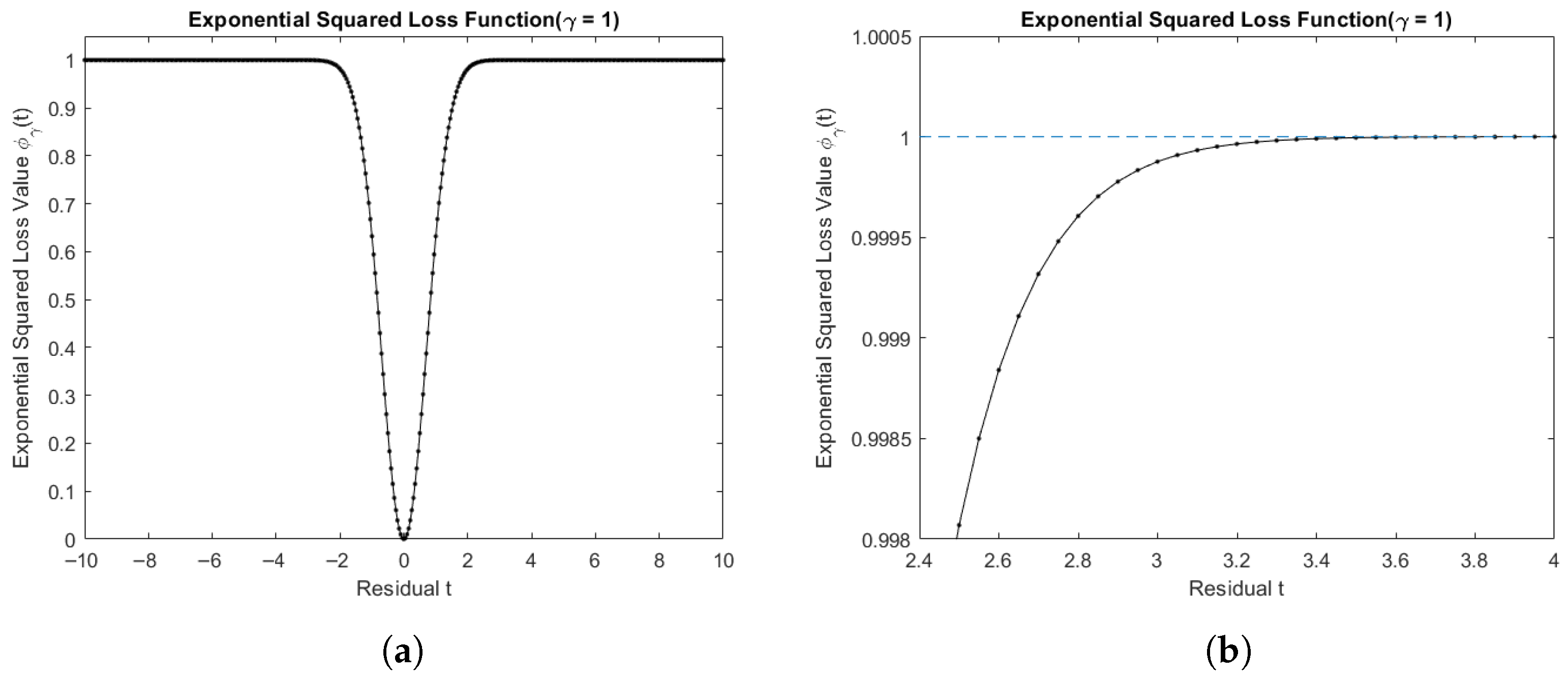Therefore, selecting a smaller $\gamma$ value limits the impact of an outlier on the estimators; this comes at the cost of decreased estimator responsiveness to data variations. We use the following two images to intuitively explain why the exponential squared loss function is of certain robustness.

Firstly, we consider $\gamma$ as a small fixed value. When there are noise points or abnormal data in the samples, the absolute value of residual t tends to be larger. From Figure 1a,b, we can see that the value of the exponential squared loss function gradually approaches 1 as the absolute value of residual t increases, which would have a small impact on the estimation of $\beta$. In contrast, as the absolute value of the residual t increases, the least squares loss function will result in a larger loss value, which leads to an inaccurate estimation of $\beta$.

When the value of $\gamma$ is significantly high, we can consider $-t^2/\gamma \approx 0$. According to the theorem of infinitesimal substitution of equal values, we can determine that ${\varphi }_{\gamma }\left(t\right)\approx t^2/\gamma$. This approximation implies that the exponential squared is analogous to the least squares loss.

In conclusion, the selection of the parameter $\gamma$ in the exponential squared loss function should be guided by the statistical properties of the data and the desired robustness–efficiency trade-off.

2.2. Penalized Exponential Squared Loss with Linear Constraints

The idea of model construction is as follows: Firstly, we design a general unconstrained variable selection method based on exponential squared loss and generalized Lasso penalty. Then, prior information is incorporated into the variable selection method as constraints. Finally, variable selection is reformulated as a constrained optimization problem. Notably, we mainly consider the case where prior information exists as linear constraints.

The model we built is as follows:

$$\begin{array}{cc}\hfill \underset{\beta }{min}& \sum _{i=1}^n\{1-exp\{-{\displaystyle \frac{{(Y_i-x_i^T\beta )}^2}{\gamma }}\}\}+\lambda {\parallel D\beta \parallel }_1,\hfill \end{array}$$

(5)

$$\begin{array}{cc}\hfill \mathrm{s}.\mathrm{t}.& C\beta \ge d,\hfill \end{array}$$

(6)

$$\begin{array}{cc}& E\beta =f,\hfill \end{array}$$

(7)

where $Y\in {\mathbb{R}}^n$, $X\in {\mathbb{R}}^{n\times p}$, $\beta \in {\mathbb{R}}^p$. $D\in {\mathbb{R}}^{m\times p}$ is a matrix that is chosen based on the application. $C\in {\mathbb{R}}^{q\times p}$, $d\in {\mathbb{R}}^q$, $E\in {\mathbb{R}}^{s\times p}$, and $f\in {\mathbb{R}}^s$ can be determined based on prior information. ${\parallel ·\parallel }_1$ represents the ${\ell }_1$-norm of a vector. We know that the existence of a constant term has no effect on the solution of an optimization model. Therefore, we remove the constant term in Equation (5), and the model is changed into the following form:

$$\begin{array}{cc}\hfill \underset{\beta }{max}& {\ell }_n\left(\beta \right)=\sum _{i=1}^{n}exp\{-{\displaystyle \frac{{(Y_i-x_i^T\beta )}^2}{\gamma }}\}-\lambda {\parallel D\beta \parallel }_1,\hfill \end{array}$$

(8)

$$\begin{array}{cc}\hfill \mathrm{s}.\mathrm{t}.& C\beta \ge d\hfill \end{array}$$

(9)

$$\begin{array}{cc}& E\beta =f.\hfill \end{array}$$

(10)

Equation (8) contains the non-convex term $exp-{(Y_i-x_i^T\beta )}^2/\gamma$. As a result, the computational complexity of finding a numerical solution is high, making the programming process challenging. For this reason, we consider applying some transformation to Equation (8) to turn it into a form that can be easily processed. The basic idea behind this transformation is Taylor expansion. This strategy has also been employed in prior research [7,10,18]. Specifically, we use the Taylor formula to expand the exponential squared function in Equation (8). By discarding terms above the second order, we convert the exponential squared function into a quadratic form.

Let

$${\ell }^{*}\left(\beta \right)=\sum _{i=1}^{n}exp\{-{(Y_i-x_i^T\beta )}^2/\gamma \}.$$

(11)

Assuming that ${\beta }^0$ is the initial estimate of the coefficients for the explanatory variables, we can obtain this value using various methods, such as via an MM-estimator (multiple M-estimator, a robust regression method involving two M-estimation steps), a least squares estimator, and so on. It is obtained by solving the objective function with only the loss function (${\ell }^{*}\left(\beta \right)$) and no penalty term, so ${\nabla }^1{\ell }^{*}\left({\beta }^0\right)=0$ is valid. We can use Taylor’s formula to expand (11) at ${\beta }^0$ to get

$${\ell }^{*}\left(\beta \right)\approx {\ell }^{*}\left({\beta }^0\right)+{\displaystyle \frac{1}{2}}{(\beta -{\beta }^0)}^T{\nabla }^2{\ell }^{*}\left({\beta }^0\right)(\beta -{\beta }^0)$$

(12)

Substituting Equation (12) into (8), the model can be transformed into the following form:

$$\begin{array}{cc}\hfill \underset{\beta }{max}& {\ell }_n\left(\beta \right)={\ell }^{*}\left({\beta }^0\right)+{\displaystyle \frac{1}{2}}{(\beta -{\beta }^0)}^T{\nabla }^2{\ell }^{*}\left({\beta }^0\right)(\beta -{\beta }^0)-\lambda {\parallel D\beta \parallel }_1,\hfill \end{array}$$

(13)

$$\begin{array}{cc}\hfill \mathrm{s}.\mathrm{t}.& C\beta \ge d\hfill \end{array}$$

(14)

$$\begin{array}{cc}& E\beta =f,\hfill \end{array}$$

(15)

where ${\nabla }^2{\ell }^{*}\left({\beta }^0\right)$ is the Hessian matrix of ${\ell }^{*}\left(\beta \right)$ at ${\beta }^0$. Formulas (13) to (15) are quadratic programming problems with linear constraints, which are easier to solve than the original model. Next, we consider removing the constant term ${\ell }^{*}\left({\beta }^0\right)$ from Equation (13), which is independent of optimization. Simultaneously, we also consider the processing of the Hessian matrix, so as to further simplify the model.

The Hessian matrix is represented as $Q\left(\beta \right)$. According to the previous statement, the following is true:

$$Q\left({\beta }^0\right)={\nabla }^2{\ell }^{*}\left({\beta }^0\right).$$

$Q\left(\beta \right)$ can be calculated using the following formula:

$$Q=-H^{T}W\left(x\right)[I-diag({\displaystyle \frac{{(Y-X^T\beta )}^2}{\gamma /2}})]H$$

$H\left(x\right)$ is a Jacobian matrix. $W\left(x\right)$ is a diagonal matrix, $W_{ii}=2w_i\left(x\right)/\gamma$, where $w_i\left(x\right)=exp(-{(Y_i-x_i^T\beta )}^2/\gamma )$. Existing research [18] shows that for the model defined by Equations (13)–(15) to attain its maximum, matrix Q must be negative definite. Let

$$\Phi =W\left[I-diag(2{(Y-X^T\beta )}^2/\gamma )\right].$$

Therefore, $Q=-H^T\Phi H$. At the same time, $\Phi$ is a diagonal matrix. Based on the algebraic theory, if all ${\Phi }_{ii}>0$, then $\Phi$ is a positive definite matrix, which makes Q negative. However, when there are outliers or contaminated data, some residuals will be too large and the corresponding diagonal elements will be negative. Therefore, we need to relax the condition of $\Phi$ as follows:

$${\Phi }_{ii}>ϵ,\forall i.$$

(16)

$ϵ$ in (16) is a small negative number, such as −0.01, which is selected according to the specific situation of the problem. If (16) is true in the study, we also believe that the second-order condition of the optimization problem is satisfied.

We now rearrange Equation (13): since it serves as the optimization objective function, its constant term does not affect the solution. Therefore, we remove the constant term from (13). Then, we rewrite (13) as follows:

$${\ell }_n\left(\beta \right)={\displaystyle \frac{1}{2}}{(\beta -{\beta }^0)}^T{\nabla }^2{\ell }^{*}\left({\beta }^0\right)(\beta -{\beta }^0)-\lambda {\parallel D\beta \parallel }_1.$$

(17)

Substituting the above discussion of the Hessian matrix into (17), we obtain

$${\ell }_n\left(\beta \right)={\displaystyle \frac{1}{2}}{(\beta -{\beta }^0)}^{T}Q\left({\beta }_0\right)(\beta -{\beta }^0)-\lambda {\parallel D\beta \parallel }_1.$$

Finally, we get

$$\begin{array}{cc}\hfill \mathrm{s}.\mathrm{t}.& C\beta \ge d,\hfill \\ & E\beta =f,\hfill \end{array}$$

where

$$S=H^{T}W\left(x\right)[I-diag({\displaystyle \frac{{(Y-X^T{\beta }_0)}^2}{\gamma /2}})]H.$$

(18)

$$r=S{\beta }^0.$$

(19)

The above is equivalent to

$$\begin{array}{cc}\hfill \underset{\beta }{min}& {\ell }_n\left(\beta \right)={\displaystyle \frac{1}{2}}{\beta }^{T}S\beta -r^T\beta +\lambda {\parallel D\beta \parallel }_1,\hfill \end{array}$$

(20)

$$\begin{array}{cc}\hfill \mathrm{s}.\mathrm{t}.& C\beta \ge d,\hfill \end{array}$$

(21)

$$\begin{array}{cc}& E\beta =f.\hfill \end{array}$$

(22)

In this way, (20)–(22) is the model we will solve later in the paper, which is much easier to handle than the previous model (13)–(15).

2.3. The Dual Problem and KKT Conditions

We adopted a methodology similar to Hu et al. [14] for processing model (20)–(22). However, there is a difference between (20) and their model, which lies in the values of the variables S and r. In their study, S and r are

$$S=X^{T}X$$

$$r=X^{T}y,$$

which are obviously different from (18) and (19).

The aim of our research is to analyze the model (20)–(22). First, we derive the primal problem’s dual form. Then, we analyze the dual solution’s properties through its KKT conditions. Next, we present a proposition that establishes the relationship between the dual problem and the primal model. Finally, Section 3 develops a coordinate descent algorithm for the dual model.

We introduce a new variable $z=D\beta$ into (20). The model can be transformed into the following form:

$$\begin{array}{cc}\hfill \underset{\beta }{min}& {\ell }_n\left(\beta \right)={\displaystyle \frac{1}{2}}{\beta }^{T}S\beta -r^T\beta +\lambda {\parallel z\parallel }_1,\hfill \end{array}$$

(23)

$$\begin{array}{cc}\hfill \mathrm{s}.\mathrm{t}.& D\beta =z,\hfill \end{array}$$

(24)

$$\begin{array}{cc}& C\beta \ge d,\hfill \end{array}$$

(25)

$$\begin{array}{cc}& E\beta =f.\hfill \end{array}$$

(26)

The Lagrangian equation of the above model is as follows:

$$L(\beta ,z,u,\xi ,\eta )={\displaystyle \frac{1}{2}}{\beta }^{T}S\beta -r^T{\parallel z\parallel }_1+u^T(D\beta -z)-{\xi }^T(C\beta -d)-{\eta }^T(E\beta -f).$$

where $u={(u_1,u_2,\dots ,u_m)}^T\in {\mathbb{R}}^m$, $\xi ={({\xi }_1,{\xi }_2,\dots ,{\xi }_q)}^T\in {\mathbb{R}}^q$, and $\eta ={({\eta }_1,{\eta }_2,\dots ,{\eta }_s)}^T\in {\mathbb{R}}^s$ are Lagrange multipliers. Each of the ${\xi }_i$ is non-negative for $i=1,\dots ,q$. Therefore, the resulting Lagrangian dual function is as follows:

$$Q^{*}(u,\xi ,\eta )=\underset{\beta ,z}{min}L(\beta ,z,u,\xi ,\eta ).$$

Boyd and Vandenberghe [19] have discussed the duality problem under convex optimization in detail. Since matrix S is positive definite, Equation (23) is convex. Moreover, all constraints are linear, so the model including (23)–(26) is a convex optimization problem. We know that the primal model minimization is equivalent to the dual problem maximization.

We can divide L into the sum of two functions. One is related to $\beta$ and another is only concerned with z:

$$L(\beta ,z,u,\xi ,\eta )=L_1(\beta ,u,\xi ,\eta )+L_2(z,u).$$

$$L_1(\beta ,u,\xi ,\eta )={\displaystyle \frac{1}{2}}{\beta }^{T}S\beta -r^T\beta +u^{T}D\beta -{\xi }^T(C\beta -d)-{\eta }^T(E\beta -f).$$

$$L_2(z,u)=\lambda {\parallel z\parallel }_1-u^{T}z.$$

Minimizing L is equivalent to minimizing both $L_1$ and $L_2$ simultaneously. When $L_1$ takes the minimum value, the corresponding value of parameter $\beta$ is

$$\beta =S^{-1}(r-D^{T}u+C^T\xi +E^T\eta ).$$

The result of minimizing $L_2$ is

$$\underset{z}{min}{L}_2(z,u)=\left\{\begin{array}{ccc}0\hfill & & {\mathrm{if}\parallel u\parallel }_{\infty }\le \lambda \hfill \\ -\infty \hfill & & \mathrm{otherwise}\hfill \end{array}\right.$$

where ${\parallel u\parallel }_{\infty }={max}_k\left|u_k\right|$ is the ∞-norm of u. The dual model of the original problem obtained is

$$\begin{array}{cc}\hfill \underset{u,\xi ,\eta }{min}& P(u,\xi ,\eta ),\hfill \\ \hfill \mathrm{s}.\mathrm{t}.& {\parallel u\parallel }_{\infty }\le \lambda ,\hfill \\ & {\xi }_k\ge 0k=1,\dots ,q,\hfill \end{array}$$

where

$$P(u,\xi ,\eta )={\displaystyle \frac{1}{2}}{(r-D^{T}u+C^T\xi +E^T\eta )}^T{S}^{-1}(r-D^{T}u+C^T\xi +E^T\eta )-d^T\xi -f^T\eta .$$

We transform the original problem into its dual form because coordinate descent is more efficient on the dual than on the primal problem. The KKT conditions for the dual model are given below:

$$-D{S}^{-1}(r-D^{T}u+C^T\xi +E^T\eta )+v^{+}-v^{-}=0,$$

$$C{S}^{-1}(r-D^{T}u+C^T\xi +E^T\eta )-\tau =d,$$

$$E{S}^{-1}(r-D^{T}u+C^T\xi +E^T\eta )=f,$$

$$v_k^{+}(u_k-\lambda )=0,$$

$$v_k^{-}(u_k+\lambda )=0,$$

$${\tau }_k{\xi }_k=0,$$

where $v_k^{+}\ge 0$, $v_k^{-}\ge 0$ and ${\tau }_k\ge 0$. When ${\widehat{u}}_k=\pm \lambda$ or ${\widehat{\xi }}_k=0$ is known, the KKT conditions above can be simplified. Firstly, we need to define two boundary sets for the dual problem: $\mathcal{U}=\{i:|{\widehat{u}}_i|=\lambda \}$ and $\mathcal{C}=\{k:{\widehat{\xi }}_k=0\}$. Both sets are related to $\lambda$. By substituting Equation (7) into the KKT conditions above, we obtain

$$D_k\beta =s_k{a}_{k}k\in \mathcal{U},$$

$$D_k\beta =0k\notin \mathcal{U},$$

$$C_k\beta =d_k+{\tau }_{k}k\in \mathcal{C},$$

$$C_k\beta =d_{k}k\notin \mathcal{C},$$

$$E_k\beta =f_k\forall k.$$

In fact, the primal model also has two similar boundary sets, which have been discussed in some studies [14], so this paper will not go into detail.

Here, we provide a proposition that describes the uniqueness of the solution.

Proposition 1.

If S is positive definite, then $\widehat{\beta }$ and $\widehat{\mu }$ are unique, where $\widehat{\mu }=X\widehat{\beta }$.

The proof of Proposition 1 is as follows.

Considering the model including (20)–(22), the objective function (20)’s Hessian matrix is

$${\nabla }^2{\ell }_n\left(x\right)=S.$$

Since S is positive definite, we can determine that (20) is a strictly convex function.

Assuming that both ${\beta }^1$ and ${\beta }^2$ are the minimizers of the model including (20) and (21), where ${\beta }^1\ne {\beta }^2$, then we have

$$Q_{min}=Q\left({\beta }^1\right)=Q\left({\beta }^2\right)$$

At the same time, we know

$$C{\beta }^{\left(i\right)}>d,E{\beta }^{\left(i\right)}=f,i=1,2.$$

Let ${\beta }^{\prime }=(1-\alpha ){\beta }^1+\alpha {\beta }^2, 0<\alpha <1$; it is easy to know that ${\beta }^{\prime }$ satisfies all of the linear constraints. Therefore, we have

$$Q\left({\beta }^{\prime }\right)=Q((1-\alpha ){\beta }^1+\alpha {\beta }^2)\le (1-\alpha )Q\left({\beta }^1\right)+\alpha Q\left({\beta }^2\right)=Q_{min},$$

where the equality holds only when ${\beta }^1={\beta }^2$. This is inconsistent with the requirements of ${\beta }^1\ne {\beta }^2$. Therefore, $\widehat{\beta }$ is unique. In the meantime, since $\widehat{\mu }=S\widehat{\beta }$, we can determine that $\widehat{\mu }$ is also unique.

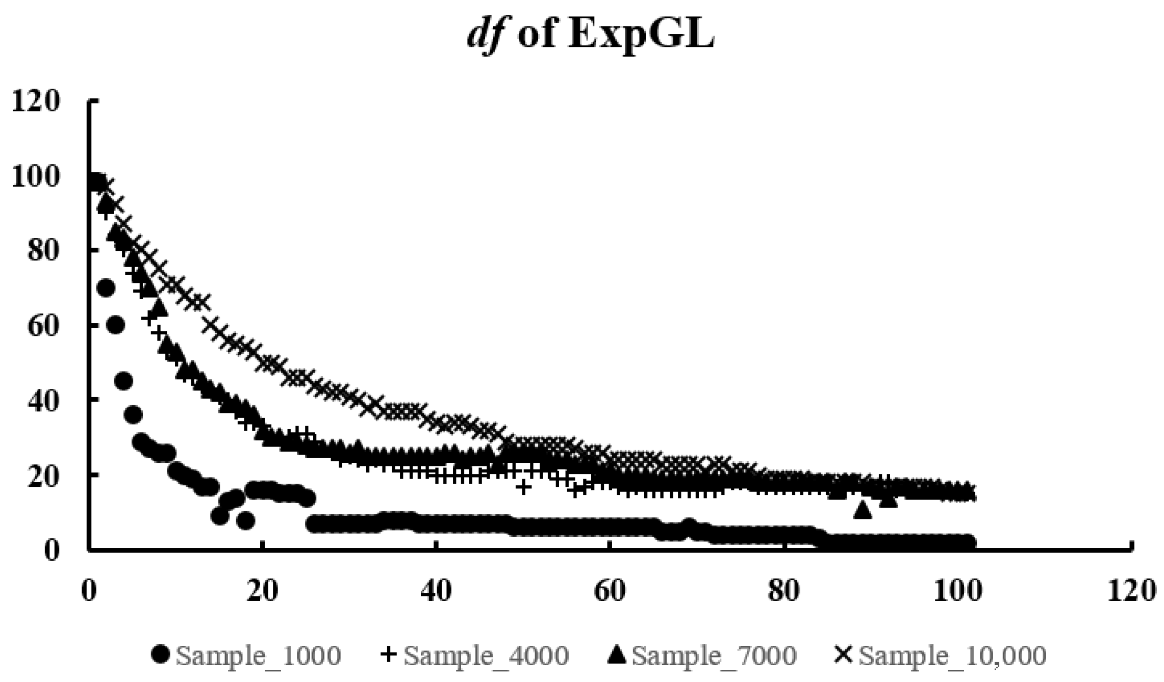
2.4. Degrees of Freedom

The degrees of freedom actually introduce a measure of the complexity of a model. We know that the same problem may admit multiple modeling approaches. It is not possible to directly compare the results of each model, because the number of parameters in each model is not the same. However, the results of different models can be compared at the same degrees of freedom, which can be used for model selection and assessment.

When studying the theory of unbiased risk estimation, Stein [20] proposed a method to calculate the degrees of freedom. Later, on the basis of Stein’s work, Efron [21] studied a new estimation method, which can be reduced to Stein’s estimate formula in some cases. We assume that $Y={(Y_1,\dots ,Y_n)}^T\sim N(\mu ,{\sigma }^{2}I)$, $Y_i,i=1,\dots ,n$ are independent of each other. Here, the superscript “T” denotes the transpose; the notation $N(\mu ,{\sigma }^{2}I)$ denotes that Y has a normal distribution with mean $\mu$ and variance ${\sigma }^{2}I$, where I is the identity matrix. Let $\widehat{Y}=g(X,Y)$, where g is a statistical model. The degree of freedom of the model can be calculated by the following formula:

$$df\left(g\right)=\sum _{i=1}^{n}Cov({\widehat{Y}}_i,Y_i)/{\sigma }^2.$$

The above formula can be interpreted as indicating that predictive performance improves with increasing model complexity. As a result, stronger correlation emerges between the observed samples and the predicted data. Ultimately, it leads to higher degrees of freedom. When Y is normally distributed, there is $Cov({\widehat{Y}}_i,Y_i)={\sigma }^{2}E(\partial {\widehat{Y}}_i/\partial Y_i)$. If $\widehat{Y}$ is a continuously differentiable function of Y, then we have

$$df\left(g\right)=\sum _{i=1}^{n}E\left({\displaystyle \frac{\partial {\widehat{Y}}_i}{\partial Y_i}}\right),$$

which is Stein’s estimate. In order to apply the above theory, we need to prove that $\widehat{Y}$ is a continuous and almost differentiable function of Y. In fact, according to Hu et al. [14], we can prove that given $\lambda$, $\beta$ is continuous and $\widehat{Y}$ satisfies a uniformly Lipschitz condition. We give three lemmas in the following text. Based on these and Hu et al. [14], we derive the formula for calculating degrees of freedom for the dual problem.

Lemma 1.

For any fixed λ, there is a set ${\mathcal{N}}_{\lambda }$, whose measure is zero. For $\forall Y\notin {\mathcal{N}}_{\lambda }$, there is always a neighbourhood where $\mathcal{U}$ and $\mathcal{C}$ are constant.

Lemma 2.

For any fixed λ, $\widehat{\beta }$ is a continuous function about Y.

Lemma 3.

For any fixed $\lambda \ge 0$ and $Y\notin {\mathcal{N}}_{\lambda }$, $\widehat{Y}=X\widehat{\beta }$ is uniformly Lipschitz.

Then, we can obtain the following theorem.

Theorem 1.

Assuming that Y is a random vector consisting of independent random variables, each has a normal distribution. For any matrices D, C, E and any scalar $\lambda \ge 0$, we can obtain the formula for the degrees of freedom. Here, $D_{-\mathcal{U}}$ denotes the matrix D with the rows or columns associated with u removed, and $C_{-\mathcal{C}}$ is defined analogously.

$$df(\widehat{Y})=\mathbb{E}\left[nullity\left(\begin{array}{c}{D}_{-\mathcal{U}}\\ -C_{-\mathcal{C}}\\ -E\end{array}\right)\right].$$

3. Choice of Tuning Parameter and Algorithm Designing

In this section, the coordinate descent method is used to solve the dual model. However, there are other parameters in the model besides $\beta$, such as $\gamma$ and $\lambda$. Therefore, we also need to introduce corresponding methods for the selection of $\gamma$ and $\lambda$.

3.1. Selection of $\gamma$

The selection of $\gamma$ determines the robustness of coefficient estimations, or in other words, the sensitivity to outliers. Following X. Wang et al. [10], we obtain a $\gamma$ selection method according to sample data, which can bypass prior identification and processing of outliers. In the meantime, the value of $\gamma$ obtained by this method is of high efficiency and robustness. This approach can be broken down into the following two steps:

1. Determining the set of outliers in the sample

Let $D_n=\{(x_1,Y_1),(x_2,Y_2),\dots ,(x_n,Y_n)\}$. First, we calculate $r_i\left(\widehat{\beta }\right)=Y_i-x_i^T\widehat{\beta }$. Next, we obtain $S_n=1.4826\times |r_i(\widehat{\beta })-media{n}_j(r_j(\widehat{\beta }))|$. Finally, we can determine the set of outliers as follows: $D_m=\{(x_i,y_i): |r_i\widehat{\beta }| \ge 2.5S_n\}$. Let $m=♯\{1\le i\le n:|r_i(\widehat{\beta })|\ge 2.5S_n\}$, $D_{n-m}=D_n/D_m$.

2. Updating $\mathbf{\gamma }$

$\gamma$ is essentially minimizing the $det(\widehat{V}\left(\gamma \right))$ on the set $G=\{\gamma :\varsigma (\gamma )\in (0,1]\}$, where

$$\varsigma \left(\gamma \right)={\displaystyle \frac{2m}{n}}+{\displaystyle \frac{2}{n}}\sum _{i=m+1}^n{\varphi }_{\gamma }\{r_i(\widehat{\beta })\}.$$

det() is the determinant and $\widehat{V\left(\gamma \right)}={\{{\widehat{I}}_1(\widehat{\beta })\}}^{-1}{\Sigma }_2{{\widehat{I}}_1(\widehat{\beta })}^{-1}$, where

$${\widehat{I}}_1({\widehat{\beta }}_n)={\displaystyle \frac{2}{\gamma }}\{{\displaystyle \frac{1}{2}}\sum _{i=1}^{n}exp(-r_i^2(\widehat{\beta }/\gamma ))\left({\displaystyle \frac{2r_i^2(\widehat{\beta })}{\gamma }}-1\right)\}\times \left({\displaystyle \frac{1}{n}}\sum _{i=1}^n{x}_i{x}_i^T\right)$$

$${\Sigma }_2=Cov\{exp\left(-r_1^2(\widehat{\beta })/\gamma \right){\displaystyle \frac{2r_1(\widehat{\beta })}{\gamma }}{x}_1,\dots ,exp\left(-r_n^2(\widehat{\beta })/\gamma \right){\displaystyle \frac{2r_n(\widehat{\beta })}{\gamma }}{x}_n\}.$$

In this way, we can obtain an estimate of $\gamma$.

3.2. Updating $\beta$

Hu et al. [14] proposed the coordinate descent method for the dual model of a quadratic programming problem under linear constraints. Taking their work into consideration, we first define a few new matrices as follows:

$$P_E=E^T{\left(E{S}^{-1}{E}^T\right)}^{-1}E{S}^{-1}.$$

$$\tilde{r}=(I-P_E)r+E^T{\left(E{S}^{-1}{E}^T\right)}^{-1}f.$$

$$\tilde{D}=D(I-P_E^T).$$

$$\tilde{C}=C(I-P_E^T).$$

$$\tilde{d}=d-C{S}^{-1}{E}^T{\left(ES{E}^T\right)}^{-1}f.$$

$$\tilde{g}=D{S}^{-1}{E}^T{\left(E{S}^{-1}{E}^T\right)}^{-1}f.$$

Before we give the coordinate descent algorithm for the dual problem

$$\begin{array}{cc}\hfill \underset{u,\xi ,\eta }{min}& P(u,\xi ,\eta ),\hfill \end{array}$$

(27)

$$\begin{array}{cc}\hfill \mathrm{s}.\mathrm{t}.& {\parallel u\parallel }_{\infty }\le \lambda ,\hfill \end{array}$$

(28)

$$\begin{array}{cc}& {\xi }_k\ge 0k=1,\dots ,q,\hfill \end{array}$$

(29)

the calculation formula of the primal solution can be given:

$$\beta =S^{-1}(\tilde{r}-{\tilde{D}}^{T}u+{\tilde{C}}^T\xi ).$$

The four steps of the coordinate descent method are given below:

1. The initial value of $\beta$ can be given by a robust estimate such as the MM estimator. At the same time, we set the initial values of u and $\xi$ as the zero vectors.

2. Update every component of u. We define the current kth component to be ${\tilde{u}}_k^{\left(0\right)}$ and the latest estimate of $\beta$ as ${\widehat{\beta }}^{\left(0\right)}$. First, calculate ${\widehat{u}}_k^{*}={\widehat{u}}_k^{\left(0\right)}+({\tilde{g}}_k+{\tilde{D}}_k^T\widehat{\beta })/({\tilde{D}}_k^T{S}^{-1}{\tilde{D}}_k)$. Then, update ${\widehat{u}}_k=sign\left({\widehat{u}}_k^{*}\right)[\lambda -(\lambda -|{\widehat{u}}_k^{*}{\left|\right)}_{+}]$. Finally, we can obtain $\widehat{\beta }={\widehat{\beta }}^0-S^{-1}{\tilde{D}}_k({\widehat{u}}_k-{\widehat{u}}_k^{\left(0\right)})$.

3. Update every component of $\xi$. We define the current kth component to be ${\tilde{\xi }}_k^{\left(0\right)}$ and the latest estimate of $\beta$ as ${\widehat{\beta }}^{\left(0\right)}$. First, calculate ${\widehat{\xi }}_k^{*}={\widehat{\xi }}_k^{\left(0\right)}+({\tilde{d}}_k-{\tilde{C}}_k^T\beta )/({\tilde{C}}_k^T{S}^{-1}{\tilde{C}}_k)$. Then, update $\widehat{\xi }={({\widehat{\xi }}_k^{*})}_{+}$. Finally, we can obtain $\widehat{\beta }={\widehat{\beta }}^{\left(0\right)}+S^{-1}{\tilde{C}}_k({\widehat{\xi }}_k-{\widehat{\xi }}_k^{\left(0\right)})$.

4. Calculate the value of P using Equation (27) to check for convergence. If the value of P in (27) obtained over two consecutive times satisfies the convergence condition, we stop the iteration and output the estimation of $\beta$. Otherwise, repeat 2–3 until convergence.

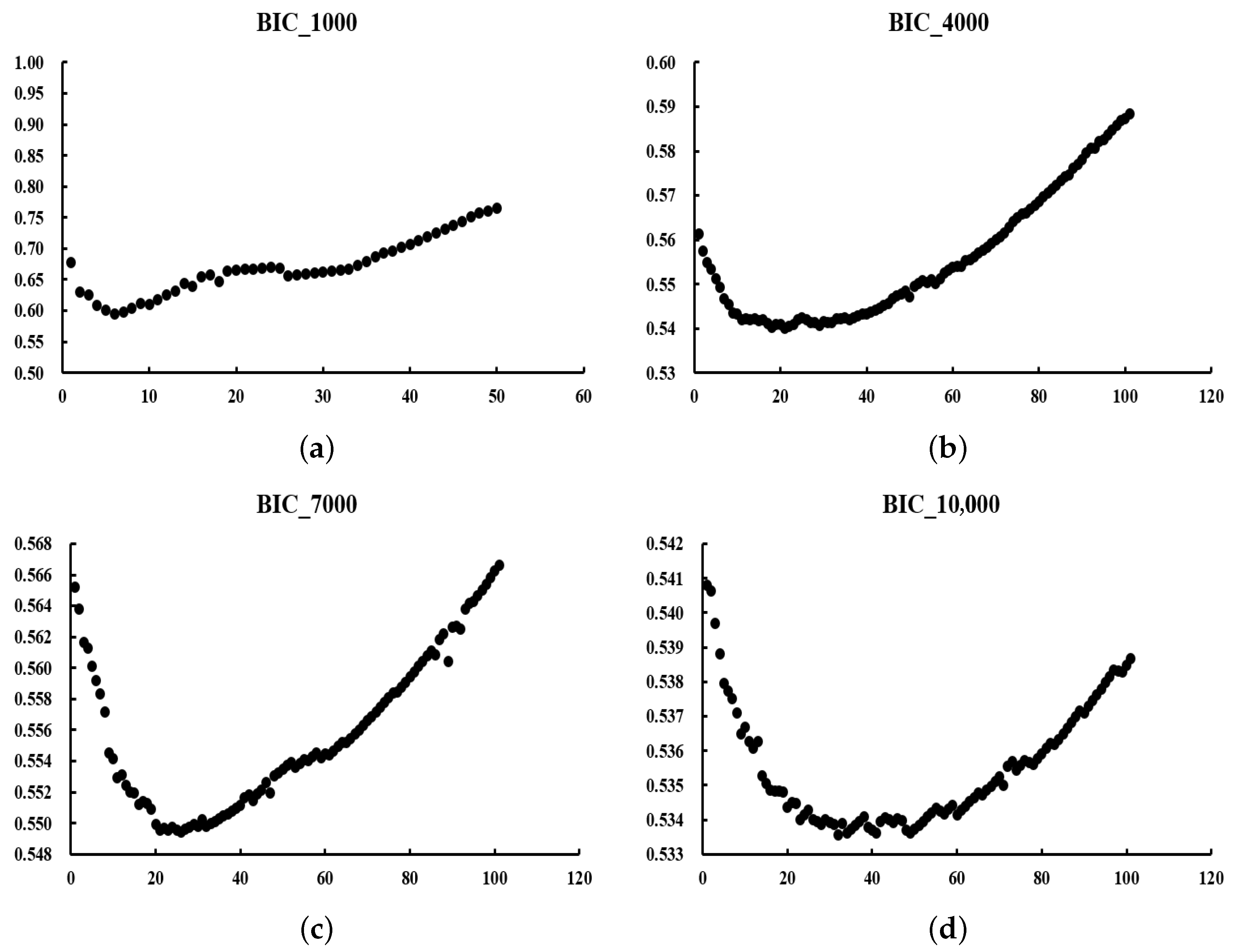
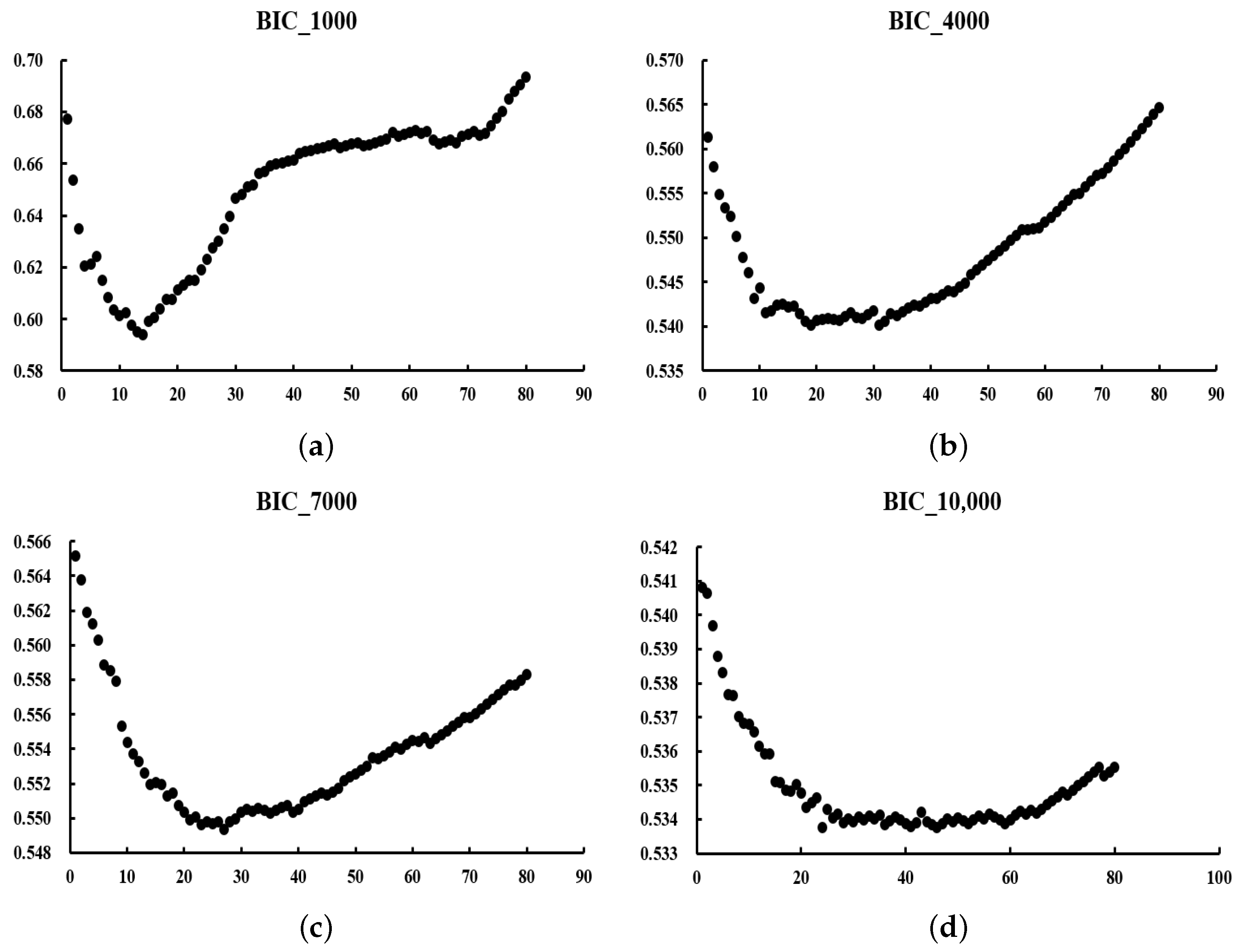
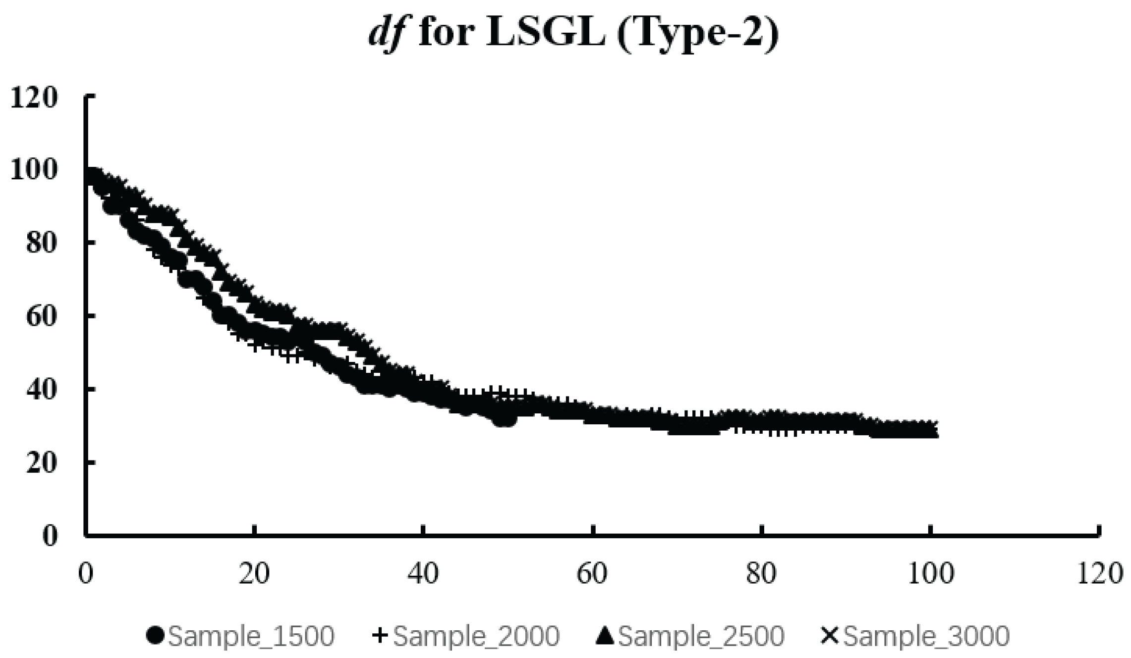
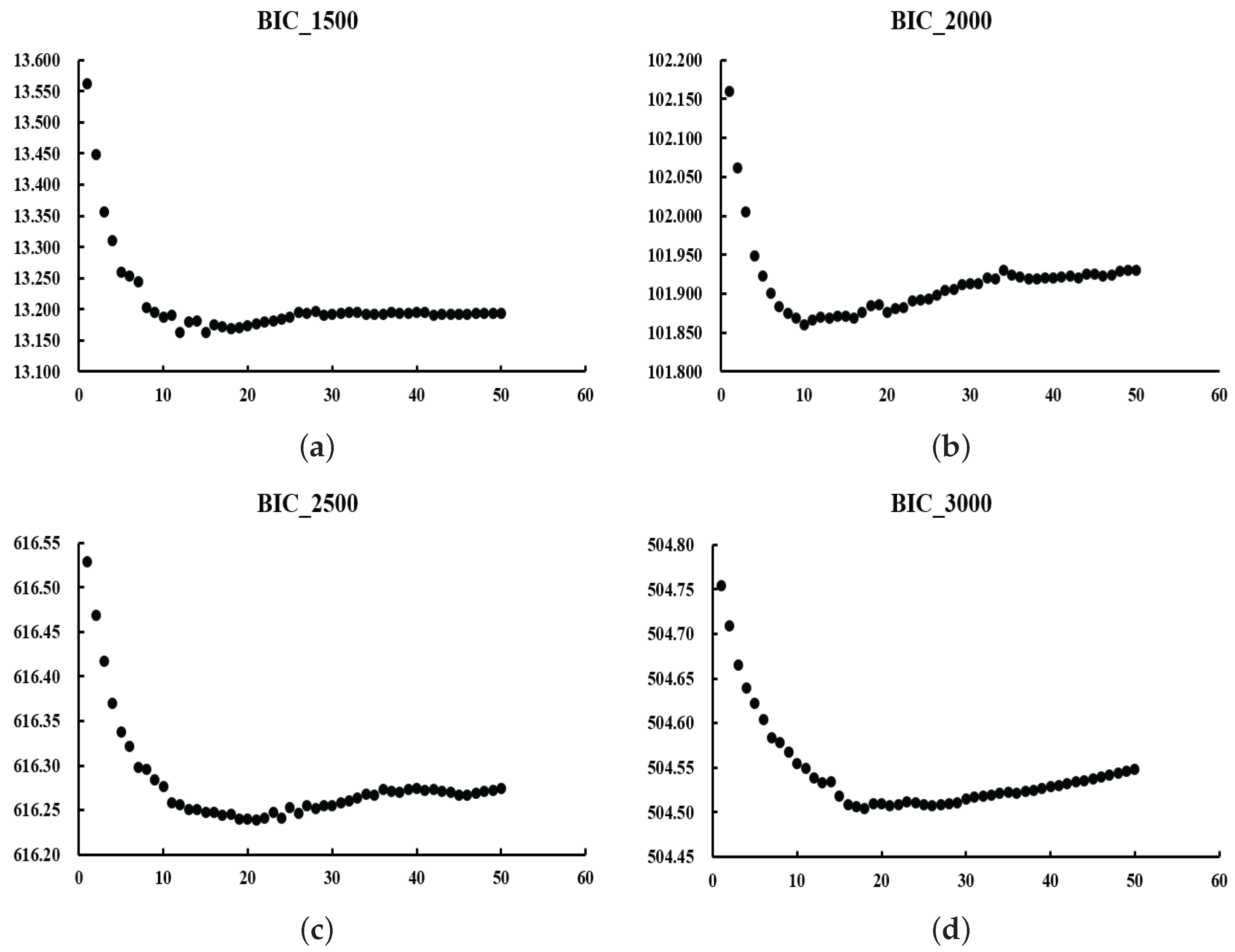
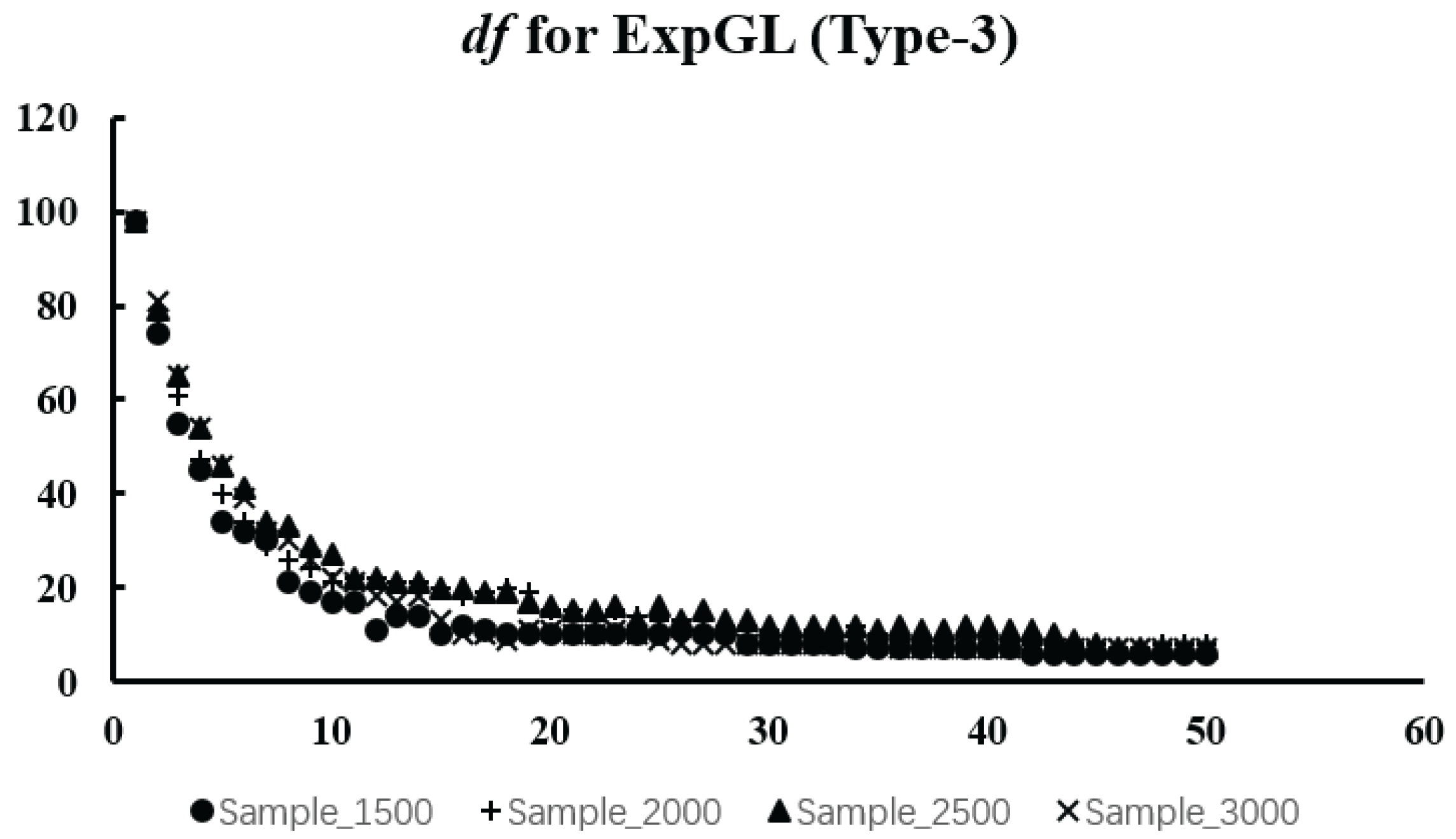
3.3. Choice of $\lambda$

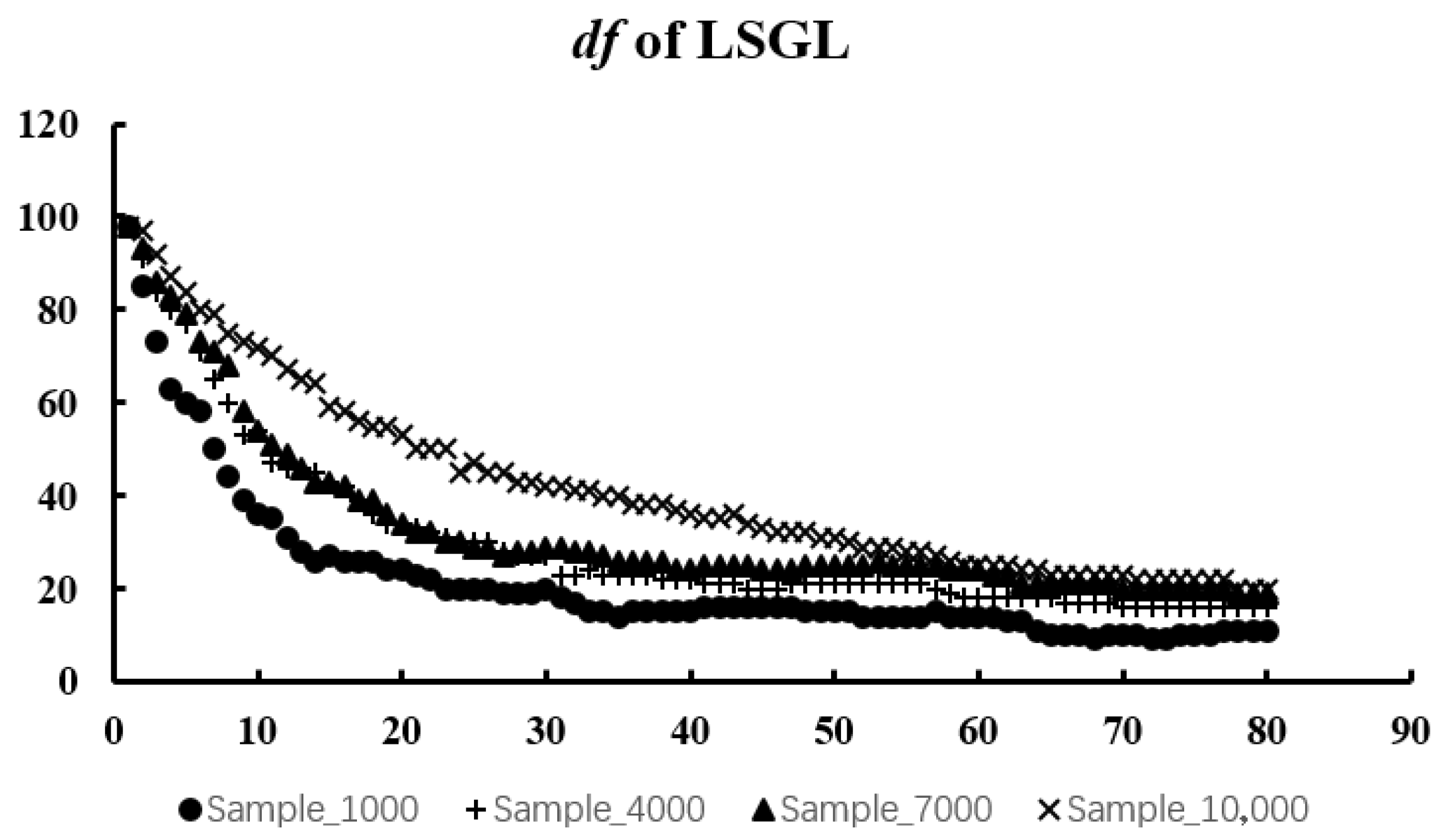
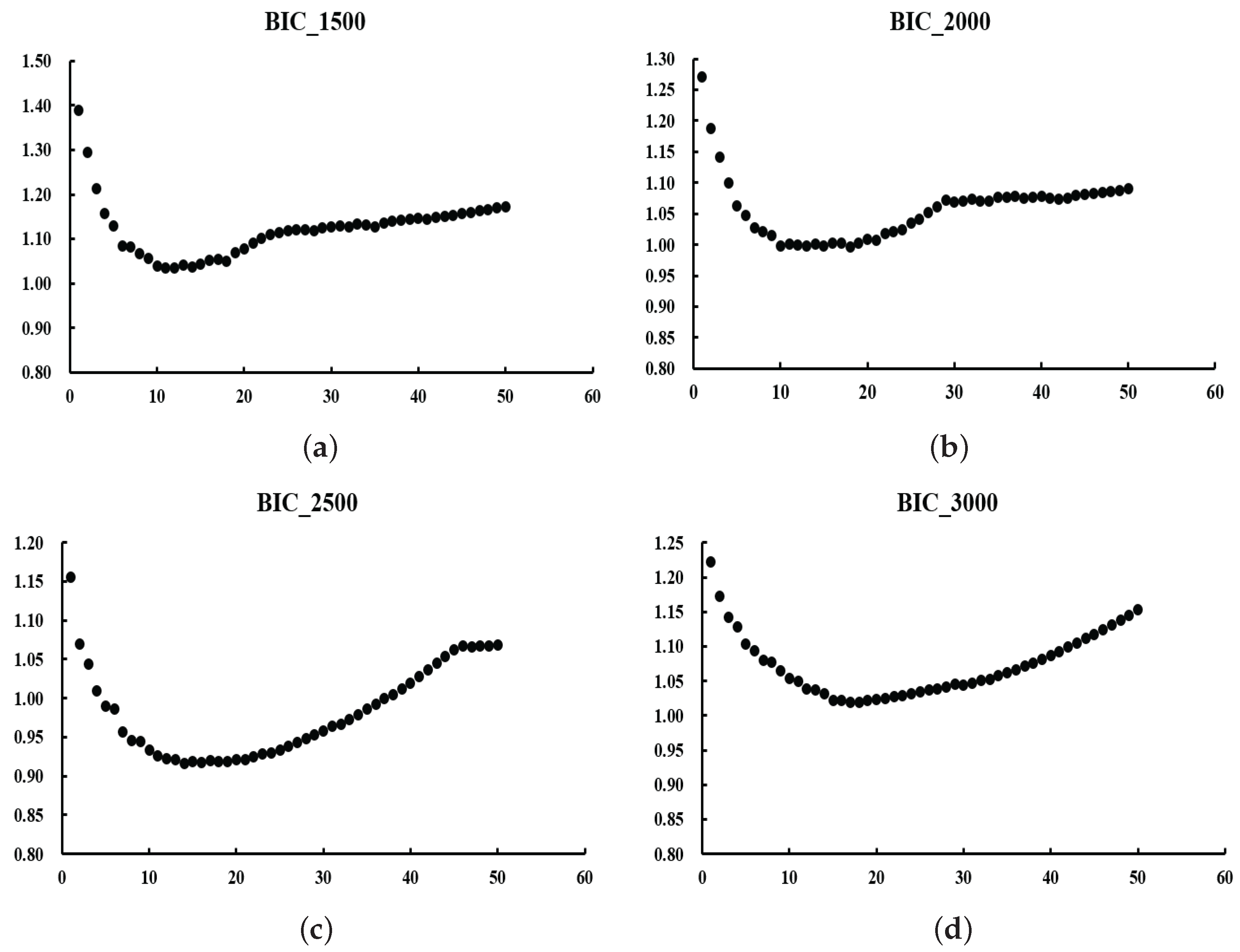
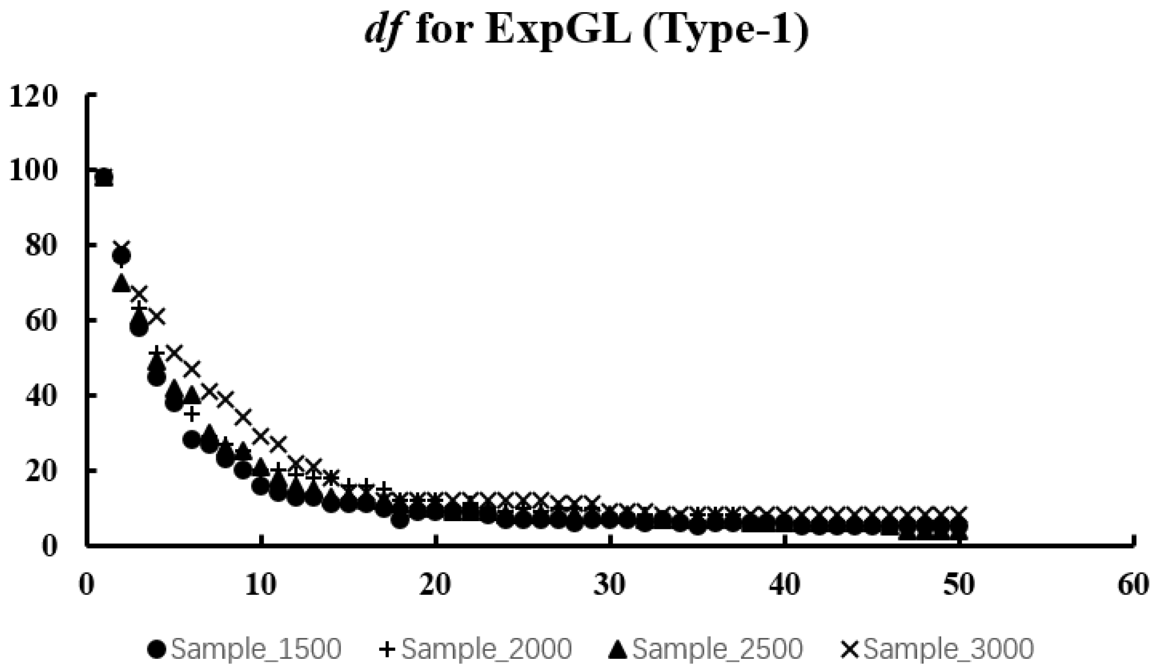
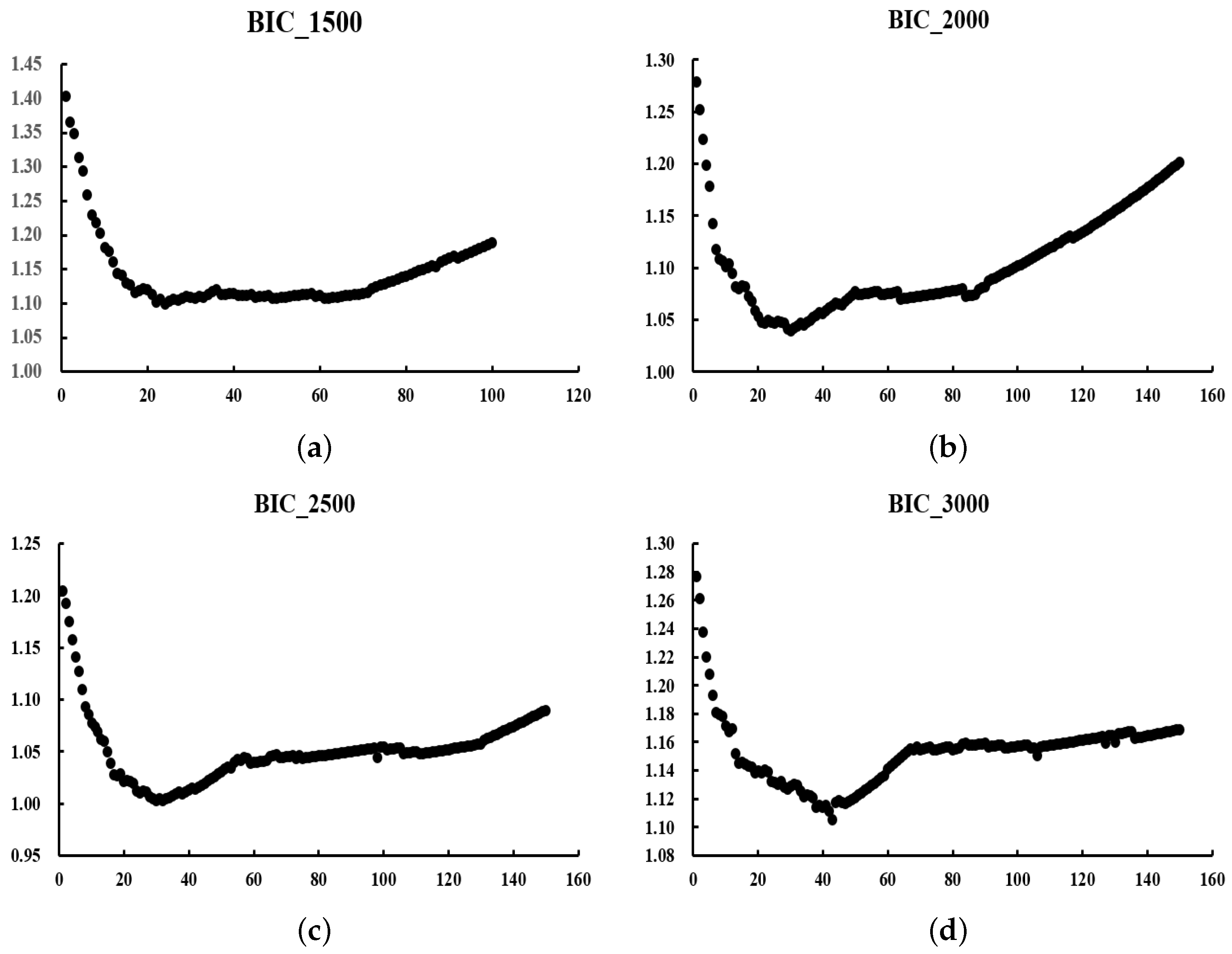
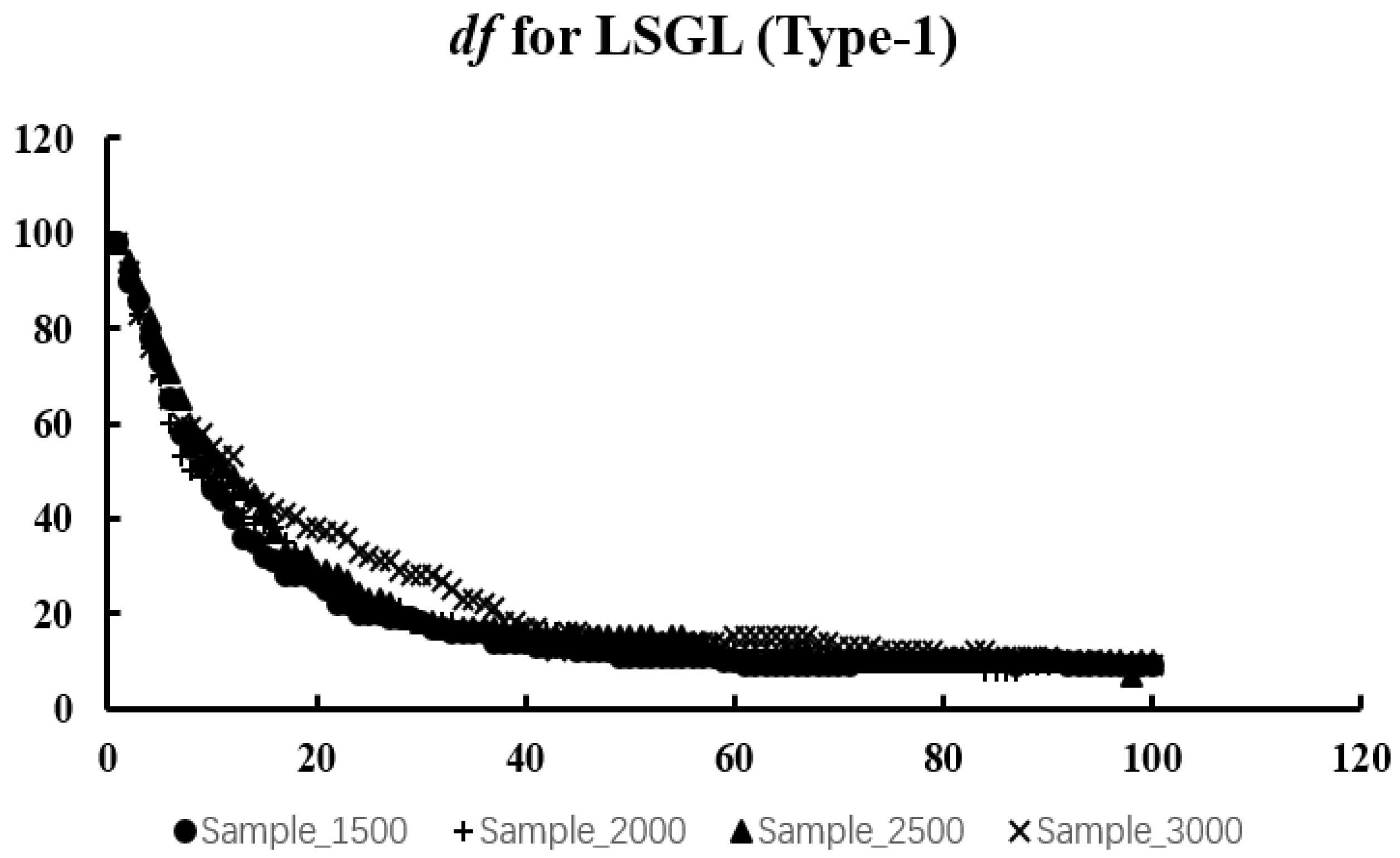
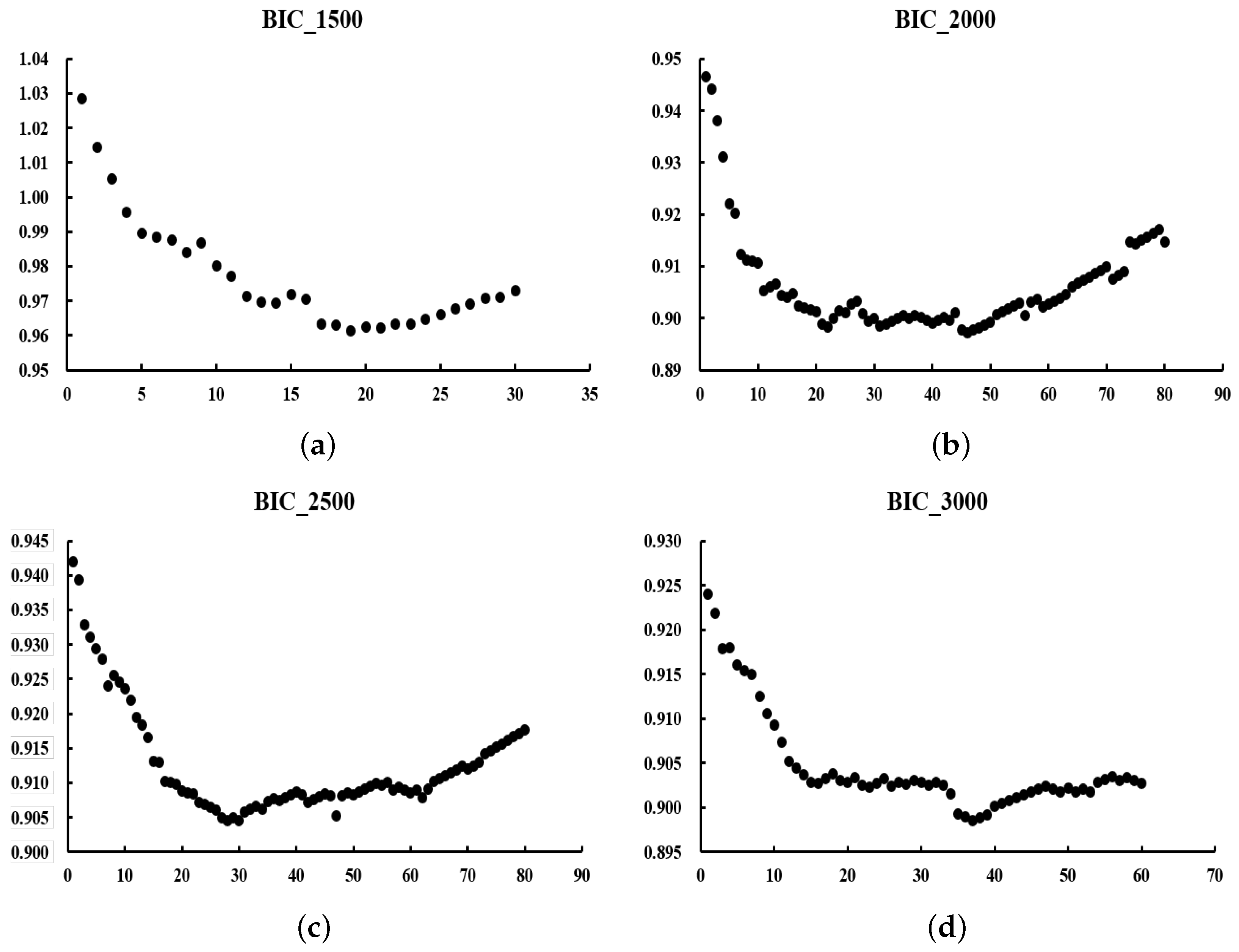
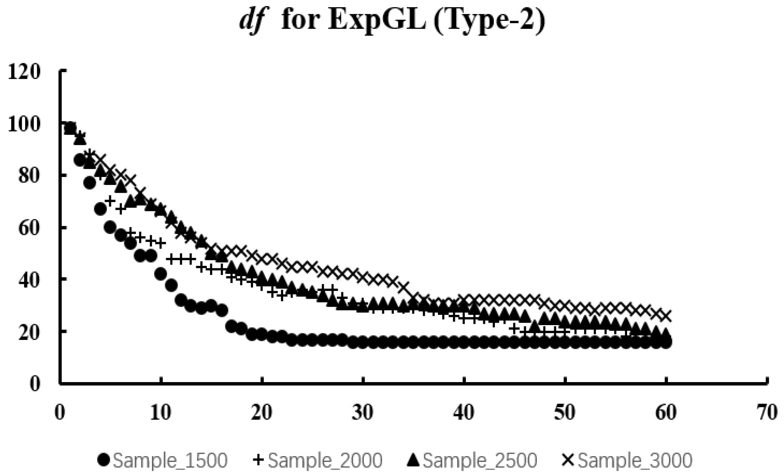
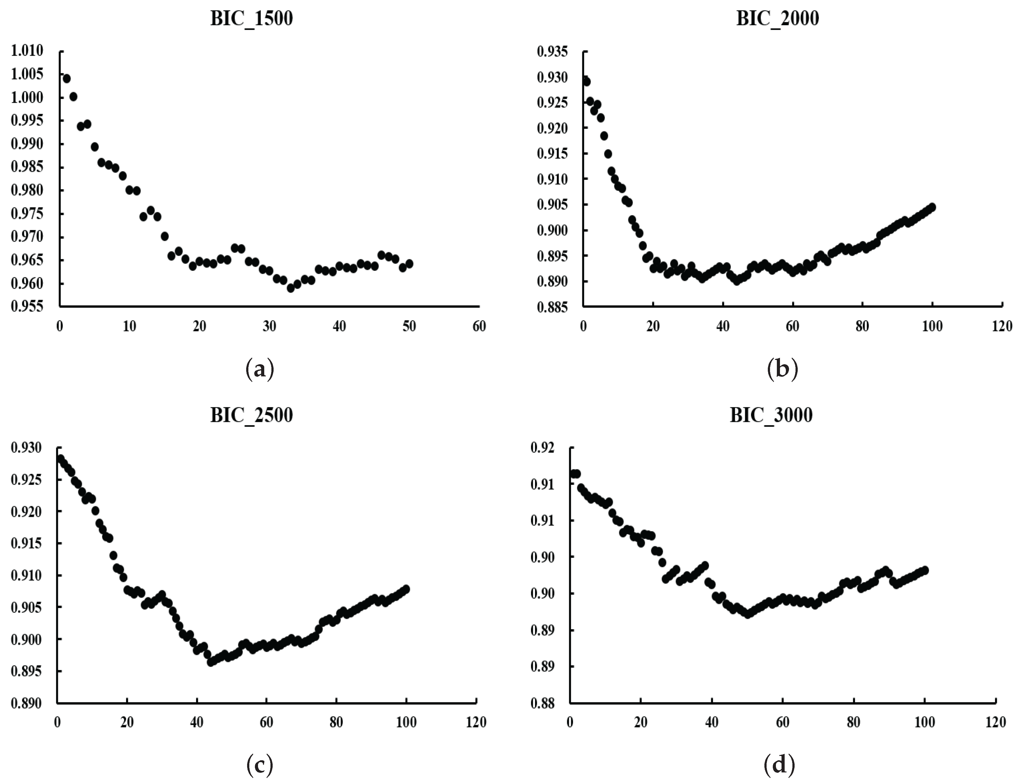
First, we determine the interval for selecting $\lambda$. Then, we select an appropriate length and obtain a series of $\lambda$ values from the interval, which is called as set R. For any ${\lambda }_i\in R$, we calculate the degrees of freedom and the $BIC$ value using the following formula:

$$BIC(\widehat{Y})={\displaystyle \frac{\parallel Y-\widehat{Y}{\parallel }_2^2}{n{\sigma }^2}}+{\displaystyle \frac{log\left(n\right)}{n}}df(\widehat{Y}).$$

We expect to obtain a U-shaped curve of $BIC$ values. The $\lambda$ at the curve’s lowest point represents the optimal value. The reason for choosing the $BIC$ criterion is that it requires less computation than the optimal $\lambda$ value obtained by cross-validation.

In the next section, we will discuss numerical simulations and real-data experiments using the algorithm given in this section.

4. Simulation and Result Analysis

Up to now, we have presented our model’s construction process, the parameter calculation methods, and solution algorithm. In this section, we will first implement the algorithm described in the previous sections using Matlab [22]. Next, key model parameters are estimated using simulated and real data. Finally, model evaluation is performed based on these parameters.

4.1. Numerical Simulation Experiment

In this part, we consider two basic cases of data with and without outliers. We will choose a model for comparison, which is also a variable selection method with penalty function under linear constraints based on the least squares loss [14].

4.1.1. Sample Without Outliers

First, let us look at the process of generating simulation data without outliers. The basic model is as follows:

$$Y=X\beta +ϵ.$$

where $\beta ={(1,0.5,-1,0,\dots ,0,1,0.5,-1,0,\dots ,0)}^{\prime }$ and ${ϵ}_i\stackrel{\mathrm{i}.\mathrm{i}.\mathrm{d}}{\sim }N(0,2.0^2)$. The dimension of $\beta$ is 100. Simultaneously, there are six non-zero elements in $\beta$ located at positions 1, 2, 3, 11, 12, and 13. In addition, $X_i\sim N(\mathbf{0},\Omega )$, where $\mathbf{0}\in {\mathbb{R}}^{100}$ and ${\Omega }_{ij}=0.5^{|i-j|}$.

In this paper, we consider the problem of parameter estimation and variable selection with linear constraints; the loss function is the exponential squared loss and the penalty term is generalized Lasso. In the simulation experiment, we chose one case in which the penalty term satisfies the fused lasso. The penalty function is shown below:

$$\lambda \sum _{k=1}^{100}|{\beta }_k|+\lambda \sum _{k=2}^{100}|{\beta }_k-{\beta }_{k-1}|.$$

In the case that the penalty term satisfies the fused lasso, the matrix D in Equation (5) is

$${\left(\begin{array}{ccccc}-1& 1& 0\dots & 0& 0\\ 0& -1& 1\dots & 0& 0\\ & \dots \\ 0& 0& 0\dots & -1& 1\end{array}\right)}_{99\times 100}$$

The linear constraints are

$$\begin{array}{cc}\hfill {\beta }_1+{\beta }_2+{\beta }_3& \ge 0,\hfill \\ \hfill {\beta }_2+{\beta }_5+{\beta }_{11}& \ge 1,\hfill \\ \hfill {\beta }_1+{\beta }_3+{\beta }_{11}+{\beta }_{13}& =0,\hfill \\ \hfill {\beta }_2+{\beta }_8+{\beta }_{12}& =1.\hfill \end{array}$$

Here, the parameter settings and constraints employed in the simulations are based on the work of Wu et al. [18]. To facilitate the following discussion, we denote the variable selection method based on generalized Lasso and exponential squared loss under linear constraints as ExpGL. Similarly, the variable selection method based on generalized Lasso and least squares loss under linear constraints [14] is denoted as LSGL. We designed four numerical experiments with sample sizes of 1000, 4000, 7000, and 10,000, performing 50 repeated trials for each sample size. For each group of experiment, we apply both ExpGL and LSGL methods to calculate $BIC$, $df$, $MSE$, $MAE$, $PSR$ (positive selection rate), and $FDR$ (false discovery rate). $BIC$ is used to select the optimal $\lambda$ and thus determines the corresponding coefficient estimate $\beta$. $df$ is used to measure the complexity of the model. $MSE$ and $MAE$ are used to evaluate the accuracy of ExpGL and LSGL in coefficient estimation. $PSR$ and $FDR$ are used to evaluate the presence of over-selected or missed valid variables [23].

This paper presents some results from our numerical simulations, which are shown below.

Figure 2 and Figure 3 show distinct U-shaped curves, which is in line with our expectations. If we fit the U-shaped curve to minimize the value, then we will obtain the optimal $\lambda$. In Figure 4 and Figure 5, the degrees of freedom decrease with the gradual increase in $\lambda$. As $\lambda$ increases, the sparsity of the model becomes stronger, which then leads to the emergence of a simpler model that is finally reflected as the gradual decrease in $df$ (degrees of freedom).

Table 1. Performance metrics of ExpGL and LSGL methods across varying sample sizes.

Sample	Method	${\mathit{\lambda }}_{\mathit{opt}}$	$\mathit{df}$	$\mathit{MSE}$	$\mathit{MAE}$	$\mathit{PSR}$	$\mathit{FDR}$
1000	LSGL	57.0895	30	4.0914	1.6212	1.000	0.25
	ExpGL	1.0387	28	4.0980	1.6226	1.000	0.40
4000	LSGL	105.9475	31	4.1197	1.6122	1.000	0.25
	ExpGL	3.9100	32	4.1185	1.6118	1.000	0.25
7000	LSGL	130.4245	27	3.9601	1.5874	1.000	0.25
	ExpGL	4.9712	27	3.9603	1.5874	1.000	0.25
10,000	LSGL	233.1305	32	3.9348	1.5854	1.000	0.25
	ExpGL	7.4606	37	3.9285	1.5836	1.000	0.25

below summarizes the performance of ExpGL and LSGL under different sample sizes using the optimal $\lambda$ obtained from the BIC criterion. Based on the results in Table 1, the following conclusions can be drawn:

1.

From the perspective of $df$, the model obtained by LSGL is relatively simple because its degrees of freedom with the increase in sample size is always smaller than that of the ExpGL method.

2.

In terms of $MSE$ and $MAE$, their estimates of coefficients are not significantly different, which means both methods provide good estimates of the real model.

3.

Based on these $PSR$ and $FDR$ values, we can determine that both the ExpGL and LSGL methods successfully identified all the real valid variables. According to these values of $FDR$, it can be found that the estimates of effective variables obtained by the two methods differ little.

When no outliers are present, both variable selection methods provide final models that can effectively estimate the true model. Nevertheless, LSGL is preferable in this outlier-free scenario since it generates a simpler model with faster computational speed.

4.1.2. Sample with Outliers

In this paper, the model is expected to have certain robustness in the face of data with certain noise points or outliers. Therefore, this part is mainly to verify the noise resistance ability of our model. Outliers can exist only in the explanatory variable X, in the response variable Y, or in both.

The original data follow the data generation rules in Section 4.1.1. According to X. Wang et al. [10], the data without outliers can be transformed into data with noise points in the following three ways:

Type-1. Outliers in the predictors

$X_i$ follows the d-dimensional mixed normal distribution, which is shown below:

$$X_i\sim 0.8N(\mathbf{0},\tilde{\Omega })+0.2N(\mathit{\mu },\Omega ).$$

where $\tilde{\Omega }=I_{d\times d}$ and $\mathit{\mu }=3{\mathbf{1}}_d$. The parameter d is set to 100 in this study, which is the same as that in Section 4.1.1—this information will not be repeated later. In addition, ${ϵ}_i\stackrel{\mathrm{i}.\mathrm{i}.\mathrm{d}}{\sim }N(0,2.0^2)$.

Type-2. Outliers in the response

$X_i$ follows the d-dimensional normal distribution, which is shown below:

$$X_i\sim N(\mathbf{0},\Omega ).$$

${ϵ}_i$ follows the mixed normal distribution, which is shown below:

$$ϵ\sim 0.8N(0,1)+0.2N(10,6^2).$$

Type-3. Outliers in both the predictors and response

$X_i$ follows the d-dimensional mixed normal distribution, which is shown below:

$$X_i\sim 0.8N(\mathbf{0},\tilde{\Omega })+0.2N(\mathit{\mu },\Omega ).$$

At the same time, ${ϵ}_i$ follows a Cauchy distribution.

For each type, we designed four samples with different sizes (1500, 2000, 2500, and 3000). Below are some results for the three different types of outliers.

Based on the analysis of Figure 6, Figure 7, Figure 8, Figure 9, Figure 10, Figure 11, Figure 12, Figure 13, Figure 14 and Figure 15 and

Table 2. ExpGL and LSGL (Type-1).

Sample	Method	${\mathit{\lambda }}_{\mathit{opt}}$	$\mathit{df}$	$\mathit{MSE}$	$\mathit{MAE}$	$\mathit{PSR}$	$\mathit{FDR}$
1500	LSGL	95	20	3.1757	1.3464	1.000	0.54
	ExpGL	5	14	1.2618	0.9063	1.000	0.33
2000	LSGL	125	23	3.1876	1.3371	1.000	0.57
	ExpGL	6	18	1.2327	0.8918	1.000	0.33
2500	LSGL	145	18	3.0470	1.3071	1.000	0.68
	ExpGL	7.5	13	1.1205	0.8431	1.000	0.40
3000	LSGL	220	12	3.2550	1.3674	1.000	0.14
	ExpGL	8	12	1.2134	0.8860	1.000	0.14

,

Table 3. ExpGL and LSGL (Type-2).

Sample	Method	${\mathit{\lambda }}_{\mathit{opt}}$	$\mathit{df}$	$\mathit{MSE}$	$\mathit{MAE}$	$\mathit{PSR}$	$\mathit{FDR}$
1500	LSGL	64	41	0.3573	0.4753	1.000	0.78
	ExpGL	1.8	19	0.2592	0.4071	1.000	0.14
2000	LSGL	66	43	0.2889	0.4303	1.000	0.81
	ExpGL	4.5	20	0.1490	0.3096	1.000	0.33
2500	LSGL	86	36	0.1923	0.3510	1.000	0.76
	ExpGL	2.9	30	0.1012	0.2528	1.000	0.40
3000	LSGL	100	41	0.1486	0.3050	1.000	0.86
	ExpGL	3.6	31	0.0754	0.2210	1.000	0.25

and

Table 4. ExpGL (Type-3) *.

Sample	Method	${\mathit{\lambda }}_{\mathit{opt}}$	$\mathit{df}$	$\mathit{MSE}$	$\mathit{MAE}$	$\mathit{PSR}$	$\mathit{FDR}$
1500	ExpGL	7	10	1.1543	0.8682	1.000	0.33
2000	ExpGL	4.5	21	1.0659	0.8424	1.000	0.33
2500	ExpGL	10	15	1.2022	0.87367	1.000	0.25
3000	ExpGL	8.5	9	1.1545	0.86611	1.000	0.25

* In this scenario, no matter how large the sample size is, the LSGL method always fails to select the appropriate penalty parameters. For example, when the sample size is 1500, the resulting MSE and MAE values are 958 and 24, respectively. For the above reasons, the final results obtained by the LSGL method are not shown here.

, we can obtain the following results:

• In each case, the $BIC$ curve is U-shape, so we can indeed select the optimal $\lambda$ value according to the $BIC$ curve. Compared with the cross-validation method, this approach of parameter selection is easier to operate and can also lead to the desired result.
• Across all cases, the $MSE$ and $MAE$ values of the model obtained by the ExpGL method are lower than those calculated by LSGL. Particularly, considering the third outlier type (Table 4), LSGL fails to provide the correct model. However, our proposed method can produce a better estimate of the real model.
• According to the $PSR$ and $FDR$ values in different cases, we can conclude that our model can select all real valid variables, and the estimated number of valid variables is much smaller than that obtained by LSGL. Furthermore, increasing $\lambda$ progressively reduces model complexity, as reflected by decreasing degrees of freedom.

To sum up, regardless of the type of outliers, ExpGL performs better than LSGL. Even with outliers present, ExpGL still maintains satisfactory variable selection and estimation capabilities. Especially in the third type of outliers, LSGL fails to provide the correct model, while ExpGL can still obtain a prediction model close to the real model.

4.2. Real-Data Experiments

In this section, we first choose the Boston Housing Price Dataset as a sample. Then, we apply our model to this dataset. Finally, we analyze the results. This dataset was originally proposed by Harrison Jr and Rubinfeld [24] and has been widely used as a benchmark dataset in numerous studies.

Table 5. Variables in dataset.

	Variable	Meaning
Explanatory Variables	CRIM	per capita crime rate by town
	ZN	proportion of residential land zoned for lots over 25,000 sq.ft.
	INDUS	proportion of non-retail business acres per town
	CHAS	Charles River dummy variable (=1 if tract bounds river; 0 otherwise)
	NOX	nitric oxide concentration (parts per 10 million)
	RM	average number of rooms per dwelling
	AGE	proportion of owner-occupied units built prior to 1940
	DIS	weighted distances to five Boston employment centers
	RAD	index of accessibility to radial highways
	TAX	full-value property-tax rate per USD 10,000
	PTRATIO	pupil/teacher ratio by town
	B	1000(Bk − 0.63)⌃2, where Bk is the proportion of blacks by town
	LSTAT	% lower status of the population
Response Variable	MEDV	median value of owner-occupied homes in USD 1000’s

shows the names and meanings of variables in the dataset. This dataset comprises 506 samples with 13 explanatory variables and 1 response variable. Key statistics include the following: CRIM with mean 3.61, standard deviation (SD) 8.60, and range 0.006 88.98; RM with mean 6.28, SD 0.70, and range 3.56–8.78; and LSTAT with mean 12.65, SD 7.14, range 1.73–37.97. The target variable MEDV has a mean of 22.53, SD 9.20, ranging from 5.0 to 50.0. In addition, notable features include PTRATIO with mean 18.46, AGE with mean 68.57, and so on. The data exhibit heteroscedasticity, with strong correlations between variables like RM/LSTAT and MEDV. Note that the values described here for the data features are rounded to two decimal places.

First, the dataset is standardized with a mean value of 0 and variance of 1. Next, we build the following model:

$$\begin{array}{cc}\hfill \underset{\beta }{min}& \sum _{i=1}^n\{1-exp\{-{\displaystyle \frac{{(Y_i-x_i^T\beta )}^2}{\gamma }}\}\}+\lambda {\parallel \beta \parallel }_1,\hfill \\ \hfill \mathrm{s}.\mathrm{t}.& {\beta }_1<0.001,{\beta }_2<0.001,{\beta }_8<0.001,{\beta }_{12}<0.001,\hfill \\ & {\beta }_3+{\beta }_5+{\beta }_6+{\beta }_{12}=0.6.\hfill \end{array}$$

where the limitations of linear constraints are actually set according to the results obtained by some scholars [10]. Then, the method proposed in this paper is used to obtain the estimation of $\beta$; the results are presented below. Moreover, we calculate that the values of MSE and MAE are 0.377 and 0.397, respectively, while the value of $R^2$ is greater than 0.9.

From

Table 6. Estimated regression coefficients from the dataset.

Explanatory Variables

CRIM

ZN

INDUS

CHAS

NOX

RM

AGE

DIS

RAD

TAX

PTRATIO

B

LSTAT

Estimation by ExpGL

0

0

0

0

0

0.601

−0.026

0

0

−0.116

−0.1

0

−0.128

, it can be found that the final estimated coefficient value conforms to the linear constraint conditions set earlier. At the same time, it can also be confirmed that the model does have good variable selection ability, as only five significant variables were chosen. Finally, we know that most common regression models—such as linear regression and ridge regression, among others—typically achieve $R^2$ values between 0.7 and 0.9. Similar to MSE and MAE, the R² value also indicates that the estimated model is a good characterization of the original model.

So far, we have discussed the performance of the model with and without outliers and evaluated it using actual data. In the following section, we summarize the work of this article and present a discussion.

5. Discussion

The main purpose of this paper is to design a robust variable selection method combining prior information. In order to ensure robustness, that is, to resist the influence of certain abnormal or noise points, we chose the exponential squared loss function as the loss under a penalized likelihood framework. Simultaneously, in order to obtain a more realistic model, we considered adding some prior information to the variable selection method through linear constraints. Finally, we constructed an optimization problem with the linear constraints. Since the objective function is non-convex, it is not easy to deal with. Therefore, we employed Taylor expansion to transform the model into a more tractable quadratic programming problem. Then, in order to deal with the transformed model more easily by using the coordinate descent method, we obtained the dual form of the quadratic programming problem first. Finally, the estimation of the final coefficient was obtained by applying the coordinate descent method to the dual problem. Note that some parameter selections were involved in the process, but we will not repeat them here.

After the algorithm was obtained, numerical simulations and real-data experiments were carried out. The experimental results show that the performance of our method without outliers is not significantly different from that of LSGL, but the latter is easier to operate. When outliers are present, our method significantly outperforms LSGL. In the third outlier scenario, LSGL is no longer effective, but our method maintains satisfactory performance. Our method demonstrates effective handling of outliers in the predictors, outliers in the response, as well as scenarios involving both. These results suggest that our method is indeed robust. Furthermore, as established in the work of X. Wang et al. [10], the breakdown point (BP) is fundamentally determined by the breakdown point of the initial estimate and the tuning parameter $\gamma$. The results of the real-data experiments show that the coefficients estimated by our method meet the linear constraints set previously, and the sparse model can be obtained by compressing variables. In other words, both numerical simulations and real-data experiments show that our method conforms to the expectations established.

So far, there is little research on the oracle properties of variable selection models under linear constraints. For future research, in addition to the model proposed in this paper, we intend to uniformly prove the oracle properties of all variable selection models proposed so far under linear constraints, for example, variable selection models based on least squares loss under linear constraints, variable selection models based on quantile loss under linear constraints, and so on.

References

1. Tibshirani, R. Regression shrinkage and selection via the lasso. J. R. Stat. Soc. Ser. B (Methodol.) 1996, 58, 267–288. [Google Scholar] [CrossRef]
2. Tibshirani, R.; Saunders, M.; Rosset, S.; Zhu, J.; Knight, K. Sparsity and smoothness via the fused lasso. J. R. Stat. Soc. Ser. B (Stat. Methodol.) 2005, 67, 91–108. [Google Scholar] [CrossRef]
3. Zou, H. The adaptive lasso and its oracle properties. J. Am. Stat. Assoc. 2006, 101, 1418–1429. [Google Scholar] [CrossRef]
4. Zou, H.; Hastie, T. Regularization and variable selection via the elastic net. J. R. Stat. Soc. Ser. B (Stat. Methodol.) 2005, 67, 301–320. [Google Scholar] [CrossRef]
5. Bahrami, K.; Kot, A.C. A fast approach for no-reference image sharpness assessment based on maximum local variation. IEEE Signal Process. Lett. 2014, 21, 751–755. [Google Scholar] [CrossRef]
6. Tibshirani, R.J. The solution path of the generalized lasso. Ann. Stat. 2011, 39, 1335–1371. [Google Scholar] [CrossRef]
7. Fan, J.; Li, R. Variable selection via nonconcave penalized likelihood and its oracle properties. J. Am. Stat. Assoc. 2001, 96, 1348–1360. [Google Scholar] [CrossRef]
8. Wang, H.; Li, G.; Jiang, G. Robust regression shrinkage and consistent variable selection through the LAD-Lasso. J. Bus. Econ. Stat. 2007, 25, 347–355. [Google Scholar] [CrossRef]
9. Wu, Y.; Liu, Y. Variable Selection in Quantile Regression. Stat. Sin. 2009, 19, 801–817. [Google Scholar]
10. Wang, X.; Jiang, Y.; Huang, M.; Zhang, H. Robust variable selection with exponential squared loss. J. Am. Stat. Assoc. 2013, 108, 632–643. [Google Scholar] [CrossRef]
11. Fan, J.; Lv, J. A selective overview of variable selection in high dimensional feature space. Stat. Sin. 2010, 20, 101. [Google Scholar] [PubMed]
12. Fan, J.; Zhang, J.; Yu, K. Vast portfolio selection with gross-exposure constraints. J. Am. Stat. Assoc. 2012, 107, 592–606. [Google Scholar] [CrossRef] [PubMed]
13. Wang, J.; Ghosh, S.K. Shape restricted nonparametric regression with Bernstein polynomials. Comput. Stat. Data Anal. 2012, 56, 2729–2741. [Google Scholar] [CrossRef]
14. Hu, Q.; Zeng, P.; Lin, L. The dual and degrees of freedom of linearly constrained generalized lasso. Comput. Stat. Data Anal. 2015, 86, 13–26. [Google Scholar] [CrossRef]
15. Liu, Y.; Zeng, P.; Lin, L. Generalized l1-penalized quantile regression with linear constraints. Comput. Stat. Data Anal. 2020, 142, 106819. [Google Scholar] [CrossRef]
16. Yang, J.; Tian, G.; Lu, F.; Lu, X. Single-index modal regression via outer product gradients. Comput. Stat. Data Anal. 2020, 144, 106867. [Google Scholar] [CrossRef]
17. Friedman, J.; Hastie, T.; Tibshirani, R. Additive logistic regression: A statistical view of boosting (with discussion and a rejoinder by the authors). Ann. Stat. 2000, 28, 337–407. [Google Scholar] [CrossRef]
18. Wu, W.; Guo, Y.; Zhang, B.; Bose, A.; Hongbin, S. Robust state estimation method based on maximum exponential square. IET Gener. Transm. Distrib. 2011, 5, 1165–1172. [Google Scholar] [CrossRef]
19. Boyd, S.P.; Vandenberghe, L. Convex Optimization; Cambridge University Press: Cambridge, UK, 2004. [Google Scholar]
20. Stein, C.M. Estimation of the mean of a multivariate normal distribution. Ann. Stat. 1981, 9, 1135–1151. [Google Scholar] [CrossRef]
21. Efron, B. The estimation of prediction error: Covariance penalties and cross-validation. J. Am. Stat. Assoc. 2004, 99, 619–632. [Google Scholar] [CrossRef]
22. Haigang Kang, B.D. Matlab for Data Analysis; China Machine Press: Beijing, China, 2021. [Google Scholar]
23. Chen, J.; Chen, Z. Extended Bayesian information criteria for model selection with large model spaces. Biometrika 2008, 95, 759–771. [Google Scholar] [CrossRef]
24. Harrison, D., Jr.; Rubinfeld, D.L. Hedonic housing prices and the demand for clean air. J. Environ. Econ. Manag. 1978, 5, 81–102. [Google Scholar] [CrossRef]
Figure 1. Exponential loss function ϕ γ ( t ) , where γ = 1 . Figure (a) shows the overall image of the Exponential loss function, and Figure (b) shows the image of interval 2.4 to 4 in detail. These two graphs demonstrate the robustness of the exponential squared loss function to outliers.
Axioms 14 00516 g001
Figure 2. B I C for ExpGL (the relation between horizontal axis x and λ is λ = 0.2 × ( x 1 ) ). This shows optimal λ selection via U-shaped curves. Figures (ad) show the results for sample sizes of 1000, 4000, 7000 and 10,000, respectively.
Axioms 14 00516 g002
Figure 3. B I C for LSGL (the relation between horizontal axis x and λ is λ = 5 × ( x 1 ) ). Figures (ad) show the results for sample sizes of 1000, 4000, 7000 and 10,000, respectively.
Axioms 14 00516 g003
Figure 4. d f for ExpGL (the relation between horizontal axis x and λ is λ = 0.2 × ( x 1 ) ). This shows the regulatory effect of λ on model complexity.
Axioms 14 00516 g004
Figure 5. d f for LSGL (the relation between horizontal axis x and λ is λ = 5 × ( x 1 ) ).
Axioms 14 00516 g005
Figure 6. B I C for ExpGL (Type-1) (the relation between horizontal axis x and λ is λ = 0.5 × ( x 1 ) ). Figures (ad) show the results for sample sizes of 500, 2000, 2500, and 3000, respectively.
Axioms 14 00516 g006
Figure 7. d f for ExpGL (Type-1) (the relation between horizontal axis x and λ is λ = 0.5 × ( x 1 ) ).
Axioms 14 00516 g007
Figure 8. B I C for LSGL (Type-1) (the relation between horizontal axis x and λ is λ = 5 × ( x 1 ) ). Figures (ad) show the results for sample sizes of 500, 2000, 2500, and 3000, respectively.
Axioms 14 00516 g008
Figure 9. d f for LSGL (Type-1) (the relation between horizontal axis x and λ is λ = 5 × ( x 1 ) ).
Axioms 14 00516 g009
Figure 10. B I C for ExpGL (Type-2) (the relation between horizontal axis x and λ is λ = 0.1 × ( x 1 ) ). Figures (ad) show the results for sample sizes of 500, 2000, 2500, and 3000, respectively.
Axioms 14 00516 g010
Figure 11. d f for ExpGL (Type-2) (the relation between horizontal axis x and λ is λ = 0.1 × ( x 1 ) ).
Axioms 14 00516 g011
Figure 12. B I C for LSGL (Type-2) (the relation between horizontal axis x and λ is λ = 2 × ( x 1 ) ). Figures (ad) show the results for sample sizes of 500, 2000, 2500, and 3000, respectively.
Axioms 14 00516 g012
Figure 13. d f for LSGL (Type-2) (the relation between horizontal axis x and λ is λ = 2 × ( x 1 ) ).
Axioms 14 00516 g013
Figure 14. B I C for ExpGL (Type-3) (the relation between horizontal axis x and λ is λ = 0.5 × ( x 1 ) ). Figures (ad) show the results for sample sizes of 500, 2000, 2500, and 3000, respectively.
Axioms 14 00516 g014
Figure 15. d f for ExpGL (Type-3) (the relation between horizontal axis x and λ is λ = 0.5 × ( x 1 ) ).
Axioms 14 00516 g015