Article

Optimizing Parameter Estimation Precision in Open Quantum Systems

Department of Physics, College of Science, Imam Mohammad Ibn Saud Islamic University (IMSIU), Riyadh 11623, Saudi Arabia
Axioms 2025, 14(5), 368; https://doi.org/10.3390/axioms14050368
Submission received: 27 February 2025 / Revised: 22 April 2025 / Accepted: 29 April 2025 / Published: 13 May 2025
(This article belongs to the Special Issue Applied Nonlinear Dynamical Systems in Mathematical Physics)

Abstract

:
In the present manuscript, we demonstrate the potential to control and enhance the accuracy of parameter estimation (P-E) in a two-level atom (TLA) immersed in a cavity field that interacts with another cavity. We investigate the dynamics of quantum Fisher information (FI), considering the influence of coupling strength between the two cavities and the detuning parameter. Our findings reveal that, in the case of a perfect cavity, a high quantum FI value can be maintained during the dynamics concerning the detuning and coupling strength parameters. The results indicate that with a proper choice of quantum model parameters, long-term protection of the FI can be achieved without being affected by decoherence.

1. Introduction

P-E precision is a key of many scientific and technological fields and new methods for measuring parameter sensitivity have frequently resulted in breakthrough discoveries and advances in technology. One of the key objectives in the domain of quantum estimation is to ameliorate and preserve resolution precision by figuring out the values for an unknown parameter that labels the quantum system. P-E has been widely examined in order to handle the real-world issues of loss and decoherence [1,2,3,4,5,6]. Fisher information (FI) is related to the theory of P-E that Fisher first proposed [7]. In the P-E theory, quantum FI, which characterizes a state’s sensitivity to changes in a parameter, is a fundamental concept. Quantum estimation theory methods can be utilized to determine the appropriate measurement when systems are involved, particularly in situations when the amount of interest is not readily available. The Cramér–Rao inequality has a quantum version that has been demonstrated, and quantum FI imposes the lower bound [8]. So, the quantum FI becomes the main issue that has to be resolved, that is, a quantity that quantifies the maximum information that may be obtained from a certain measurement process for a parameter. Since every system interacts with its surroundings, this represents the case of an open system’s dynamics. As a result, the interaction of composite quantum systems with their surroundings and the dynamics of many physical quantities have gained increased consideration. This interaction allows quantum noises to enter the system, manifesting as oscillations, decoherence, and irreversible dissipative dynamics. In the context of quantum FI and quantum measurements, the precision of measurement devices and the invasive effects of measurements are important aspects. The precision of measurement devices [9] is vital for achieving the high accuracy required in quantum P-E. Advanced measurement techniques are necessary to minimize errors and maximize the information extracted from quantum systems. Additionally, the invasive nature of measurements, which can perturb the system and impact the estimation process, is a significant concern, often quantified using quantum witnesses, as discussed in [10].
To address the appearance of memory effects, there has been a lot of focus recently on developing a more comprehensive knowledge of the evolution of open quantum systems [11,12,13,14,15,16,17]. Specifically, many theoretical interpretations of quantum non-Markovianity have been presented [18,19] and, in some cases, experimentally studied [20,21]. The development of new theoretical approaches capable of characterizing and quantifying deviations in relevant physical characteristics from Markovian dynamics represents a particularly noteworthy advancement in this field [22,23]. However, the majority of practical processes are non-Markovian, and the Markovian description for an open system represents just an approximation of them. Since the non-Markovian effect is a desirable property, non-Markovian quantum channels are suggested for use in the domain of quantum optics and information [24,25]. The physical factors determining whether the dynamics of an open system display non-Markovianity remain to be worked out.
Recently, a geometric perspective on the dynamics of FI under the impact of decoherence was explored. It was demonstrated that when using Ramsey interferometry, collisional dephasing considerably reduces the phase parameter’s accuracy [26]. Under the decoherence effect, the Greenberger–Horne–Zeilinger state’s quantum FI in relation to SU(2) rotation was examined. It was shown that the FI decays during the dynamics [27]. The issue of estimating parameters in a system with spin-j surrounded by a quantum Ising chain-modeled environment was examined. When the surroundings attained the critical point, it was demonstrated that the quantum FI decayed monotonously over time [28,29]. We recently investigated how non-Markovian dynamics affect quantum FI by rigorously solving a model of two different non-Markovian environments [30]. It was demonstrated that the P-E precision was significantly impacted by the memory effects and the structure of the environment. This work furthers our exploration of physical systems and physical processes that might result in high estimate precision. Specifically, we will address this problem and discuss possible implications that might lead to useful techniques for maintaining and improving the precision of P-E. In this case, we will examine the feasibility of maintaining and adjusting the quantum FI initially defined in a TLA submerged in a cavity that interacts with another cavity. We will demonstrate that by tuning the strength coupling constant between cavities, the quantum FI can be preserved and even improved during the dynamics. We will show that large values of quantum FI may be obtained according to the detuning and strength coupling parameters. Additionally, we will demonstrate that the long-term protection of quantum FI may be accomplished without being impacted by the decoherence effect by carefully choosing the model parameters.
Below is the structure of the manuscript. Section 2 presents the quantum system model and its dynamics, while Section 3 details the methodology for P-E measurement. The numerical findings are presented and explained in Section 4. A summary is given in the last section.

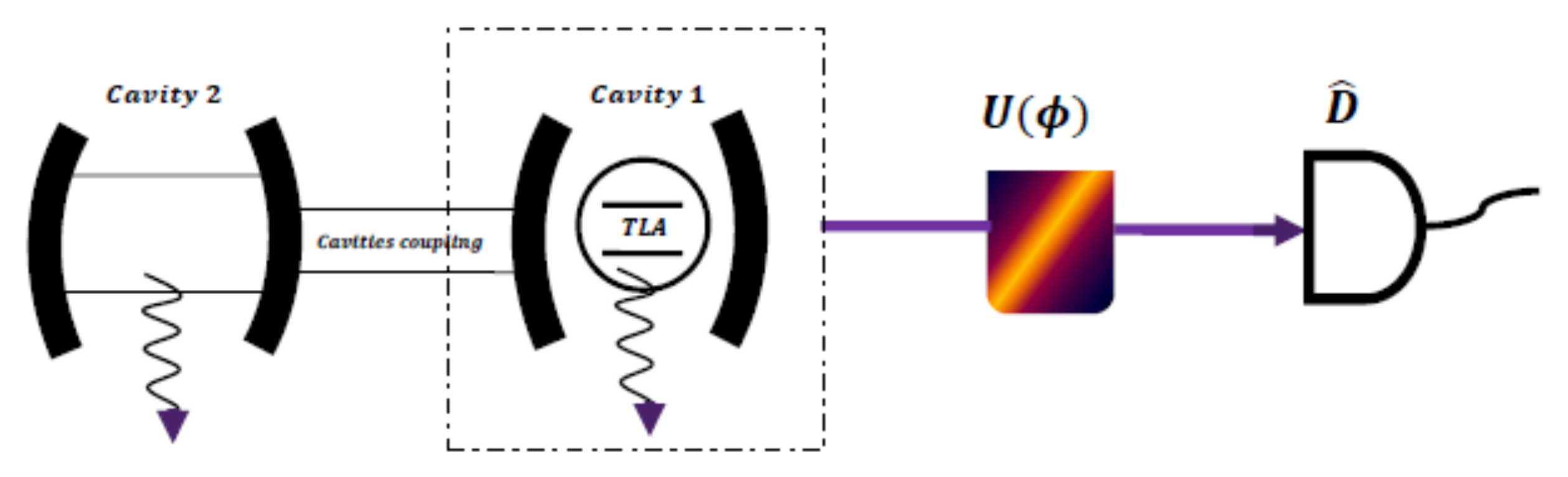
2. Physical Model and Measure of Parameter Estimation

Here is considered a TLA in a cavity 1, which interacts with another cavity 2. The system Hamiltonian can be formulated as
H = ω 0 2 σ Z + i = 1 , 2 ω i A i A i + γ A 1 σ + + A 1 σ + λ A 1 A 2 + A 1 A 2 ,
where ω 0 denotes the transition frequency of the TLA and the operators σ Z and σ ± are defined as σ + = | U L | , σ = | L U | and σ Z = | U U | | L L | , with | L and | U representing the ground and excited states of the TLA, respectively. A i and A i define the cavity field-creation and -annihilation operator, respectively, with the frequency ω i and ω 1 = ω 2 = ω . The function γ describes the TLA–cavity field 1 coupling constant and λ represents the cavity–cavity coupling strength constant.
Taking into account the dissipation of the two cavities, the time evolution of the TLA density matrix ζ is governed by the following master equation:
d ζ d t = i [ H , ζ ] i = 1 2 γ i 2 A i A i ζ + ζ A i A i 2 A i ζ A i .
Here, γ 1 and γ 2 define the photon decay rate cavity 1 and 2, respectively. Strong and weak coupling regimes for the TLA-cavity 1 interaction is identified with the conditions γ > γ 1 / 4 and γ γ 1 / 4 , respectively [31,32]. The Lindblad term in Equation (2), expressed as i = 1 2 γ i 2 A i A i ζ + ζ A i A i 2 A i ζ A i , provides a detailed description of the dissipation processes affecting the cavity fields due to photon leakage into their respective environments. Here, the operators A i and A i for the mode of cavity i explicitly tie the dissipation mechanism to the loss of photons from each cavity. This term encapsulates the independent interaction of each cavity with its own environment, resulting in irreversible energy loss from the system. Being rewritten in its standard form, γ i A i ζ A i 1 2 { A i A i , ζ } , highlights two key physical processes: the term A i ζ A i describes the discrete quantum jump associated with photon emission, while the anticommutator { A i A i , ζ } accounts for the continuous decoherence and energy damping of the cavity modes. Although this dissipation directly targets the cavity fields, it exerts an indirect influence on the TLA through its coupling to cavity 1, governed by the interaction Hamiltonian term γ ( A 1 σ + + A 1 σ ) . This indirect effect plays a critical role in the system’s dynamics as it introduces decoherence that can diminish the quantum Fisher information over time, thereby affecting the precision of parameter estimation in the TLA within the framework of open quantum systems.
To derive the time evolution of the reduced density matrix ζ ( t ) for the TLA interacting with a dissipative cavity system, we consider the TLA coupled to cavity 1, which is, in turn, coupled to cavity 2, starting with the initial total density matrix ρ ( 0 ) = ζ ( 0 ) | 00 00 | C 1 C 2 , where ζ ( 0 ) is the TLA initial state and the cavities are in a vacuum. The system dynamics are restricted to the zero- and single-excitation subspaces, so we use an ansatz for the total density matrix, given by
ρ ( t ) = ( 1 λ ( t ) ) | ψ ( t ) ψ ( t ) | + λ ( t ) | L , 0 , 0 L , 0 , 0 | ,
with | ψ ( t ) = a ( t ) | U , 0 , 0 + b ( t ) | L , 1 , 0 + c ( t ) | L , 0 , 1 . Defining the unnormalized state | ψ ¯ ( t ) = 1 λ ( t ) | ψ ( t ) = a ¯ ( t ) | U , 0 , 0 + b ¯ ( t ) | L , 1 , 0 + c ¯ ( t ) | L , 0 , 1 , we express ρ ( t ) = | ψ ¯ ( t ) ψ ¯ ( t ) | + λ ( t ) | L , 0 , 0 L , 0 , 0 | . The Lindblad master equation yields to the coupled equations:
d a ¯ d t = i Δ a ¯ i γ b ¯ ,
d b ¯ d t = i γ a ¯ i λ c ¯ γ 1 2 b ¯ ,
d c ¯ d t = i λ b ¯ γ 2 2 c ¯ ,
where Δ = ω 0 ω is the detuning and γ 1 and γ 2 are decay rates. By evaluating the Hamiltonian commutator [ H , ρ ] for coherent dynamics and applying the Lindblad dissipation terms for cavity photon losses, we project onto the basis states | U , 0 , 0 , | L , 1 , 0 , and | L , 0 , 1 . This process yields the coupled differential Equations (4)–(6), capturing the TLA–cavity interactions, cavity–cavity coupling, and dissipative decay.
Solving these with initial conditions a ¯ ( 0 ) = ζ u u ( 0 ) , b ¯ ( 0 ) = 0 , c ¯ ( 0 ) = 0 via Laplace transforms, we obtain a ˜ ( s ) = ζ u u ( 0 ) α ( s ) β ( s ) , where α ( s ) and β ( s ) are polynomials, and inverse transforming gives a ¯ ( t ) = ζ u u ( 0 ) χ ( t ) with
χ ( t ) = L 1 α ( s ) β ( s ) .
Tracing over the cavities, ζ ( t ) = Tr C 1 C 2 [ ρ ( t ) ] , we find U | ζ ( t ) | U = | a ¯ ( t ) | 2 = ζ u u ( 0 ) | χ ( t ) | 2 , L | ζ ( t ) | L = 1 ζ u u ( 0 ) | χ ( t ) | 2 , and U | ζ ( t ) | L = ζ u l ( 0 ) χ ( t ) , yielding
ζ ( t ) = ζ u u ( 0 ) | χ ( t ) | 2 ζ u l ( 0 ) χ ( t ) ζ l u ( 0 ) χ * ( t ) 1 ζ u u ( 0 ) | χ ( t ) | 2 ,
fully describing the TLA time evolution.

3. Quantum Fisher Information

In this study, we determine the unobservable parameter ϕ by considering a TLA state ζ , coupled to a cavity system, as a probe. The system experiences a unitary transformation U ϕ . This phase estimation approach is widely applicable across fields such as gravitometry and sensing technologies [33]. The quantum FI serves as a fundamental measure of precision in P-E within quantum mechanics. It quantifies the maximum amount of information that can be extracted about an unknown parameter (denoted as ϕ in our study) from a quantum state, such as the density matrix ζ ( ϕ ) of the TLA interacting with the cavity system. Interestingly, we contextualize quantum FI within our specific model, where a TLA is immersed in a cavity (cavity 1) that interacts with another cavity (cavity 2). We emphasize how QFI enables us to assess the sensitivity of the TLA state to P-E.
An observable ϕ ^ is referred to as the estimator when used to estimate the value of parameter ϕ , provided that the quantum system is in a state of the set { ζ ϕ } . That is, the estimator’s expectation should satisfy Tr ζ ϕ ϕ ^ = ϕ . The quantum FI related to the quantum Cramér–Rao (QC-R) inequality allows us to estimate the accuracy of an unknown parameter. The quantum FI is defined by the formula
Q F = Tr ζ ( ϕ ) D s 2 ,
where ζ ϕ designs the density matrix of the quantum system, ϕ represents the parameter that to be measured, and D s defines the symmetric logarithmic derivation, verifying
2 ζ ( ϕ ) ϕ = ζ ( ϕ ) D s + D s ζ ( ϕ ) .
The QC-R inequality is developed, whereby the bound is asymptotically attained by both the classical theory and the maximum likelihood estimator,
Δ ϕ Δ ϕ QC - R = 1 n Q F ,
where Δ ϕ 2 defines the mean square error with n trials. The aforementioned inequality establishes the minimum amount of uncertainty that may be reasonably estimated for the P-E.
We consider quantum FI as a largely accepted way to detect the precision of the P-E for the system of TLA. We have four steps, as indicated in Figure 1. The first one is to prepare the TLA in an optimal state (input state) | Ψ opt = 1 / 2 | L + | U , with maximum value of the quantum FI [28] and estimating the unknown parameter ϕ . Then, a TLA phase gate is achieved to give
U ϕ : = | L L | + e i ϕ | U U | .
The outcome state is obtained by | ψ out = U ϕ | ψ opt . After the unitary operation and before the measurement is performed, the TLA is subject to the cavity noise. The output state ζ out ϕ is finally measured after the decoherence effect for the P-E.
In the case of pure states, quantum FI is given by Q F = 4 Ψ | Ψ | Ψ | Ψ out | 2 for | Ψ = | Ψ out / ϕ . For a mixed outcome state, the quantum FI is given by
Q F = i , j 2 μ i + μ j | μ i | ζ out ( ϕ ) / ϕ | μ j | 2 .
Here, μ i and | μ i represent the eigenvalues and eigenkets of ζ out , respectively.

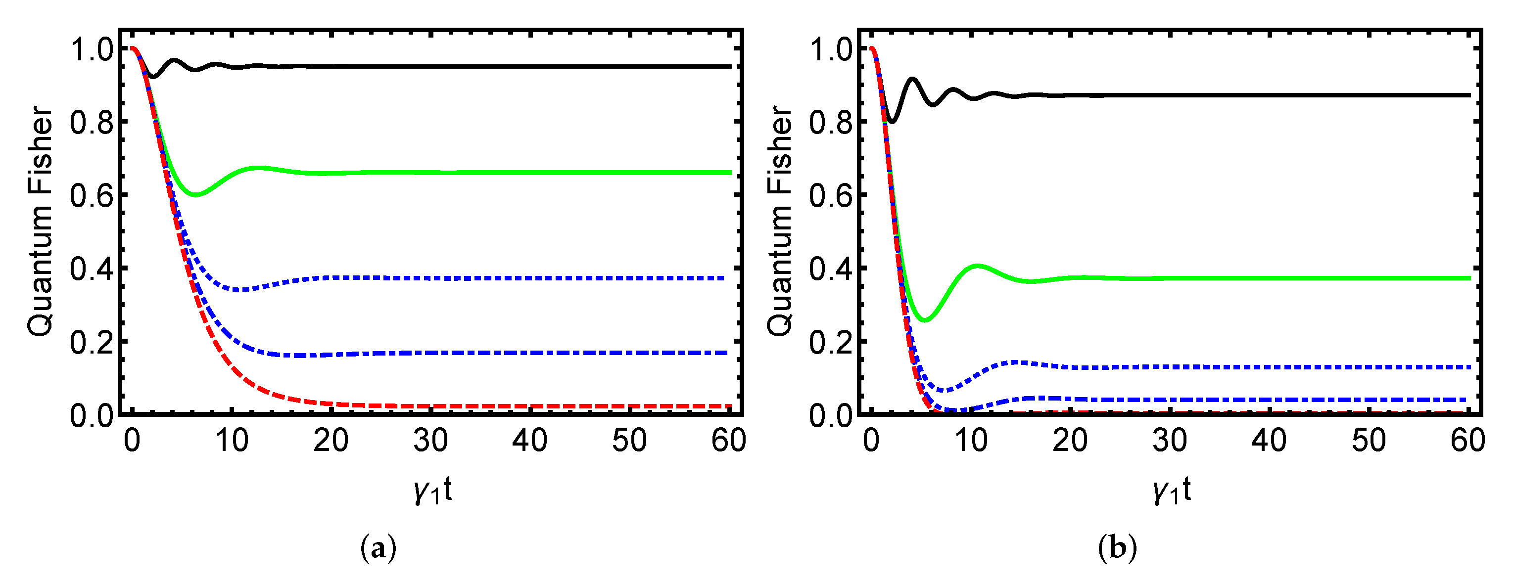
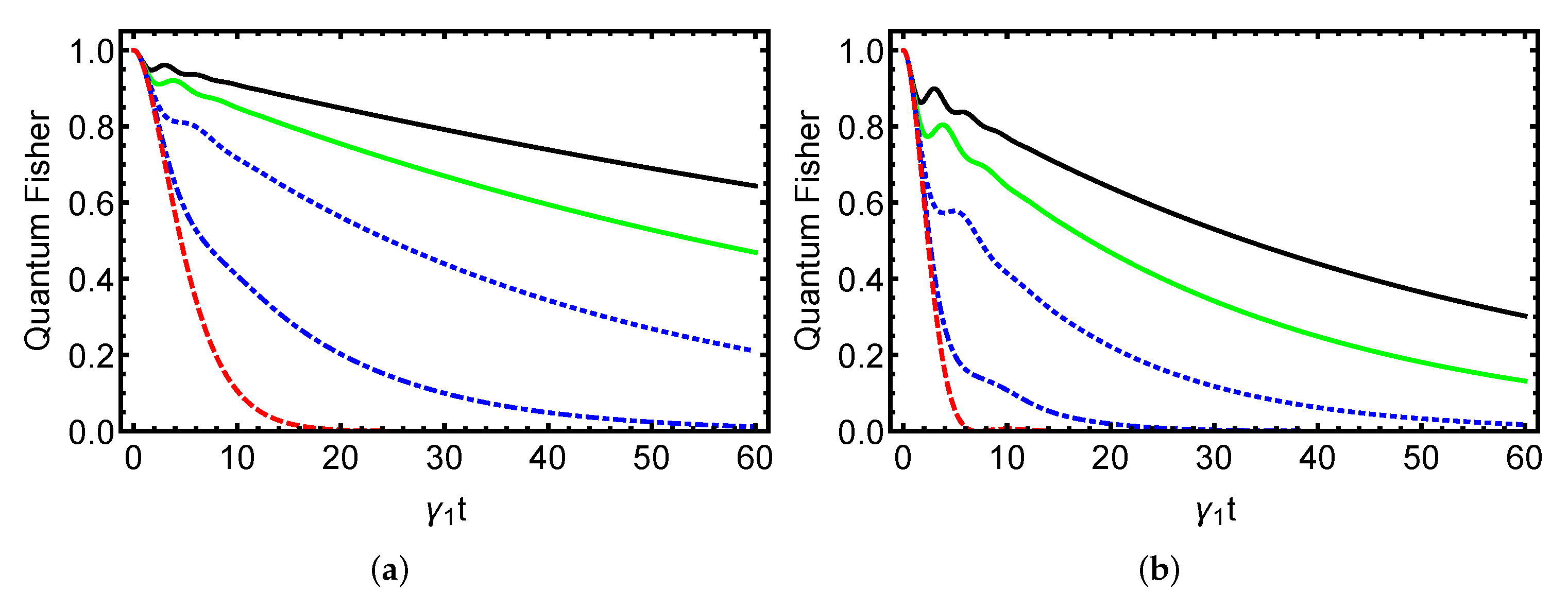
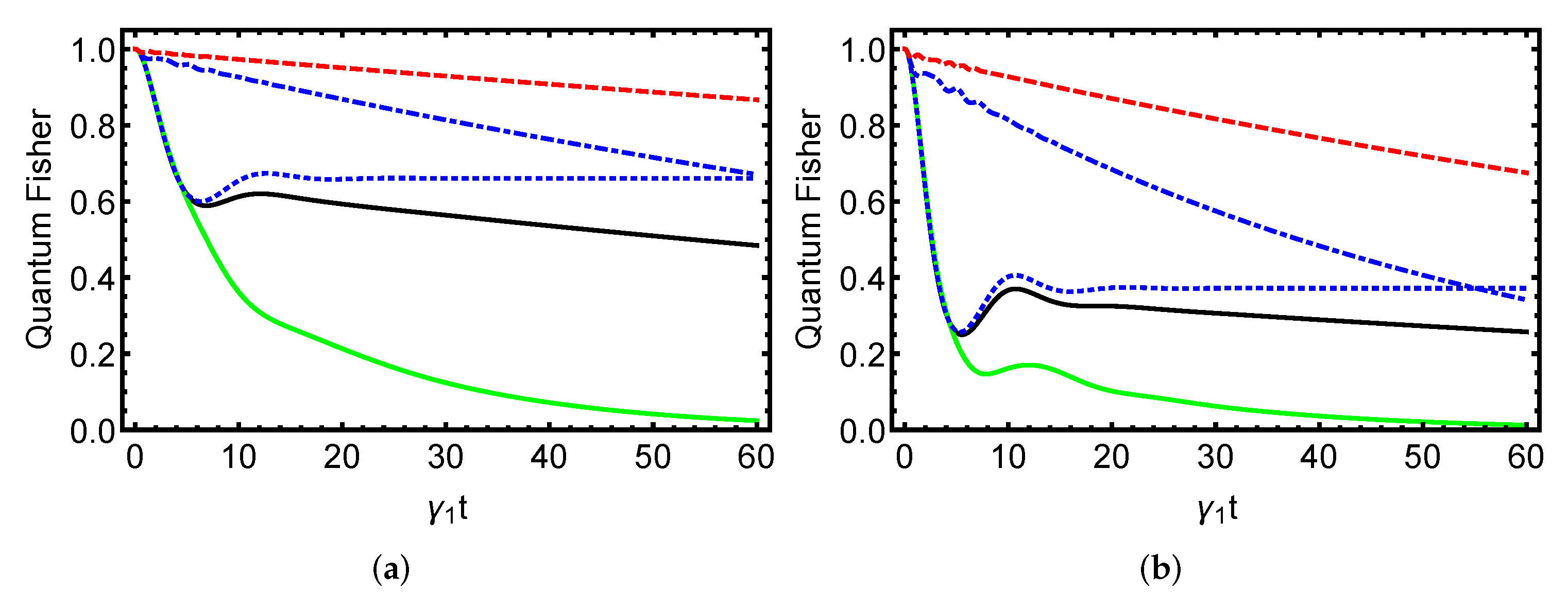
4. Numerical Findings and Discussion

To explore the impact of the cavity 1−cavity 2 interaction and detuning parameter on the precision of the P-E, in Figure 2, Figure 3, Figure 4 and Figure 5, we plot the quantum FI against the time γ 1 t with respect to the quantum model parameters.
Figure 2 displays the dynamics of the quantum FI considering different values of the coupling strength (CS) parameter λ when the TLA is resonant with the cavity 1 ( Δ = 0 ) and that the second cavity 2 is perfect with no photon leakage ( γ 2 = 0 ). In general, we point out that the measure of P-E is strongly affected by the CSs between the cavities during the dynamics. We observe that the FI starts at its maximum value (1) and then exhibits a trapping phenomenon, leading to an asymptotic behavior in the P-E measure. In this regard, we obtain a steady value of measure of P-E that is proportional to the coupling parameter λ . This indicates that the increase in the CS between the cavities results an enhancement in the precision of the P-E. Indeed, we find that employing two coupled cavities enables the preservation of quantum Fisher FI in the long-time limit, achieving stable FI trapping for both weak and strong coupling regimes, across various coupling strengths λ between the two cavities. In Figure 3, we sketch the time variation of FI versus the time γ 1 t for various values of λ in the presence of decay rate γ 2 = 0.5 . We can observe in the result that the amount of quantum FI decays with time and provides oscillations at the beginning of the TLA–cavity interaction as λ becomes large. Moreover, an increase in the CS between the two cavities enhances the quantum FI and delays its decay during the system’s dynamics. In this context, the larger the value of CS is, the higher the precision of the P-E. Interestingly, when examining weak coupling between the TLA and cavity 1 with γ = 0.24 γ 1 , the TLA displays Markovian dynamics, characterized by an asymptotic decline in FI when cavity 2 is absent ( λ = 0 ). Introducing cavity 2 with a sufficiently high coupling strength induces non-Markovian dynamics in the quantum FI, marked by oscillatory behavior. Conversely, in the strong coupling regime between the TLA and cavity 1 ( γ = 0.4 γ 1 ), where FI exhibits collapses and revivals, increasing the coupling parameter λ can shift the TLA’s dynamics from non-Markovian to Markovian and back to non-Markovian. This transition is evidenced by the suppression of oscillations followed by their subsequent re-emergence during the dynamics. Notably, while large λ values can restore non-Markovian dynamics, the resulting oscillatory pattern differs from the initial case λ = 0 , as oscillations appear before the FI fully decays to zero. From these results, the protection and enhancement of the precision of P-E can occur by the optimal control of the CS between the two cavities.
To explore the influence of the detuning, non-resonant TLA–cavity 1 interaction ( Δ 0 ) on the precision of P-E, we display in Figure 4 and Figure 5 the time variation of the measure of FI versus the time γ 1 t , considering various values of Δ with a fixed value of λ . Generally, the measure of FI, which quantifies the amount of information extractable about a parameter from a quantum system, is strongly influenced by the value of the detuning parameter Δ . It can be seen that when the parameter Δ gets close to zero, approaching resonance, the decrease of the quantum FI speeds up during the dynamics. This rapid decline near resonance ( Δ 0 ) arises because the strong coupling between the TLA and cavity 1 amplifies the system’s sensitivity to dissipative effects, accelerating decoherence and thus reducing the FI more quickly. It is important to emphasize that the parameter λ , representing the coupling strength between the TLA and cavity 1, plays an essential role as a benchmark to attain the fastest decrease in the quantum FI with respect to the value of the detuning. In contrast, in the case of large detuning ( Δ λ ), the decrease rate of the amount of FI slows down significantly. This slowdown occurs because large detuning weakens the effective coupling between the TLA and cavity 1, thereby reducing the dissipative influence of the cavity and preserving the system’s quantum coherence, as reflected in the FI’s slower decay. This preservation becomes particularly pronounced when the second cavity in the system is ideal ( γ 2 = 0 ), meaning that it introduces no additional decoherence, allowing the FI and, thus, the precision of parameter estimation to remain stable over longer timescales. In this context, the stationary FI, which would indicate a steady-state level of information, is forbidden out of resonance when the second cavity is perfect. This absence of a stationary FI results in the long-term protection of quantum coherence and, consequently, sustains the precision of the P-E. The interplay between Δ and the ideal second cavity highlights detuning as a powerful control mechanism in open quantum systems, where managing coherence loss is crucial, such as in quantum metrology applications aimed at high-precision measurements. The obtained results demonstrate that the control and protection of FI can be achieved through a judicious choice of Δ and λ , offering a pathway to optimize quantum systems for enhanced parameter estimation under varying environmental interactions.

5. Conclusions

In the present manuscript, we demonstrated the possibility of the control and enhancement of the P-E for a TLA immersed in a cavity field that is in an interaction with other cavity. We analyzed in detail the dynamics of the FI of TLA, considering the influence of the CS of two cavities and the detuning parameter. We showed that for the case of an ideal cavity, a high value of quantum FI can be realized during the dynamics according to the detuning and CS parameters. The results showed that the amount of the quantum FI can be enhanced in a drastic way and protected by regulating the model parameters. In this context, by a convenable choice of the quantum model parameters, long-term protection of the amount of FI can be achieved without it being influenced by the effect of decoherence. The utilization of two cavities can reach this result for an ideal cavity and prove the quantum FI trapping with different SCs for long times. The obtained outcomes offer further guidance for future studies on the regulation of the quantum FI under agreeable circumstances and clarify some empirical observations on the precision of the P-E in the presence of decoherence effects.

Funding

This work was supported and funded by the Deanship of Scientific Research at Imam Mohammad Ibn Saud Islamic University (IMSIU) (grant number IMSIU-DDRSP2503).

Institutional Review Board Statement

Not applicable.

Informed Consent Statement

Not applicable.

Data Availability Statement

Data can be obtained upon reasonable request.

Conflicts of Interest

The authors declare no conflicts of interest.

References

  1. Giovannetti, V.; Lloyd, S.; Maccone, L. Quantum-Enhanced Measurements: Beating the Standard Quantum Limit. Science 2004, 306, 1330. [Google Scholar] [CrossRef] [PubMed]
  2. Dowling, J. Quantum Optical Metrology—The Lowdown On High-N00N States. Contemp. Phys. 2008, 49, 125. [Google Scholar] [CrossRef]
  3. Jones, J.A.; Karlen, S.D.; Fitzsimons, J.; Ardavan, A.; Benjamin, S.C.; Briggs, G.A.D.; Morton, J.J.L. Magnetic Field Sensing Beyond the Standard Quantum Limit Using 10-Spin NOON States. Science 2009, 324, 1166. [Google Scholar] [CrossRef] [PubMed]
  4. Simmons, S.; Jones, J.A.; Karlen, S.D.; Ardavan, A.; Morton, J.J.L. Magnetic field sensors using 13-spin cat states. Phys. Rev. A 2010, 82, 022330. [Google Scholar] [CrossRef]
  5. Higgins, B.L.; Berry, D.W.; Bartlett, S.D.; Wiseman, H.M.; Pryde, G.J. Entanglement-free Heisenberg-limited phase estimation. Nature 2007, 450, 393. [Google Scholar] [CrossRef]
  6. Dorner, U.; Smith, B.J.; Lundeen, J.S.; Wasilewski, W.; Banaszek, K.; Walmsley, I.A. Quantum phase estimation with lossy interferometers. Phys. Rev. A 2009, 80, 013825. [Google Scholar]
  7. Fisher, R.A. Theory of Statistical Estimation. Math. Proc. Camb. Philos. Soc. 1925, 22, 700. [Google Scholar] [CrossRef]
  8. Cramer, H. Mathematical Methods of Statistics; Princeton University Press: Princeton, NJ, USA, 1946. [Google Scholar]
  9. Shukla, R.K.; Chotorlishvili, L.; Mishra, S.K.; Iemini, F. Prethermal Floquet time crystals in chiral multiferroic chains and applications as quantum sensors of AC fields. Phys. Rev. B 2025, 111, 024315. [Google Scholar] [CrossRef]
  10. Kurashvili, P.; Chotorlishvili, L.; Kouzakov, K.A.; Tevzadze, A.G.; Studenikin, A.I. Quantum witness and invasiveness of cosmic neutrino measurements. Phys. Rev. D 2021, 103, 036011. [Google Scholar] [CrossRef]
  11. Haikka, P.; Goold, J.; McEndoo, S.; Plastina, F.; Maniscalco, S. Non-Markovianity, Loschmidt echo, and criticality: A unified picture. Phys. Rev. A 2012, 85, 060101. [Google Scholar] [CrossRef]
  12. Laine, E.-M.; Breuer, H.-P.; Piilo, J.; Li, C.-F.; Guo, G.-C. Nonlocal Memory Effects in the Dynamics of Open Quantum Systems. Phys. Rev. Lett. 2012, 108, 210402. [Google Scholar] [CrossRef]
  13. Mazzola, L.; Rodríguez-Rosario, C.A.; Modi, K.; Paternostro, M. Dynamical role of system-environment correlations in non-Markovian dynamics. Phys. Rev. A 2012, 86, 010102. [Google Scholar] [CrossRef]
  14. Rodríguez-Rosario, C.A.; Modi, K.; Mazzola, L.; Aspuru-Guzik, A. Unification of witnessing initial system-environment correlations and witnessing non-Markovianity. Europhys. Lett. 2012, 99, 20010. [Google Scholar]
  15. Zhang, W.-M.; Lo, P.-Y.; Xiong, H.-N.; Tu, M.W.-Y.; Nori, F. General non-Markovian dynamics of open quantum systems. Phys. Rev. Lett. 2012, 109, 170402. [Google Scholar] [CrossRef] [PubMed]
  16. Apollaro, T.J.G.; Franco, C.D.; Plastina, F.; Paternostro, M. Memory-keeping effects and forgetfulness in the dynamics of a qubit coupled to a spin chain. Phys. Rev. A 2011, 83, 032103. [Google Scholar] [CrossRef]
  17. Žnidarič, M.; Pineda, C.; García-Mata, I. Non-Markovian Behavior of Small and Large Complex Quantum Systems. Phys. Rev. Lett. 2011, 107, 080404. [Google Scholar] [CrossRef] [PubMed]
  18. Breuer, H.-P.; Laine, E.-M.; Piilo, J. Measure for the Degree of Non-Markovian Behavior of Quantum Processes in Open Systems. Phys. Rev. Lett. 2009, 103, 210401. [Google Scholar] [CrossRef]
  19. Laine, E.-M.; Piilo, J.; Breuer, H.-P. Measure for the non-Markovianity of quantum processes. Phys. Rev. A 2010, 81, 062115. [Google Scholar] [CrossRef]
  20. Liu, B.H.; Li, L.; Huang, Y.-F.; Li, C.-F.; Guo, G.-C.; Laine, E.-M.; Breuer, H.-P.; Piilo, J. Experimental control of the transition from Markovian to non-Markovian dynamics of open quantum systems. Nat. Phys. 2011, 7, 931. [Google Scholar] [CrossRef]
  21. Smirne, A.; Mazzola, L.; Paternostro, M.; Vacchini, B. Interaction-induced correlations and non-Markovianity of quantum dynamics. arXiv 2013, arXiv:1302.2055v1. [Google Scholar] [CrossRef]
  22. Lu, X.-M.; Wang, X.; Sun, C.P. Quantum Fisher Information Flow in Non-Markovian Processes of Open Systems. Phys. Rev. A 2010, 82, 042103. [Google Scholar] [CrossRef]
  23. Rajagopal, A.K.; Devi, A.R.U.; Rendell, R.W. Kraus representation of quantum evolution and fidelity as manifestations of Markovian and non-Markovian avataras. Phys. Rev. A 2010, 82, 042107. [Google Scholar] [CrossRef]
  24. Aharonov, D.; Kitaev, A.; Preskill, J. Fault-Tolerant Quantum Computation with Long-Range Correlated Noise. Phys. Rev. Lett. 2006, 96, 050504. [Google Scholar] [CrossRef]
  25. Bellomo, B.; Franco, R.L.; Compagno, G. Non-Markovian Effects on the Dynamics of Entanglement. Phys. Rev. Lett. 2007, 99, 160502. [Google Scholar] [CrossRef]
  26. Zhong, W.; Sun, Z.; Ma, J.; Wang, X.; Nori, F. Fisher information under decoherence in Bloch representation. Phys. Rev. A 2013, 87, 022337. [Google Scholar] [CrossRef]
  27. Ma, J.; Huang, Y.; Wang, X.; Sun, C.P. Quantum Fisher information of the Greenberger-Horne-Zeilinger state in decoherence channels. Phys. Rev. A 2011, 84, 022302. [Google Scholar] [CrossRef]
  28. Sun, Z.; Ma, J.; Lu, X.; Wang, X. Fisher information in a quantum-critical environment. Phys. Rev. A 2010, 82, 022306. [Google Scholar] [CrossRef]
  29. Heng-Na, X.; Xiaoguang, W. Dynamical quantum Fisher information in the Ising model. Phys. A 2011, 390, 4719. [Google Scholar]
  30. Berrada, K. Non-Markovian effect on the precision of parameter estimation. Phys. Rev. A 2013, 88, 035806. [Google Scholar] [CrossRef]
  31. Breuer, H.-P.; Petruccione, F. The Theory of Open Quantum Systems; Oxford University Press: Oxford, NY, USA, 2002. [Google Scholar]
  32. Man, Z.-X.; Xia, Y.-J.; Franco, R.L. Cavity-based architecture to preserve quantum coherence and entanglement. Sci. Rep. 2015, 5, 13843. [Google Scholar] [CrossRef]
  33. Girolami, D.; Tufarelli, T.; Adesso, G. Characterizing Nonclassical Correlations via Local Quantum Uncertainty. Phys. Rev. Lett. 2013, 110, 240402. [Google Scholar] [CrossRef] [PubMed]
Figure 1. Scheme for the P-E in an unitary operation by considering a TLA in cavity 1 that is, in turn, interacted with cavity 2 by cavity coupling λ .
Axioms 14 00368 g001
Figure 2. The quantum FI as a function of time γ 1 t , considering diverse values of the parameter λ for a TLA initially defined in an optimal state | Ψ = 1 / 2 | L + | U with detuning Δ = 0 (TLA is resonant with the cavity 1). | U and | L are the upper and ground states of the TLA, respectively. Label (a) corresponds to γ = 0.24 γ 1 and γ 2 = 0 and label (b) corresponds to γ = 0.4 γ 1 and γ 2 = 0 . The black curve is for λ = 1.5 γ 1 , the green curve is for λ = 0.5 γ 1 , the dotted blue curve is for λ = 0.3 γ 1 , the dot–dash blue curve is for λ = 0.2 γ 1 , and the red curve is for λ = 0.1 γ 1 .
Axioms 14 00368 g002
Figure 3. The quantum FI as a function of time γ 1 t , considering diverse values of the parameter λ for a TLA initially defined in an optimal state | Ψ = 1 / 2 | L + | U with detuning Δ = 0 (TLA is resonant with the cavity 1). | U and | L are the upper and ground states of the TLA, respectively. Label (a) corresponds to γ = 0.24 γ 1 and γ 2 = 0.5 γ 1 and label (b) corresponds to γ = 0.4 γ 1 and γ 2 = 0.5 γ 1 . The black curve is for λ = 2 γ 1 , the green curve is for λ = 1.5 γ 1 , the dotted blue curve is for λ = γ 1 , the dot–dash blue curve is for λ = 0.5 γ 1 , and the red curve is for λ = 0 .
Axioms 14 00368 g003
Figure 4. The quantum FI as a function of time γ 1 t considering diverse values of the detuning parameter Δ for a TLA initially defined in an optimal state | Ψ = 1 / 2 | L + | U with λ = 0.5 γ 1 . | U and | L are the upper and ground states of the TLA, respectively. Label (a) corresponds to γ = 0.24 γ 1 and γ 2 = 0 and label (b) corresponds to γ = 0.4 γ 1 and γ 2 = 0 . The black curve is for Δ = 0.1 γ 1 , the green curve is for Δ = 0.3 γ 1 , the dotted blue curve is for Δ = 0 , the dot–dash blue curve is for Δ = 3 γ 1 and the red curve is for Δ = 5 γ 1 .
Axioms 14 00368 g004
Figure 5. The quantum FI as a function of time γ 1 t , considering diverse values of the detuning parameter Δ for a TLA initially defined in an optimal state | Ψ = 1 / 2 | L + | U with λ = 0.5 γ 1 . | U and | L are the lower and ground states of the TLA, respectively. Label (a) corresponds to γ = 0.24 γ 1 and γ 2 = 0.5 γ 1 and label (b) corresponds to γ = 0.4 γ 1 and γ 2 = 0.5 γ 1 . The black curve is for Δ = 0.1 γ 1 , the green curve is for Δ = 0.3 γ 1 , the dotted blue curve is for Δ = 0 , the dot–dash blue curve is for Δ = 3 γ 1 , and the red curve is for Δ = 5 γ 1 .
Axioms 14 00368 g005
Disclaimer/Publisher’s Note: The statements, opinions and data contained in all publications are solely those of the individual author(s) and contributor(s) and not of MDPI and/or the editor(s). MDPI and/or the editor(s) disclaim responsibility for any injury to people or property resulting from any ideas, methods, instructions or products referred to in the content.

