Abstract
The objective of this manuscript is to investigate the (2+1)-dimensional Chiral nonlinear Schrödinger equation (CNLSE). We employ the traveling wave transformation to convert the nonlinear partial differential equation (NLPDE) into the nonlinear ordinary differential equation (NLODE). Utilizing the two new vital techniques to derive the solitary wave solutions, the generalized Arnous method and the Riccati equation method, we obtained various types of waves like bright solitons, dark solitons, and periodic wave solutions. Sensitivity analysis is also discussed using different initial conditions. Sensitivity analysis refers to the study of how the solutions of the equations respond to changes in the parameters or initial conditions. It involves assessing the impact of variations in these factors on the behavior and properties of the solutions. To better comprehend the physical consequences of these solutions, we showcase them through different visual depictions like 3D, 2D, and contour plots. The findings of this study are original and hold significant value for the future exploration of the equation, offering valuable directions for researchers to deepen knowledge on the subject.
Keywords:
(2 + 1)-dimensional Chiral nonlinear Schrödinger equation; Riccati equation method; generalized Arnous method; sensitivity analysis; solitary wave solutions MSC:
39A1; 39B62; 33B10; 26A48; 26A51
1. Introduction
Real-world phenomena can be best modeled using partial differential equations (PDEs). The nonlinear terms are often seen in PDEs as real-world phenomena that exhibit nonlinear behavior. Nonlinear PDEs are integral to natural sciences such as biology, chemistry, and physics [1,2,3,4]. Furthermore, nonlinear PDEs have applications in emerging fields such as machine learning and microbiology. Conversely, certain complex phenomena can be effectively modeled using nonlinear PDEs. Finding the exact solution of NLPDEs is challenging compared to linear PDEs. There are several techniques to derive solutions for NLPDEs, such as the modified sub-equation method [5], extended -expansion method [6], modified auxiliary equation method [7], Sardar sub-equation method [8], Darboux transformation method [9], Lie symmetry analysis [10], Hirota bilinear method [11], chaotic behavior and bifurcation analysis [12,13,14], and many more methods discussed in [15,16,17].
The nonlinear Schrödinger equation (NLSE) is one of modern science’s most prominent and ubiquitous nonlinear models, appearing in many physics and applied mathematics fields. The most notable solutions of the NLSE are solitary waves, or solitons, which manifest unique properties such as a localized waveform preserved upon interaction with other solitons, giving them a “particle-like” quality. The theory of NLSE solitons was first developed in 1971 by Zakharov and Shabat [18,19]. Following the novel techniques of Gardner et al. [20] and Lax [21,22], Zakharov and Shabat were the first to apply the inverse scattering transform (IST) method to this equation. This method was developed in the quantum scattering theory by Gel’fand et al. [23,24,25,26,27].
In recent decades, NLSE solitons have been experimentally verified across various branches of modern science and identified numerous soliton properties derivable from the IST theory. Hasegawa and Tappert [28] were the first to theoretically demonstrate that an optical pulse in a dielectric fiber forms a solitary wave as the wave envelope obeys the NLSE. The renowned experiment of Mollenauer et al. [29] was explicitly designed to authenticate the use of the prediction. Optical solitons are considered natural data bits and a favorable alternative for the following generation of ultrahigh-speed optical telecommunication systems [30]. Moreover, the theory of picosecond optical solitons, developed within the framework of the NLSE model, has shown remarkable agreement between theory and experiment [31].
In this article, our purpose lies in finding some exact solutions for the following CNLSE [32]
where denotes a complex function, is complex conjugate of , and are the coefficients of nonlinear coupling terms, and stands for the dispersion coefficient. The term is the evolution term. In the literature, several exact solutions of the Chiral stochastic NLSE have been derived using various methods such as the modified Khater and modified Jacobian expansion methods [33], the soliton ansatz method [32], the modified Jacobi elliptic expansion method [34], and the trial solution method [35]. This study aims to find solutions for the considered equation using the generalized Arnous technique and the Reccati equation method [36,37].
The paper provides a comprehensive overview of the proposed model and its analysis. In Section 2, the mathematical analysis of the model is described, wherein Equation (1) is transformed into a nonlinear ordinary differential Equation (ODE) using the traveling wave transformation. Section 3 outlines the methodologies employed, particularly focusing on the generalized Arnous method and its utilization to derive solitary wave solutions for Equation (1). In Section 4, the Riccati, equation method is introduced and applied to Equation (1). Section 5 addresses sensitivity analysis, examining various initial conditions. Finally, the conclusion is presented in Section 6.
2. Description of Proposed Model
Assume that the general form of the (NLPDE) is as follows:
We can convert the NLPDEs into NLODES using the following traveling wave transformation [32,35]
where , , , , , , and are real constants. By inserting Equation (3) into Equation (2), we obtain the NLODE as
Plugging Equation (3) into Equation (1), we obtain the NLODE. The following equations can be derived after transformation from the imaginary and real parts, respectively:
From Equation (5), one may also obtain the following:
The following ODE is deduced from Equation (6):
3. Mathematical Formulation for the Generalized Arnous Method
The main steps of the generalized Arnous (GA) method are given as follows [37]:
Step 1: The GA method provides the solution of Equation (4) as follows:
where and (for ) are constants, and the function satisfies the relation
with
where , , and . Equation (10) has a solution of the form
where A and are random parameters.
Step 2: By matching the nonlinear term with the highest-order derivative term in Equation (4), the value of N for Equation (9) is determined.
Step 3: After substituting Equations (10)–(12) into Equation (3) and , this results in a polynomial of . Next, we collect all terms of the same power and set them equal to zero. Then, by solving the resulting nonlinear algebraic system, the solutions of Equation (2) can be derived.
Solution by Generalized Arnous Method
To find the exact solutions to Equation (8), first, we derive the value of N from Equation (8) by the homogeneous balance principle and then put it into Equation (9); then, Equation (9) can be written as follows:
By putting Equations (9)–(11) into Equation (8), we obtain a polynomial in terms of . This substitution gives a set of equations where all the terms of identical power are collected and set equal to zero as follows:
Solving Equation (14) with the help of Maple, we obtain the following set of solutions:
- Result 1:

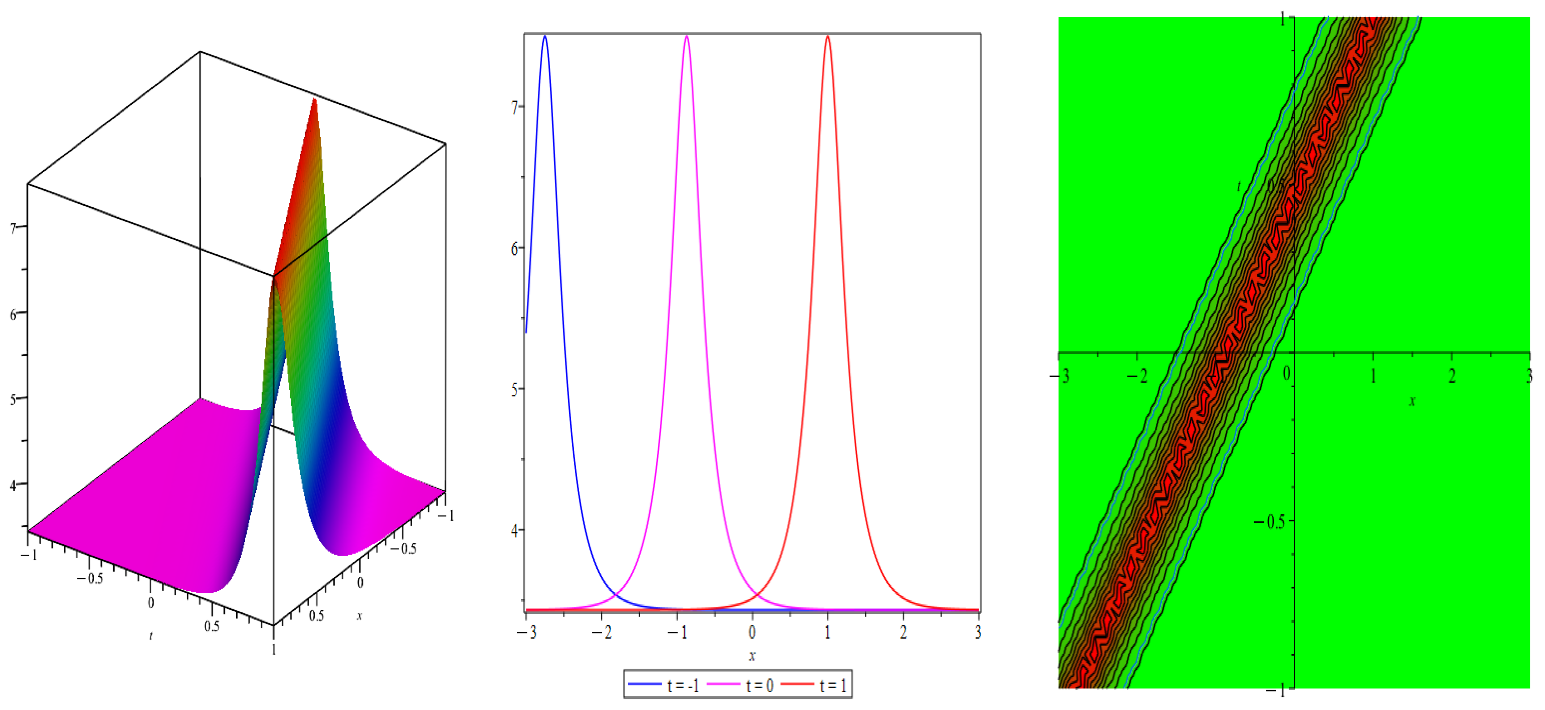
Figure 1.
Graphical representation of solution : , , , , , , and .

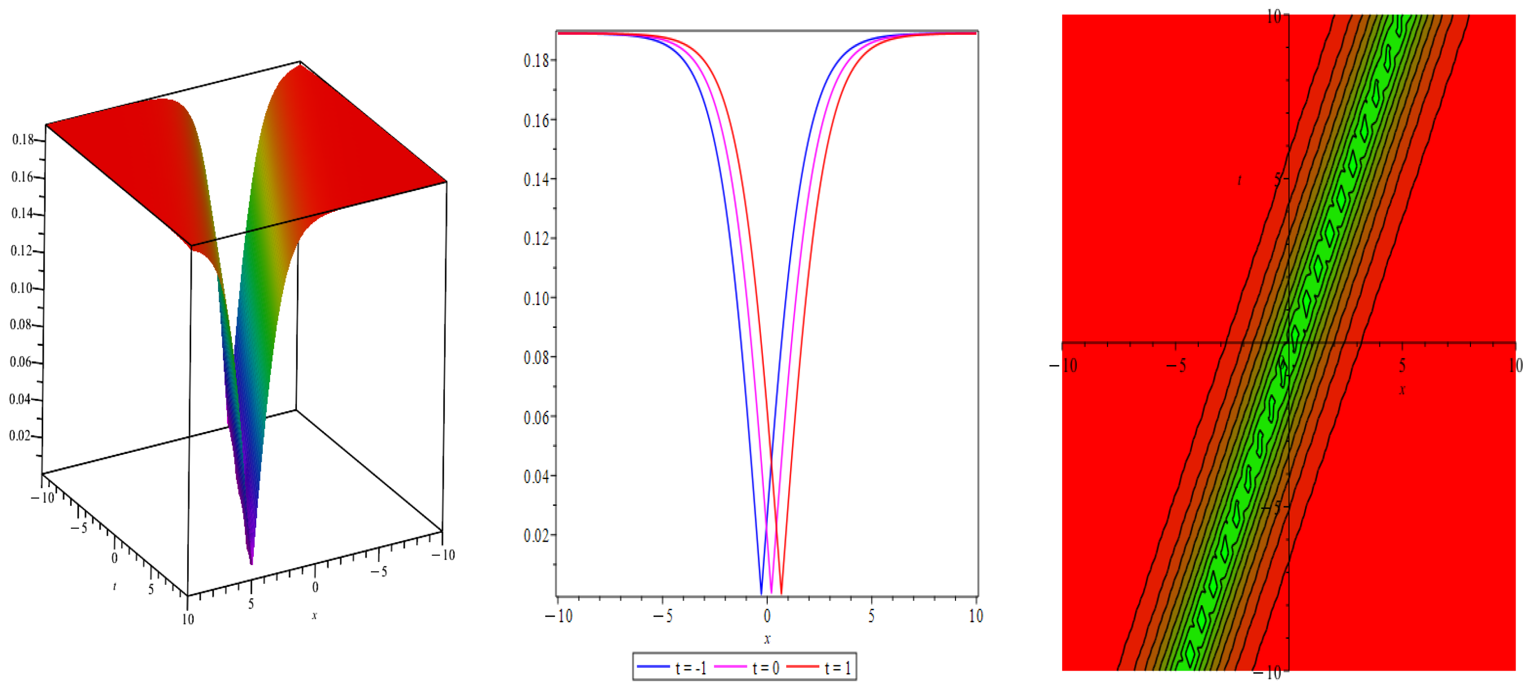
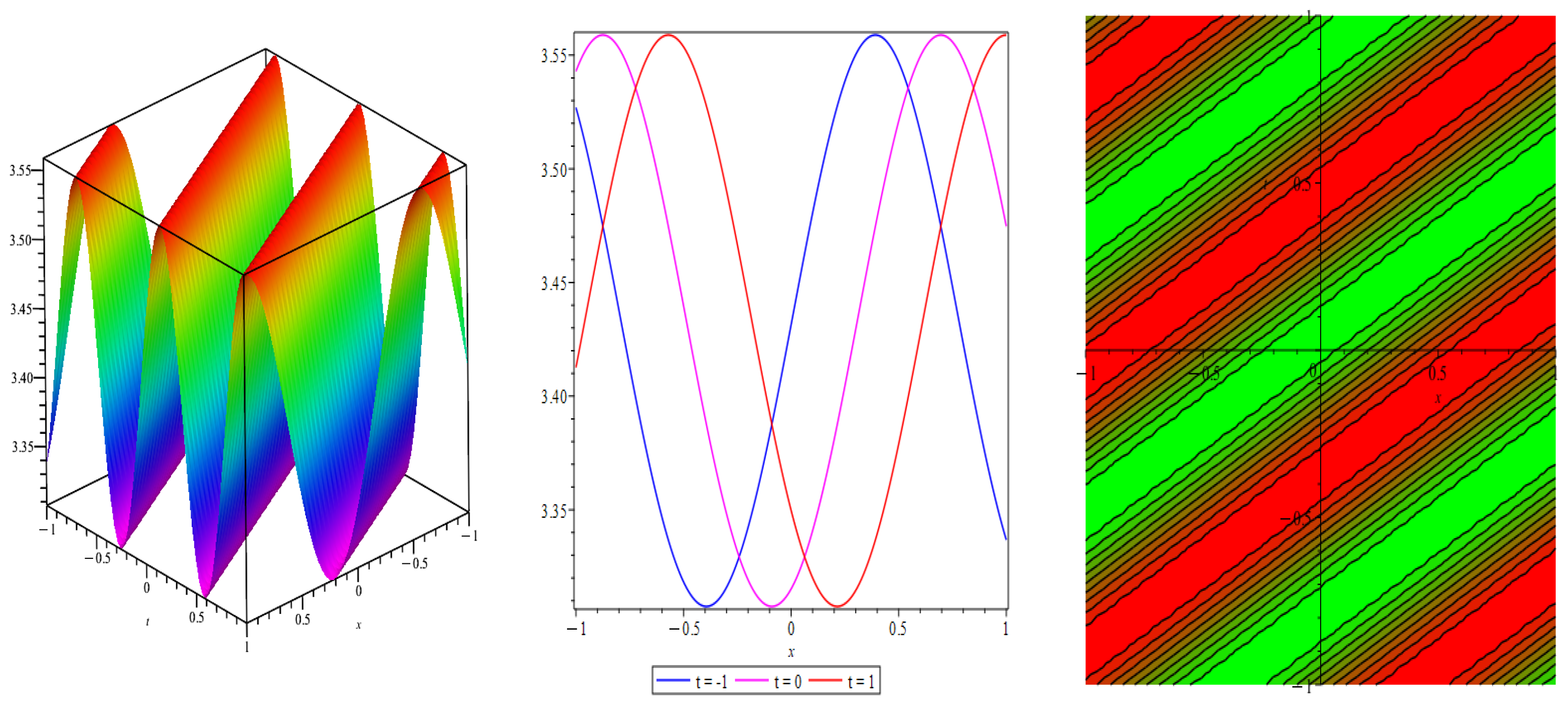
Figure 2.
Graphical representation of solution : , , , , , and .
- Result 2:

Figure 3.
Graphical representation of solution : , , , , , and .
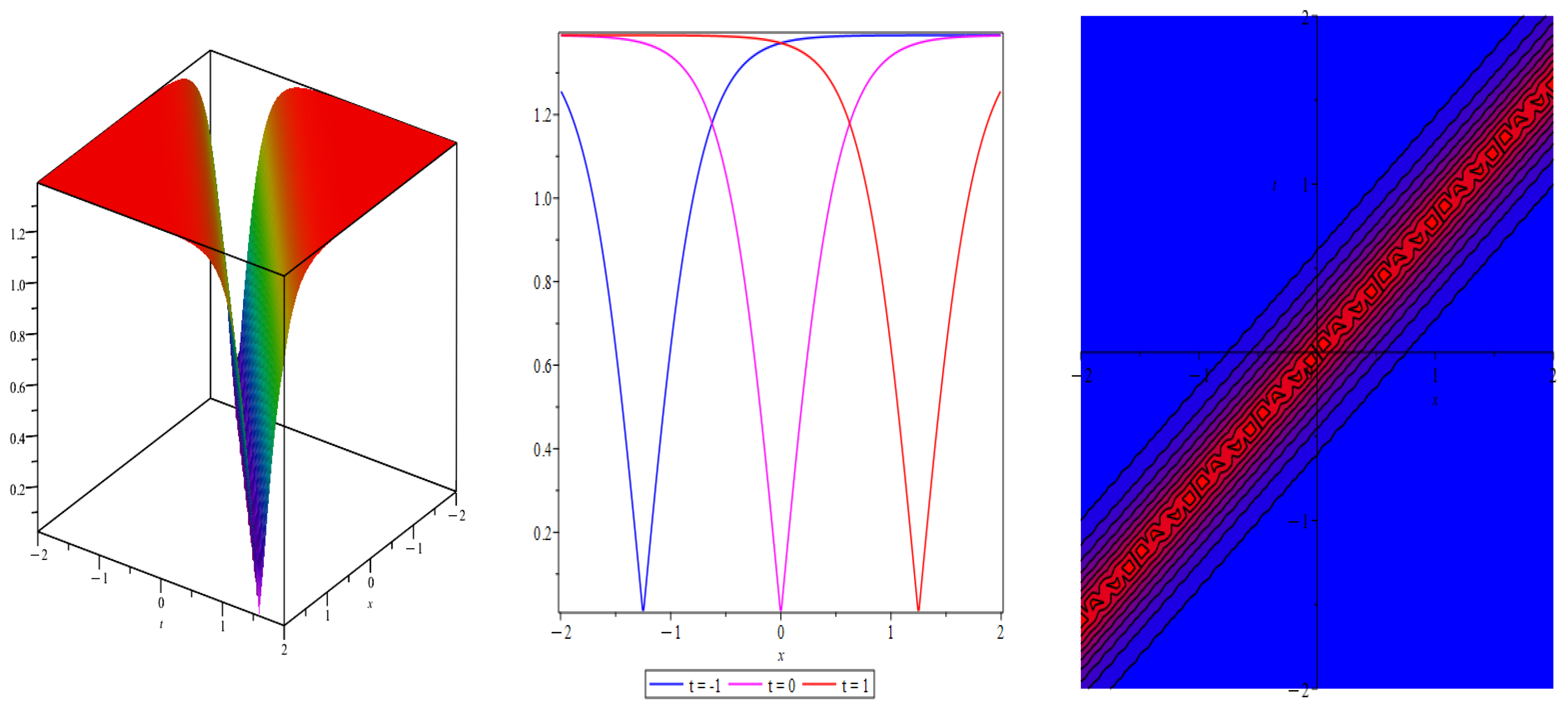
- Result 3:

Figure 4.
Graphical representation of solution : , , , , , and .
4. Riccati Equation Method
We apply the homogeneous balancing principle on Equation (8) and find the value of N. The function holds for the Riccati equation
with the constants , , . The solutions of Equation (28) are
where .
Solution by the Reccati Equation Method
The Reccati equation method indicates the solution of Equation (27) as follows:
Putting Equation (30) into Equation (8) and setting the coefficients of different powers of , we obtain the following set of equations:
The answer to the given set of equations is found by solving them simultaneously.
Corresponding to the above values, we derive the following cases:
- Case 1: When , then we obtain following dark soliton solution (Figure 5)
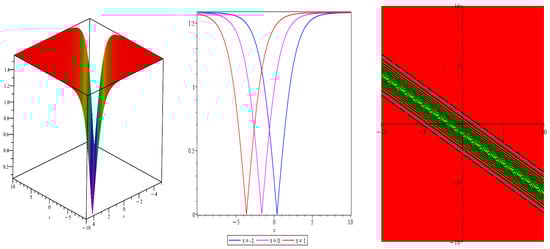 Figure 5. Graphical representation of solution : , , , , , , , and .
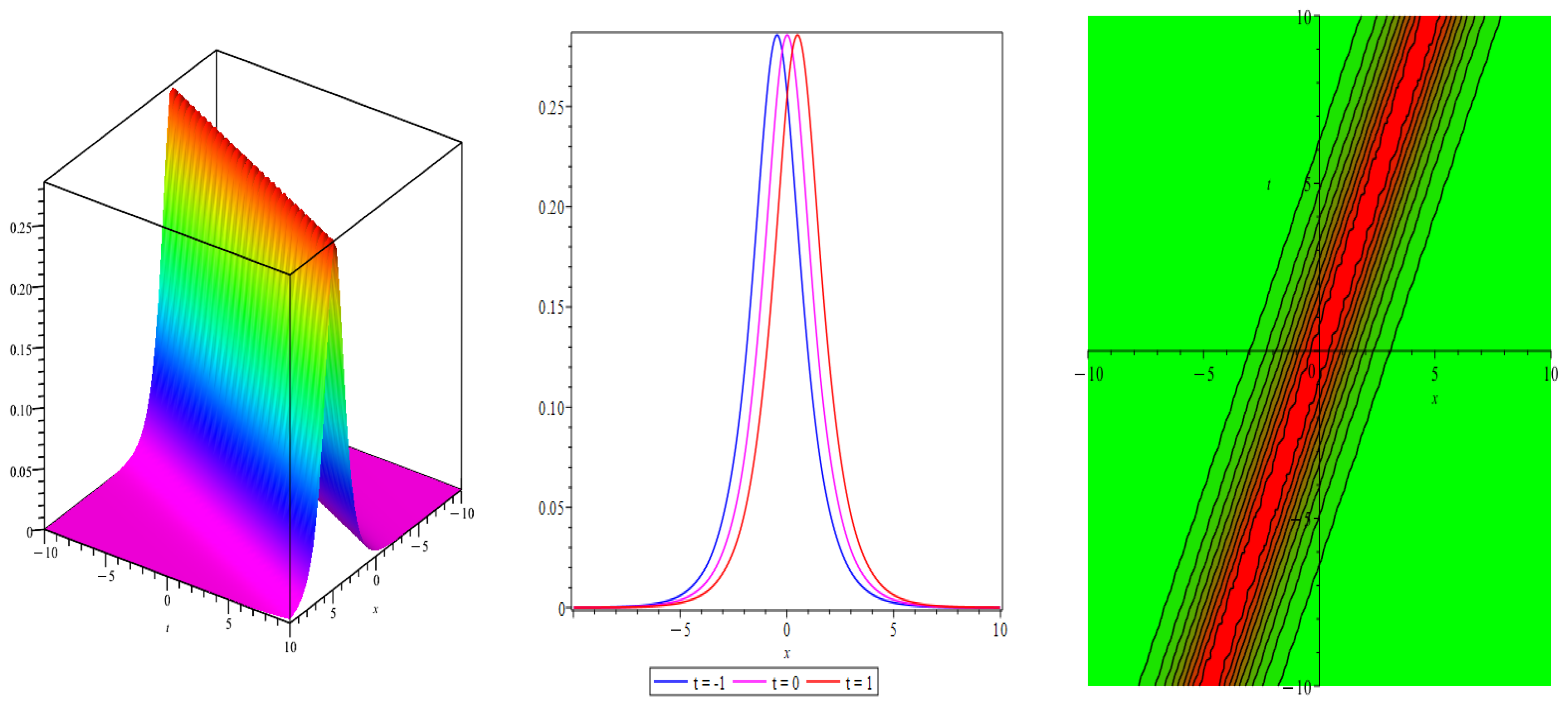
- Case 2: When , then we derive the singular solution as (Figure 6)
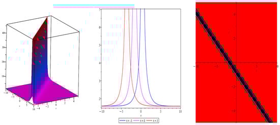 Figure 6. Graphical representation of solution : , , , , , , , and .
- Case 3: When , then we obtain following periodic solution
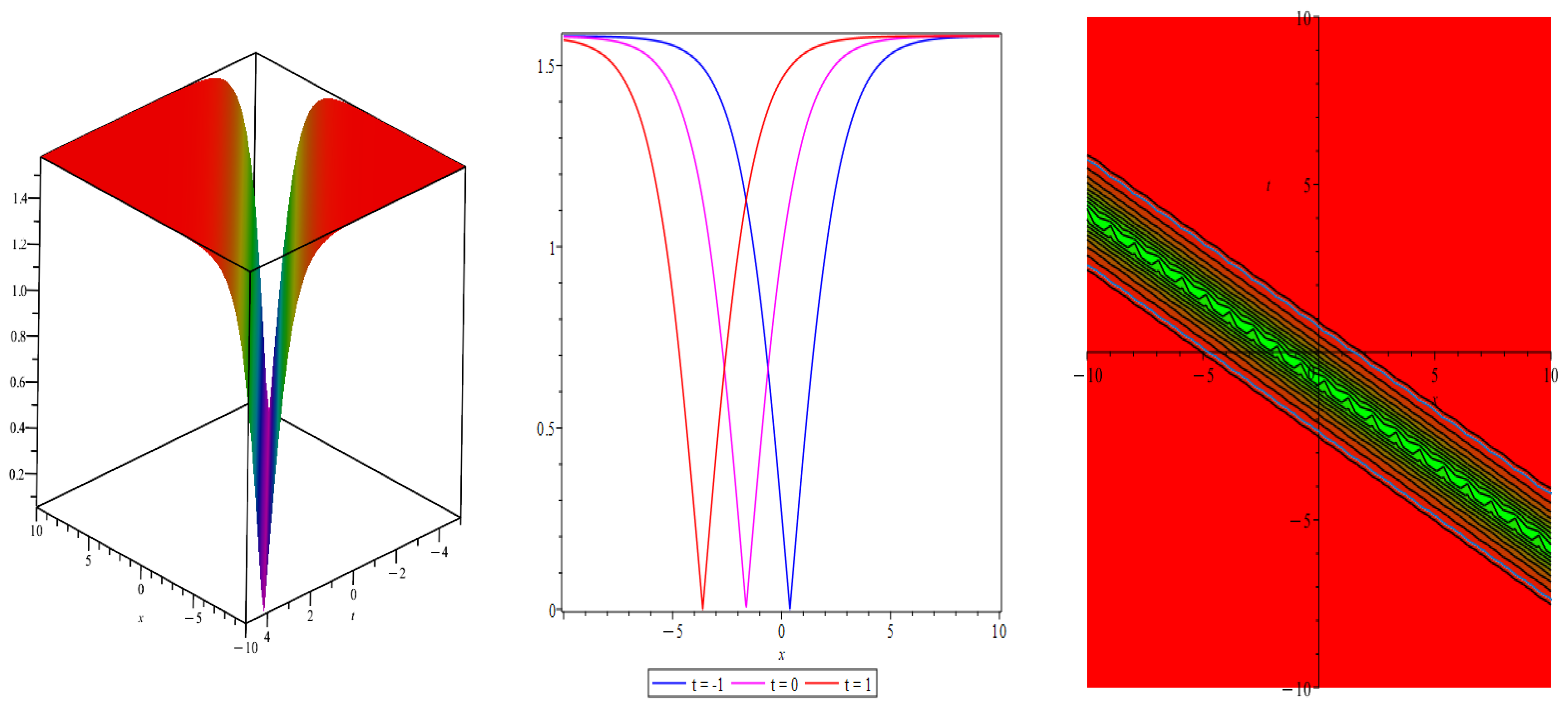
- Case 4: When , then we derive following singular solutions (Figure 7)
 Figure 7. Graphical representation of solution : , , , , , , , and .
- Case 5: When , then we obtain the following solution (Figure 8)
 Figure 8. Graphical representation of solution : , , , , , , , and .
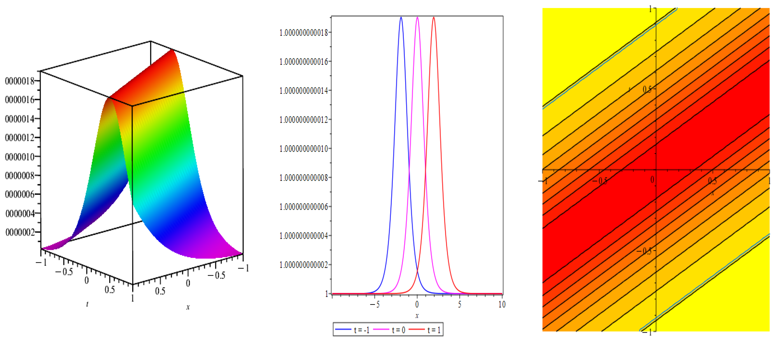
5. Sensitivity Analysis of Equation (1)
This section delves into the sensitivity analysis of the proposed model presented in Equation (8), which is conducted by applying the Runge–Kutta method, leveraging the provided initial conditions. Using the Galilean transformation, Equation (8) can be transformed into two distinct systems of equations. Assuming that , Equation (8) can subsequently be expressed in the following manner [38,39]:
where and .
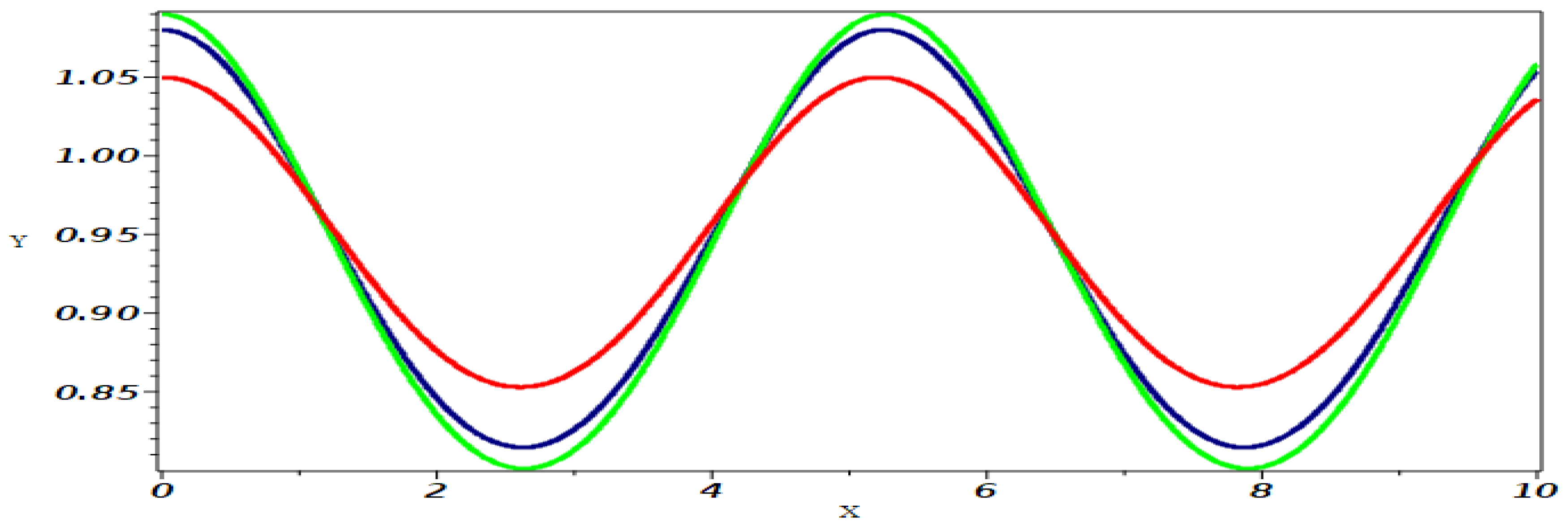
The system Equation (38) is solved using the Runge–Kutta method by applying the suitable parameter values for and . Three solutions, red, navy blue, and green, indicated by , , and , respectively, are shown in Figure 9. Upon observing the figures, it becomes evident that minor alterations in the initial conditions have a negligible impact on the stability of the solution.
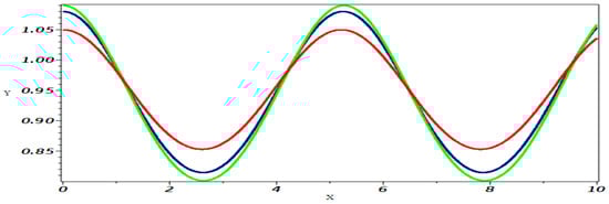
Figure 9.
Sensitivity analysis of system (38) with initial conditions. Three solutions, red, navy blue, and green, indicated by , , and , respectively.
6. Conclusions
In this manuscript, we investigated the (2+1)-dimensional CNLSE, a significant equation in nonlinear wave theory. Using the traveling wave transformation, we successfully converted the NLPDE into a solvable nonlinear ODE. Then, we employed two novel and effective methods as follows: the generalized Arnous method and the Riccati equation method. These methodologies enabled us to extract various solitary wave solutions, encompassing bright solitons, dark solitons, and periodic wave solutions. Each type of solution presents unique characteristics and behaviors that contribute to the broader understanding of wave dynamics governed by the CNLSE. An integral part of our study involved sensitivity analysis, wherein we examined how solutions respond to parameter variations or initial conditions. This analysis is crucial for assessing the robustness and stability of the obtained solutions. By altering different parameters and initial conditions, we observed and analyzed the resultant changes in the behavior and properties of the wave solutions.
To provide a comprehensive understanding of the physical implications of our findings, we visualized the solutions using various graphical representations, including 3D plots, 2D plots, and contour plots. These visualizations not only illustrate the theoretical results but also offer an intuitive grasp of the wave dynamics described by the CNLSE. The outcomes of this study are both original and significant, paving the way for future research endeavors. Our findings offer a solid foundation for the deeper exploration of the CNLSE and its applications in various scientific and engineering fields. This research contributes valuable insights and guidance for researchers aiming to advance the study of nonlinear wave equations and their diverse applications.
Author Contributions
Conceptualization, S.M.; methodology, E.H.; software, E.H. and Y.A.; validation, Y.A.; formal analysis, S.M. and F.S.A.; investigation, S.M.; writing—original draft, E.H.; writing—review & editing, Y.A.; supervision, E.H.; project administration, F.S.A.; funding acquisition, F.S.A. All authors have read and agreed to the published version of the manuscript.
Funding
This work was supported and funded by the Deanship of Scientific Research at Imam Mohammad Ibn Saud Islamic University (IMSIU) (grant number IMSIU-DDRSP2503).
Data Availability Statement
There is no data set to be accessed.
Acknowledgments
The authors thank the Deanship of Scientific Research at Imam Mohammad Ibn Saud Islamic University (IMSIU) for supporting and funding this project.
Conflicts of Interest
The authors declare no conflicts of interest.
References
- Zhou, Q.; Zhu, Q.; Liu, Y.; Yu, H.; Yao, P.; Biswas, A. Thirring optical solitons in birefringent fibers with spatio-temporal dispersion and Kerr law nonlinearity. Laser Phys. 2014, 25, 015402. [Google Scholar] [CrossRef]
- Alquran, M. Physical properties for bidirectional wave solutions to a generalized fifth-order equation with third-order time-dispersion term. Results Phys. 2021, 28, 104577. [Google Scholar] [CrossRef]
- Cinar, M.; Secer, A.; Bayram, M. An application of Genocchi wavelets for solving the fractional Rosenau-Hyman equation. Alex. Eng. J. 2021, 60, 5331–5340. [Google Scholar] [CrossRef]
- Jaradat, I.; Alquran, M. A variety of physical structures to the generalized equal-width equation derived from Wazwaz-Benjamin-Bona-Mahony model. J. Ocean. Eng. Sci. 2022, 7, 244–247. [Google Scholar] [CrossRef]
- Iqbal, M.A.B.; Hussain, E.; Shah, S.A.A.; Li, Z.; Raza, M.Z.; Ragab, A.E.; Az-Zo’bi, E.A.; Ali, M.R. Theoretical examination and simulations of two nonlinear evolution equations along with stability analysis. Results Phys. 2024, 58, 107504. [Google Scholar] [CrossRef]
- Sadaf, M.; Arshed, S.; Akram, G.; Hussain, E. Dynamical behavior of nonlinear cubic-quartic Fokas-Lenells equation with third and fourth order dispersion in optical pulse propagation. Opt. Quantum Electron. 2023, 55, 1207. [Google Scholar] [CrossRef]
- Mahmood, I.; Hussain, E.; Mahmood, A.; Anjum, A.; Shah, S.A.A. Optical soliton propagation in the Benjamin–Bona–Mahoney–Peregrine equation using two analytical schemes. Optik 2023, 287, 171099. [Google Scholar] [CrossRef]
- Cinar, M.; Secer, A.; Ozisik, M.; Bayram, M. Derivation of optical solitons of dimensionless Fokas-Lenells equation with perturbation term using Sardar sub-equation method. Opt. Quantum Electron. 2022, 54, 402. [Google Scholar] [CrossRef]
- Matveev, V.B.; Salle, M.A. Darboux transformations and solitons. In Springer Series in Nonlinear Dynamics; Springer: Berlin/Heidelberg, Germany, 1991. [Google Scholar]
- Malik, S.; Kumar, S.; Biswas, A.; Yıldırım, Y.; Moraru, L.; Moldovanu, S.; Iticescu, C.; Alshehri, H.M. Cubic-quartic optical solitons in fiber bragg gratings with dispersive reflectivity having parabolic law of nonlinear refractive index by Lie symmetry. Symmetry 2022, 14, 2370. [Google Scholar] [CrossRef]
- Hirota, R. The Direct Method in Soliton Theory; Number 155; Cambridge University Press: Cambridge, UK, 2004. [Google Scholar]
- Liu, C.; Li, Z. The dynamical behavior analysis of the fractional perturbed Gerdjikov-Ivanov equation. Results Phys. 2024, 59, 107537. [Google Scholar] [CrossRef]
- Li, Z.; Liu, C. Chaotic pattern and traveling wave solution of the perturbed stochastic nonlinear Schrödinger equation with generalized anti-cubic law nonlinearity and spatio-temporal dispersion. Results Phys. 2024, 56, 107305. [Google Scholar] [CrossRef]
- Li, Z.; Hussain, E. Qualitative analysis and optical solitons for the (1+1)-dimensional Biswas-Milovic equation with parabolic law and nonlocal nonlinearity. Results Phys. 2024, 56, 107304. [Google Scholar] [CrossRef]
- Ablowitz, M.J.; Clarkson, P.A. Solitons, Nonlinear Evolution Equations and Inverse Scattering; Cambridge University Press: Cambridge, UK, 1991; Volume 149. [Google Scholar]
- Ma, W.; Strampp, W. An explicit symmetry constraint for the Lax pairs and the adjoint Lax pairs of AKNS systems. Phys. Lett. A 1994, 185, 277–286. [Google Scholar] [CrossRef]
- Weiss, J.; Tabor, M.; Carnevale, G. The Painlevé property for partial differential equations. J. Math. Phys. 1983, 24, 522–526. [Google Scholar] [CrossRef]
- Shabat, A.; Zakharov, V. Exact theory of two-dimensional self-focusing and one-dimensional self-modulation of waves in nonlinear media. Sov. Phys. JETP 1972, 34, 62. [Google Scholar]
- Zakharov, V.E.; Shabat, A.B. Interaction between solitons in a stable medium. Sov. Phys. JETP 1973, 37, 823–828. [Google Scholar]
- Gardner, C.S.; Greene, J.M.; Kruskal, M.D.; Miura, R.M. Method for solving the Korteweg-deVries equation. Phys. Rev. Lett. 1967, 19, 1095. [Google Scholar] [CrossRef]
- Lax, P.D. Integrals of nonlinear equations of evolution and solitary waves. In Selected Papers Volume I; Springer: Berlin/Heidelberg, Germany, 2005; pp. 366–389. [Google Scholar]
- Ablowitz, M.J.; Kaup, D.J.; Newell, A.C.; Segur, H. Nonlinear-evolution equations of physical significance. Phys. Rev. Lett. 1973, 31, 125. [Google Scholar] [CrossRef]
- Gel’fand, I.M.; Levitan, B.M. On the determination of a differential equation from its spectral function. Izv. Ross. Akad. Nauk. Seriya Mat. 1951, 15, 309–360. [Google Scholar]
- Marchenko, V. Concerning the theory of a differential operator of the second order. Doklady Akad. Nauk SSSR. (NS) 1950, 72, 457–460. [Google Scholar]
- Kay, I.; Moses, H. Reflectionless transmission through dielectrics and scattering potentials. J. Appl. Phys. 1956, 27, 1503–1508. [Google Scholar] [CrossRef]
- Agranovich, Z.; Marchenko, V. The Inverse Problem in the Quantum Theory of Scattering; Izd-vo Khar’kovskogo Universiteta: Kharkov, Ukraine, 1959. [Google Scholar]
- Faddeev, L.D. The inverse problem in the quantum theory of scattering. Uspekhi Mat. Nauk 1959, 14, 57–119. [Google Scholar]
- Hasegawa, A.; Tappert, F. Transmission of stationary nonlinear optical pulses in dispersive dielectric fibers. I. Anomalous dispersion. Appl. Phys. Lett. 1973, 23, 142–144. [Google Scholar] [CrossRef]
- Mollenauer, L.F.; Stolen, R.H.; Gordon, J.P. Experimental observation of picosecond pulse narrowing and solitons in optical fibers. Phys. Rev. Lett. 1980, 45, 1095. [Google Scholar] [CrossRef]
- Banerjee, P.P. Nonlinear Optics: Theory, Numerical Modeling, and Applications; CRC Press: Boca Raton, FL, USA, 2003. [Google Scholar]
- Agrawal, G.P. Nonlinear fiber optics. In Nonlinear Science at the Dawn of the 21st Century; Springer: Berlin/Heidelberg, Germany, 2000; pp. 195–211. [Google Scholar]
- Bulut, H.; Sulaiman, T.A.; Demirdag, B. Dynamics of soliton solutions in the chiral nonlinear Schrödinger equations. Nonlinear Dyn. 2018, 91, 1985–1991. [Google Scholar] [CrossRef]
- Alshahrani, B.; Yakout, H.; Khater, M.M.; Abdel-Aty, A.; Mahmoud, E.E.; Baleanu, D.; Eleuch, H. Accurate novel explicit complex wave solutions of the (2+ 1)-dimensional Chiral nonlinear Schrödinger equation. Results Phys. 2021, 23, 104019. [Google Scholar] [CrossRef]
- Hosseini, K.; Mirzazadeh, M. Soliton and other solutions to the (1+2)-dimensional chiral nonlinear Schrödinger equation. Commun. Theor. Phys. 2020, 72, 125008. [Google Scholar] [CrossRef]
- Eslami, M. Trial solution technique to chiral nonlinear Schrodinger’s equation in (1+2)-dimensions. Nonlinear Dyn. 2016, 85, 813–816. [Google Scholar] [CrossRef]
- Yıldırım, Y.; Biswas, A.; Ekici, M.; Triki, H.; Gonzalez, G.; Alzahrani, A.K.; Belic, M.R. Optical solitons in birefringent fibers for Radhakrishnan–Kundu–Lakshmanan equation with five prolific integration norms. Optik 2020, 208, 164550. [Google Scholar] [CrossRef]
- Bhan, C.; Karwasra, R.; Malik, S.; Kumar, S. Bifurcation, chaotic behavior and soliton solutions to the KP-BBM equation through new Kudryashov and generalized Arnous methods. AIMS Math. 2024, 9, 8749–8767. [Google Scholar] [CrossRef]
- Hussain, E.; Li, Z.; Shah, S.A.A.; Az-Zo’bi, E.A.; Hussien, M. Dynamics study of stability analysis, sensitivity insights and precise soliton solutions of the nonlinear (STO)-Burger equation. Opt. Quantum Electron. 2023, 55, 1274. [Google Scholar] [CrossRef]
- Hussain, E.; Mutlib, A.; Li, Z.; Adham, E.R.; Shah, S.A.A.; Az-Zo’bi, E.A.; Raees, N. Theoretical examination of solitary waves for Sharma–Tasso–Olver Burger equation by stability and sensitivity analysis. Z. Angew. Math. Phys. 2024, 75, 96. [Google Scholar] [CrossRef]

Disclaimer/Publisher’s Note: The statements, opinions and data contained in all publications are solely those of the individual author(s) and contributor(s) and not of MDPI and/or the editor(s). MDPI and/or the editor(s) disclaim responsibility for any injury to people or property resulting from any ideas, methods, instructions or products referred to in the content. |
© 2025 by the authors. Licensee MDPI, Basel, Switzerland. This article is an open access article distributed under the terms and conditions of the Creative Commons Attribution (CC BY) license (https://creativecommons.org/licenses/by/4.0/).