Abstract
This paper proposes a class of randomized Kaczmarz and Gauss–Seidel-type methods for solving the matrix equation , where the matrices A and B may be either full-rank or rank deficient and the system may be consistent or inconsistent. These iterative methods offer high computational efficiency and low memory requirements, as they avoid costly matrix–matrix multiplications. We rigorously establish theoretical convergence guarantees, proving that the generated sequences converge to the minimal Frobenius-norm solution (for consistent systems) or the minimal Frobenius-norm least squares solution (for inconsistent systems). Numerical experiments demonstrate the superiority of these methods over conventional matrix multiplication-based iterative approaches, particularly for high-dimensional problems.
MSC:
65F10; 65F45; 65H10
1. Introduction
The study of matrix equations has emerged as a prominent research topic in numerical linear algebra. In this paper, we investigate the solution of the matrix equation of the form
where , , and . This typical linear matrix equation has attracted considerable attention in both matrix theory and numerical analysis due to its important applications in fields such as systems theory, control theory, image restoration, and more [1,2].
There have been many literature studies and achievements on the matrix equation . For instance, Chu provided sufficient and necessary conditions for the existence of symmetric solutions through singular value decomposition and generalized eigenvalue decomposition [3]. Most of these methods use direct methods, applying generalized inverse, singular value decomposition, QR factorization, and standard correlation decomposition to obtain the necessary and sufficient conditions and analytical expressions for the solution and least squares solution of matrix equations. Due to limitations in computer storage space and computing speed, the direct method may be less efficient in solving large matrices. Therefore, iterative methods for solving linear matrix equations have attracted great interest, such as in [4,5,6,7]. Many methods among these frequently use the matrix multiplication, which consumes a great deal of computing time.
By using the Kronecker products symbol, the matrix equation can be written in the following equivalent matrix vector form:
where the Kronecker product , the right-side vector vec, and the unknown vector vec. With the application of Kronecker products, many algorithms are proposed to solve the matrix Equation (1) (see, e.g., [8,9,10,11,12]). However, when the dimensions of matrices A and B are large, the dimensions of the linear system in Equation (2) increase dramatically, which increases the memory usage and computational cost of numerical algorithms for finding an approximate solution.
Recently, the Kaczmarz method for solving the linear equation has been extended to solve matrix equations. In [13], Shafiei and Hajarian proposed a hierarchical Kaczmarz method for solving the Sylvester matrix equation . Du et al. proposed the randomized block coordinate descent (RBCD) method for solving the matrix least squares problem in [14]. For the consistent matrix equation , Wu et al. proposed the relaxed greedy randomized Kaczmarz (ME-RGRK) and maximal weighted residual Kaczmarz (ME-MWRK) methods [15]. Niu and Zheng proposed two randomized block Kaczmarz algorithms and studied block partitioning techniques [16]. Xing et al. proposed a randomized block Kaczmarz method along with an extended version to solve the matrix equation (consistent or inconsistent) [17]. In [18], Li et al. systematically derived Kaczmarz and coordinate descent algorithms for solving the matrix equations and . Based on this work, we consider the use of Kaczmarz-type methods (row iteration) and Gauss–Seidel methods (column iteration) to solve (1) (which may be consistent or inconsistent) without matrix–matrix production.
The notations used throughout this paper are explained as follows. For a matrix A, its transpose, Moore–Penrose generalized inverse, rank, column space, and Frobenius norm are represented as , , , , and , respectively. We use to denote the inner product of two matrices A and B. Let I denote the identity matrix, where the order is clear from the context. In addition, for a given matrix , we use , , and to denote its ith row, jth column, and smallest nonzero singular value of G, respectively. In addition, we use to denote the expectation and to denote the conditional expectation of the first k iterations, that is,
where and are the row and column indicators selected in the tth step. Let and represent the conditional expectations with respect to the random row index and random column index. Then, it is obvious that .
The rest of this paper is organized as follows. In the next two sections, we discuss the randomized Kaczmarz method for solving the consistent matrix equation and the randomized Gauss–Seidel (coordinate descent) method for solving the inconsistent matrix equation . In Section 4, the extended Kaczmarz method and extended Gauss–Seidel method are derived for finding the minimal F-norm least squares solution of the matrix equation in (1). Section 5 presents some numerical experiments of the proposed methods, then conclusions are provided in the final section. This paper makes several significant advances in solving the matrix equation :
- Algorithm Development: We propose novel randomized Kaczmarz (RK) and Gauss–Seidel-type methods that efficiently handle both full-rank and rank-deficient cases for matrices A and B, addressing both consistent and inconsistent systems.
- Theoretical Guarantees: We rigorously prove that all proposed algorithms converge linearly to either the minimal Frobenius-norm solution (for consistent systems) or the minimal Frobenius-norm least squares solution (for inconsistent systems). We summarize the convergence of the proposed methods in expectation to the minimal F-norm solution for all types of matrix equations in Table 1.
 Table 1. Summary of the convergence of ME-RGRK [15], ME-MWRK [15], RBCD [14], CME-RK (Theorem 1), IME-RGS (Theorem 2), IME-REKRK (Theorem 3), IME-REKRGS (Theorem 4), DREK, and DREGS in expectation to the minimal F-norm solution for all types of matrix equations. (Note: Y means that the algorithm is convergent and N means that it is not.)
 - Computational Efficiency: All proposed methods avoid matrix–matrix multiplications, allowing them to achieve superior performance with low per-iteration cost and minimal storage requirements. Extensive experiments demonstrate the advantages of our approaches over conventional methods, particularly in high-dimensional scenarios.
2. Kaczmarz Method for Consistent Case
If the matrix equation in (1) is consistent, i.e., (necessary and sufficient conditions for consistency; hence, is a solution of the consistent matrix equation in (1)). In particular, if A is full row rank () and B is full column rank (), then the matrix equation in (1) is consistent because is one solution of this equation. In general, the matrix equation in (1) has multiple solutions. Next, we try to find its minimal F-norm solution via the Kaczmarz method.
Assume that A has no row that is all zeros and B has no column that is all zeros. Then, the matrix equation in (1) can be rewritten as the following system of matrix equations:
where . The classical Kaczmarz method, introduced in 1937 [19], is an iterative row projection algorithm for solving a consistent system in which , , and . This method involves only a single equation per iteration, which converges to the least norm solution of with an initial iteration , as follows:
where . If we iterate the system of linear equations , simultaneously and denote , we obtain
where . Then, holds; that is, is the projection of onto the subspace . Thus, we obtain an orthogonal projection method that can be used to solve the matrix equation .
Similarly, we can obtain the following orthogonal column projection method to solve the equation :
where . Then, holds; that is, is the projection of onto the subspace .
If i in (5) and j in (6) are selected randomly with probability proportional to the row norm of A and column norm of B, we obtain a randomized Kaczmarz-type algorithm, which is called the CME-RK algorithm (see Algirithm 1).
| Algorithm 1 RK method for consistent matrix equation (CME-RK) |
|
If the squared row norms of A and squared column norms of B are precomputed in advance, then the cost of each iteration of this method is flops ( for step 5 and for step 6). In the following theorem, we use the idea of the RK method [20] to prove that generated by Algorithm 1 converges to the the minimal F-norm solution of when i and j are selected randomly at each iteration.
Before proving the convergence result of Algorithm 1, we analyze the convergence of and provide the following lemmas, which can be considered as an extension of the theoretical results for solving the linear system of equations in [20]. Let . The sequence is generated by (5) starting from the initial matrix . The following Lemmas 1–3 and their proofs can be found in [18].
Lemma 1
([18]). If the sequence is convergent, it must converge to , provided that .
Lemma 2
([18]). Let be any nonzero matrix. For , it holds that
Lemma 3
([18]). The sequence generated by (5) starting from the initial matrix in which converges linearly to in mean square form. Moreover, the solution error in the expectation for the iteration sequence obeys
where the ith row of A is selected with probability and where .
Similarly, we can obtain the following convergence result of the RK method for the matrix equation .
Lemma 4.
Let . be generated by running a one-step RK update for solving the matrix equation starting from any matrix in which . Then, it holds that
where the jth column of B is selected with probability and where .
Lemma 5.
Let be the subspaces consisting of the solutions to the unperturbed equations and let be the solution spaces of the noisy equations. Then, , where .
Proof.
First, if , then
so .
Next, let . Set ; then,
meaning that . This completes the proof. □
We present the convergence result of Algorithm 1 in the following theorem.
Theorem 1.
The sequence generated by Algorithm 1 starting from the initial matrix converges linearly to the solution of the consistent matrix equation in (1) in mean square form if and . Moreover, the following relationship holds:
where and
Proof.
Let denote the kth iteration of the randomized Kaczmarz method (6) and let be the solution space chosen in the th iteration. Then, is the orthogonal projection of onto . Let denote the orthogonal projection of onto . Using (6) and Lemma 5, we have
Then,
and
Therefore,
By taking the conditional expectation on both side of this equality, we can obtain
Next, we provide the estimates for the first and second parts of the right-hand side of the equality in (9). If , then . It is easy to show that by induction of (6). Then, per Lemma 4, we
For the second part of the right-hand side of (9), we have
Then, applying this recursive relation iteratively and taking the full expectation, we have
If , then
If , then
Setting , (12) then becomes
If , then . Therefore, (12) becomes
This completes the proof. □
Remark 1.
Algorithm 1 has the advantage that and can be iteratively solved alternately at each step; alternatively, the approximate value of can first be obtained iteratively, then the approximate value of can be solved iteratively.
Generally, if we take and , then the initial conditions are all satisfied (, ).
3. Gauss–Seidel Method for Inconsistent Case
If the matrix equation in (1) is inconsistent, then there is no solution to the equation. Considering the least squares solution of the matrix equation in (1), it is obvious that is the unique minimal F-norm least squares solution of the matrix equation in (1), that is,
If A possesses full column rank and B possesses full row rank, then the matrix equation in (1) has a unique least squares solution . In general, the matrix equation in (1) has multiple least squares solutions. Here, we assume that A has no column that is all zeros and B has no row that is all zeros. Next, we find with the Gauss–Seidel (or coordinate descent) method.
When a linear system of equations is inconsistent, i.e., where and (), the RGS (RCD) method [21] below is a very effective method for solving its least squares solution:
where is arbitrary and . Using simultaneous n-iterative formulae for solving , we obtain
where , . This is a column projection method for solving the least squares solution of ; the cost of each iteration in the method is flops if the squared the column norms of A are precomputed in advance.
Similarly, we can solve the least squares solution of using the RGS method:
where , . This is a row projection method; the cost of each iteration of the method is flops if the squared row norms of B are precomputed in advance.
With (14) and (15), we can obtain an RGS method for solving (1) as follows, which is called the IME-RGS algorithm (see Algorithm 2).
| Algorithm 2 RGS method for inconsistent matrix equation (IME-RGS) |
|
In order to prove the convergence of Algorithm 2, we provide the following Lemma 6, the proof of which can be found in [18].
Lemma 6
([18]). Let . The sequence is generated by (14) starting from the initial matrix ; then, the following holds:
where the jth column of A is selected with probability .
Lemma 7.
Let . be generated by running a one-step RGS update for solving the matrix equation starting from any matrix . Then, it holds that
where the ith row of B is selected with probability .
Proof.
From the definition of coordinate descent updates for , we have
which yields . Using the projection formula satisfied by coordinate descent and the properties of MP generalized inversion, we have
Then,
and
Therefore,
By taking the expectation on both sides of (18), we can obtain
The inequality is obtained by Lemma 2 because all columns of are in the range of . This completes the proof. □
Theorem 2.
Let denote the sequence generated by Algorithm 2 for the inconsistent matrix equation in (1) starting from any initial matrix and . In exact arithmetic, it holds that
Proof.
Let denote the kth iteration of the RGS method in (15) that solves and let be the one-step RGS iteration that solves from ; then, we have
Then,
and
Therefore,
By taking the conditional expectation on both sides of (19), we can obtain
The last inequality is obtained by Lemmas 6 and 7. Applying this recursive relation iteratively, we have
where and are defined in Theorem 1. This completes the proof. □
Remark 2.
If A has full column rank and B has full row rank, Theorem 2 implies that converges linearly in expectation to . If A does not have full column rank or B does not have full row rank, Algorithm 2 fails to converge (see Section 3.3 of Ma et al. [22]).
Remark 4.
Remark 5.
In Algorithm 2 and can be iteratively solved alternately at each step, or the approximate value of can be iteratively obtained first and then the approximate value of can be iteratively solved. By using Lemmas 6 and 7, we can obtain similar convergence results. We omit the proof for the sake of conciseness.
4. Extended Kaczmarz Method and Extended Gauss–Seidel Method for
When the matrix equation in (1) is inconsistent and either matrix A or matrix B is not full of rank, we can consider the REK method or REGS method to solve the matrix equation in (1) using the ideas of [23,24,25].
4.1. Inconsistent, A Not Full Rank, and B Full Column Rank ()
The matrix equation is solved by the REK method [23,24], while the matrix equation is solved by the RK method [20], because always has a solution ( is full row rank). For this case, we use the REK-RK method to solve , which is called the IME-REKRK algorithm (see Algorithm 3). The cost of each iteration of this method is flops ( for step 6, for step 7, and for step 8) if the squared row and column norms of A and the squared column norms of B are precomputed in advance.
| Algorithm 3 REK-RK method for inconsistent matrix equation (IME-REKRK) |
|
Lemma 8.
Let and ; then, it holds that
Proof.
Because and , we have
This completes the proof. □
Similar to the proof of Lemma 3, we can prove the following Lemma 9.
Lemma 9.
Let , and let denote the kth iterate of RK applied to with the initial guess . If , then converges linearly to in mean square form. Moreover, the solution error in expectation for the iteration sequence obeys
where the jth column of A is selected with probability .
Lemma 10.
The sequence is generated by the REK method for starting from the initial matrix , in which and the initial guess is with . In exact arithmetic, it holds that
where the ith row of A is selected with probability and the jth column of A is selected with probability .
Proof.
Let denote the kth iteration of the REK method for and let be the one-step Kaczmarz update for the matrix equation from , i.e.,
We have
and
It follows from
and
that
By taking the conditional expectation on the both sides of this equality, we have
Next, we provide the estimates for the two parts of the right-hand side of (24). It follows from
that
By and , , we have . Then, by , it is easy to show that and by induction. It follows from
that
This completes the proof. □
With these preparations, the convergence proof of Algorithm 3 is provided below.
Theorem 3.
Let denote the sequence generated by Algorithm 3 (B is full column rank) with the initial guess in which . The sequence is generated by the REK method for starting from the initial matrix , in which and with . In exact arithmetic, it holds that
where
Proof.
Similar to the proof of Theorem 1 using Lemma 10 and Lemma 4, we can obtain
If , then from the analytical properties of geometric series we can obtain
If , then
If , then
Substituting the above inequalities into (27) completes the proof. □
4.2. Inconsistent, A Not Full Rank, and B Full Row Rank ()
The matrix equation is solved by the REK method, while the matrix equation is solved by the RGS method, because has a unique least-squares solution ( is full column rank). For this case, we refer the algorithm for solving as IME-REKRGS (see Algorithm 4). The cost of each iteration of this method is flops ( for step 6, for step 7, and for step 8) if the squared row and column norms of A and the squared row norms of B are precomputed in advance.
| Algorithm 4 REK-RGS method for inconsistent matrix equation (IME-REKRGS) |
|
Similarly, letting , we can transform the equation into the system of equations composed of
The matrix equation is solved by the RGS method because it has a unique least squares solution ( is full column rank), while the matrix equation is solved by the REK method. For this case, we refer the algorithm for solving as IME-RGSREK.
The above two methods can be seen as the combination of two separate algorithms; thus, we do not discuss the algorithms in detail. We only provide the convergence results of the IME-REKRGS method, and omit the proof.
Theorem 4.
Let denote the sequence generated by IME-REKRGS method (B is full row rank) with initial guess . The sequence is generated by the REK method for starting from the initial matrix , in which and the initial guess is with . In exact arithmetic, it holds that
4.3. Double Extended Kaczmarz Method for Solving General Matrix Equation
In general, the matrix equation in (1) may be inconsistent, and A and B may not be full rank; thus, we consider solving both matrix equations and by the REK method. The algorithm is described below (see Algorithm 5).
| Algorithm 5 Double REK method for general (DREK) |
|
The convergence result is the superposition of the corresponding convergence results of the two REK methods, and the proof is omitted.
Similar to the DREK method, we can employ the double REGS (DREGS) method to solve the general matrix equation (see Algorithm 6). Because the convergence results and proof methods are very similar to the previous ones, we omit them here.
| Algorithm 6 Double REGS method for general (DREGS) |
|
5. Numerical Experiments
In this section, we present some experimental results of the proposed algorithms for solving various matrix equations and compare them with ME-RGRK and ME-MWRK from [15] for consistent matrix equations and RBCD from [14] for inconsistent matrix equations. All experiments were carried out in MATLAB (version R2020a) on a DESKTOP-8CBRR86 with an Intel(R) Core(TM) i7-4712MQ CPU@2.30GHz, 8GB RAM, and Windows 10.
All computations were started from the initial guess and terminated when the relative error (RE) of the solution, defined by
at the the current iteration , satisfied or exceeded the maximum iteration K = 50,000, where . We report the average number of iterations (denoted as “IT”) and average computing time in seconds (denoted as“CPU”) for 20 repeated trial runs of the corresponding method. We considered the following methods:
- CME-RK (Algorithm 1) compared with ME-RGRK and ME-MWRK in [15] for consistent matrix equations. We used in the ME-RGRK method, which is the same as in [15].
- IME-RGS (Algorithm 2), IME-REKRGS (Algorithm 4) compared with RBCD in [14] for inconsistent matrix equations. We used in the RBCD method, which is the same as in [14].
- IME-REKRK (Algorithm 3), DREK (Algorithm 5), and DREGS (Algorithm 6) for inconsistent matrix equations. The last two methods have no requirements regarding whether matrix A and matrix B have full row rank or full column rank.
We tested the performance of various methods with synthetic dense data and real-world sparse data. Synthetic data were generated as follows:
- Type I: For given , the entries of A and B were generated from a standard normal distribution, i.e., We also constructed the rank-deficient matrix by or , etc.
- Type II: As in [16], for given , and , we constructed a matrix A by , where and are orthogonal columns matrices, is a diagonal matrix with the first diagonal entries uniformly distributed numbers in , and the last two diagonal entries are . Similarly, for given , and , we constructed a matrix B by , where and are orthogonal columns matrices, is a diagonal matrix with the first diagonal entries uniformly distributed numbers in , and the last two diagonal entries are .
The real-world sparse data were taken from the Florida sparse matrix collection [26]. Table 2 lists the features of these sparse matrices.
Table 2.
Detailed features of the sparse matrices from [26].
5.1. Consistent Matrix Equation
First, we compared the performance of the ME-RGRK, ME-MWRK, and CME-RK methods for the consistent matrix equation . To construct a consistent matrix equation, we set , where is a random matrix generated by .
Example 1.
The ME-RGRK, ME-MWRK, and CME-RK methods with synthetic dense data.
Table 3 and Table 4 report the average IT and CPU of ME-RGRK, ME-MWRK, and CME-RK for solving a consistent matrix with Type I and Type II matrices. In the following tables, the item “>” indicates that the number of iteration steps exceeded the maximum iterations (50,000), while the item “-” indicates that the method did not converge. From Table 3, it can be seen that the CME-RK method vastly outperforms the ME-RGRK and ME-MWRK methods in terms of both IT and CPU times. The CME-RK method has the least iteration steps and runs for the least time regardless of whether or not matrices A and B are full column/row rank. We observe that when the linear system is consistent, the speed-up is at least 2.00 and the largest speed-up reaches 3.75. As the matrix dimension increases, the CPU time of the CME-RK method increases only slowly, while the running times of ME-RGRK and ME-MWRK increase dramatically. The numerical advantages of CME-RK for large consistent matrix equations are more obvious in Table 4. Moreover, when and are large (e.g., ), the convergence speeds of ME-RGRK and ME-MWRK are very slow, which is because the convergence rate of these two methods depends on .
Table 3.
IT and CPU of ME-RGRK, ME-MWRK, and CME-RK for consistent matrix equations with Type I.
Table 4.
IT and CPU of ME-RGRK, ME-MWRK and CME-RK for consistent matrix equations with Type II.
Figure 1 shows the plots of the relative error (RE) in base-10 logarithm versus the IT and CPU of different methods with Type I (, ) and Type II (, ). Again, it can be seen that the relative error of CME-RK decreases rapidly with the increase in iteration steps and the computing time.
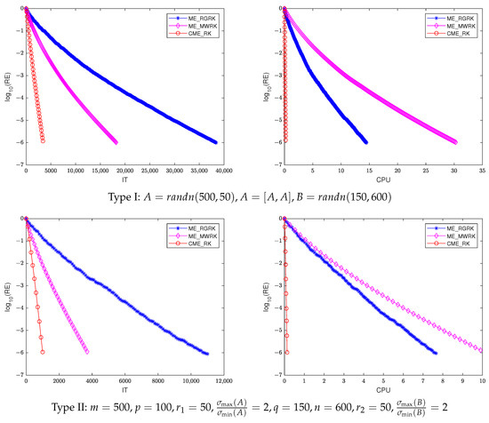
Figure 1.
IT (left) and CPU (right) of different methods for consistent matrix equations with Type I (top) and Type II (bottom).
Example 2.
The ME-RGRK, ME-MWRK, and CME-RK methods with real-world sparse data.
For the sparse matrices from [26], the numbers of iteration steps and the computing times for the ME-RGRK, ME-MWRK, and CME-RK methods are listed in Table 5. It can be observed that the CME-RK method successfully computes an approximate solution of the consistent matrix equation for various A and B. For the fist three cases in Table 5, the ME-RGRK, ME-MWRK, and CME-RK methods all converge to the solution; however, the CME-RK method is significantly better than the ME-RGRK and ME-MWRK methods in terms of both iteration steps and running time. For the last three cases, the ME-RGRK and ME-MWRK methods fail to converge to the solution because the iteration steps exceed the maximum of 50,000.
Table 5.
IT and CPU of ME-RGRK, ME-MWRK, and CME-RK for the consistent matrix equations with sparse matrices from [26], where T represents transposition.
5.2. Inconsistent Matrix Equation
Next, we compare the performance of the RBCD, IME-RGS, and IME-REKRGS methods for the inconsistent matrix equation , where B is full row rank. To construct an inconsistent matrix equation, we set , where and R are random matrices generated by and . In addition, we show the experiment results of the REKRK, DREK, and DREGS methods, which do not require B to have full row rank.
Example 3.
The RBCD, IME-RGS, and IME-REKRGS methods with synthetic dense data.
Table 6 and Table 7 report the average IT and CPU of the RBCD, IME-RGS, and IME-REKRGS methods for solving an inconsistent matrix with Type I and Type II matrices. Figure 2 shows the plots of the relative error (RE) in base-10 logarithm versus the IT and CPU of different methods with Type I () and Type II (). From these tables, it can be seen that the IME-RGS and IME-REKRGS methods are better than the RBCD method in terms of IT and CPU time, especially when the matrix dimension is large (see the last two cases in Table 6) or when is large (see the last three cases in Table 7). From Figure 2, it can be seen that the IME-RGS and IME-REKRGS methods converge faster than the RBCD method, although the relative error of RBCD decreases faster in the initial iteration.
Table 6.
IT and CPU of RBCD, IME-RGS, and IME-REKRGS for inconsistent matrix equations with Type I.
Table 7.
IT and CPU of RBCD, IME-RGS, and IME-REKRGS for inconsistent matrix equations with Type II.
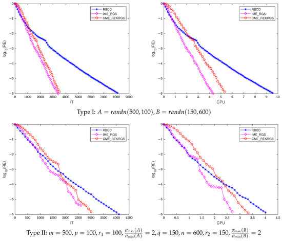
Figure 2.
IT (left) and CPU (right) of different methods for inconsistent matrix equations with Type I (top) and Type II (bottom).
Example 4.
The RBCD, IME-RGS, and IME-REKRGS methods with real-world sparse data.
Table 8 lists the average IT and CPU of the RBCD, IME-RGS, and IME-REKRGS methods for solving an inconsistent matrix with sparse matrices. It can be observed that the IME-RGS and IME-REKRGS methods require less CPU time than the RBCD method in all case and less IT in all cases except for .
Table 8.
IT and CPU of RBCD, IME-RGS, and IME-REKRGS for inconsistent matrix equations with sparse matrices from [26].
Example 5.
The IME-REKRK, DREK, and DREGS methods.
Finally, we tested the effectiveness of the IME-REKRK, DREK, and DREGS methods for inconsistent matrix equations, including both synthetic dense data and real-world sparse data. The features of A and B are provided in Table 9, while the experimental results are listed in Table 10. For the DREK and DREGS methods, the iteration steps and running time for calculating and are represented by “+”. From Table 10, it can be observed that the IME-REKRK method ia able to compute an approximate solution to the linear least squares problems when B has full column rank. The DREK and DREGS methods can successfully solve the linear least squares solution for all cases.
Table 9.
Detailed features of A and B for Example 5.
Table 10.
IT and CPU of the IME-REKRK, DREK, and DREGS methods for the inconsistent matrix equations.
6. Conclusions
In this paper, we propose a Kaczmarz-type algorithm for the consistent matrix equation . We develop a Gauss–Seidel-type algorithm to address the inconsistent case when A is full column rank and B is full row rank. In addition, we introduce extended Kaczmarz and extended Gauss–Seidel algorithms for inconsistent systems where either A or B lacks full rank. Theoretical analyses establish the linear convergence of these methods to the unique minimal Frobenius-norm solution or the least squares solution (i.e., ). Numerical experiments demonstrate the efficiency and robustness of the proposed algorithms.
In future work, we aim to extend the proposed algorithms to tensor equations and more general multilinear systems as well as to further explore their use in large-scale optimization and machine learning applications. Additionally, we will investigate accelerated variants of the proposed algorithms to enhance their convergence rates by incorporating strategies such as greedy selection rules, block iterative processing, and adaptive step size techniques. These improvements are expected to significantly boost computational efficiency, making the proposed methods more suitable for high-dimensional and real-world problems.
Author Contributions
Conceptualization, W.Z. and L.X.; methodology, L.X.and W.B.; validation, W.Z. and W.B.; writing—original draft preparation, W.Z.; writing—review and editing, L.X. and W.L.; software, W.Z. and L.X.; visualization, W.Z. and L.X. All authors have read and agreed to the published version of the manuscript.
Funding
This research received no external funding.
Institutional Review Board Statement
The authors declare that they have no known competing financial interests or personal relationships that could have appeared to influence the work reported in this paper.
Data Availability Statement
The datasets that support the findings of this study are available from the corresponding author upon reasonable request.
Acknowledgments
The authors are thankful to the referees for their constructive comments and valuable suggestions, which have greatly improved the original manuscript of this paper.
Conflicts of Interest
The authors declare no conflicts of interest.
References
- Bouhamidi, A.; Jbilou, K. A note on the numerical approximate solutions for generalized Sylvester matrix equations with applications. Appl. Math. Comput. 2008, 206, 687–694. [Google Scholar] [CrossRef]
- Zhou, B.; Duan, G. On the generalized Sylvester mapping and matrix equations. Syst. Control Lett. 2008, 57, 200–208. [Google Scholar] [CrossRef]
- Chu, K. Symmetric solutions of linear matrix equations by matrix decompositions. Linear Algebra Appl. 1989, 119, 35–50. [Google Scholar] [CrossRef]
- Ding, F.; Chen, T.W. Iterative least-squares solutions of coupled sylvester matrix equations. Syst. Control Lett. 2005, 54, 95–107. [Google Scholar] [CrossRef]
- Ding, F.; Liu, P.; Ding, J. Iterative solutions of the generalized Sylvester matrix equations by using the hierarchical identification principle. Appl. Math. Comput. 2008, 197, 41–50. [Google Scholar] [CrossRef]
- Wang, X.; Li, Y.; Dai, L. On Hermitian and skew-Hermitian splitting iteration methods for the linear matrix equation AXB = C. Comput. Math. Appl. 2013, 65, 657–664. [Google Scholar] [CrossRef]
- Tian, Z.; Tian, M.; Liu, Z.; Xu, T. The Jacobi and Gauss-Seidel-type iteration methods for the matrix equation AXB = C. Appl. Math. Comput. 2017, 292, 63–75. [Google Scholar] [CrossRef]
- Fausett, D.; Fulton, C. Large least squaress problems involving Kronecker products. SIAM J. Matrix Anal. Appl. 1994, 15, 219–227. [Google Scholar] [CrossRef]
- Zha, H. Comments on large least squaress problems involving Kronecker products. SIAM J. Matrix Anal. Appl. 1995, 16, 1172. [Google Scholar] [CrossRef]
- Zhang, F.; Li, Y.; Guo, W.; Zhao, J. Least squares solutions with special structure to the linear matrix equation AXB = C. Appl. Math. Comput. 2011, 217, 10049–10057. [Google Scholar] [CrossRef]
- Cvetkovic, D. Re-nnd solutions of the matrix equation AXB = C. J. Aust. Math. Soc. 2008, 84, 63–72. [Google Scholar] [CrossRef]
- Peng, Z. A matrix LSQR iterative method to solve matrix equation AXB = C. Int. J. Comput. Math. 2010, 87, 1820–1830. [Google Scholar] [CrossRef]
- Shafiei, S.; Hajarian, M. Developing Kaczmarz method for solving Sylvester matrix equations. J. Frankl. Inst. 2022, 359, 8991–9005. [Google Scholar] [CrossRef]
- Du, K.; Ruan, C.; Sun, X. On the convergence of a randomized block coordinate descent algorithm for a matrix least squaress problem. Appl. Math. Lett. 2022, 124, 107689. [Google Scholar] [CrossRef]
- Wu, N.; Liu, C.; Zuo, Q. On the Kaczmarz methods based on relaxed greedy selection for solving matrix equation AXB = C. J. Comput. Appl. Math. 2022, 413, 114374. [Google Scholar] [CrossRef]
- Niu, Y.; Zheng, B. On global randomized block Kaczmarz algorithm for solving large-scale matrix equations. arXiv 2022, arXiv:2204.13920. [Google Scholar]
- Xing, L.; Bao, W.; Li, W. On the convergence of the randomized block Kaczmarz algorithm for solving a matrix equation. Mathematics 2023, 11, 4554. [Google Scholar] [CrossRef]
- Li, W.; Bao, W.; Xing, L. Kaczmarz-type methods for solving matrix equations. Int. J. Comput. Math. 2024, 101, 708–731. [Google Scholar] [CrossRef]
- Kaczmarz, S. Angenherte auflsung von systemen linearer gleichungen. Bull. Internat. Acad. Polon. Sci. Lett. A 1937, 32, 335–357. [Google Scholar]
- Strohmer, T.; Vershynin, R. A randomized Kaczmarz algorithm with exponential convergence. J. Fourier Anal. Appl. 2009, 15, 262–278. [Google Scholar] [CrossRef]
- Leventhal, D.; Lewis, A. Randomized methods for linear constraints: Convergence rates and conditioning. Math. Oper. Res. 2010, 35, 641–654. [Google Scholar] [CrossRef]
- Needell, D. Randomized Kaczmarz solver for noisy linear systems. BIT Numer. Math. 2010, 50, 395–403. [Google Scholar] [CrossRef]
- Zouzias, A.; Freris, N. Randomized extended Kaczmarz for solving least squares. SIAM J. Matrix Anal. Appl. 2013, 34, 773–793. [Google Scholar] [CrossRef]
- Du, K. Tight upper bounds for the convergence of the randomized extended Kaczmarz and Gauss-Seidel algorithms. Numer. Linear Algebra Appl. 2019, 26, e2233. [Google Scholar] [CrossRef]
- Ma, A.; Needell, D.; Ramdas, A. Convergence properties of the randomized extended Gauss-Seidel and Kaczmarz methods. SIAM J. Matrix Anal. Appl. 2015, 36, 1590–1604. [Google Scholar] [CrossRef]
- Davis, T.; Hu, Y. The University of Florida sparse matrix collection. ACM Trans. Math. Softw. 2011, 38, 1–25. [Google Scholar] [CrossRef]
Disclaimer/Publisher’s Note: The statements, opinions and data contained in all publications are solely those of the individual author(s) and contributor(s) and not of MDPI and/or the editor(s). MDPI and/or the editor(s) disclaim responsibility for any injury to people or property resulting from any ideas, methods, instructions or products referred to in the content. |
© 2025 by the authors. Licensee MDPI, Basel, Switzerland. This article is an open access article distributed under the terms and conditions of the Creative Commons Attribution (CC BY) license (https://creativecommons.org/licenses/by/4.0/).