Article

Influence of Heat Transfer on Stress Components in Metallic Plates Weakened by Multi-Curved Holes

by
Faizah M. Alharbi
* and
Nafeesa G. Alhendi
Mathematics Department, Faculty of Sciences, Umm Al-Qura University, Makkah 24227, Saudi Arabia
*
Author to whom correspondence should be addressed.
Axioms 2025, 14(5), 369; https://doi.org/10.3390/axioms14050369
Submission received: 9 January 2025 / Revised: 1 April 2025 / Accepted: 23 April 2025 / Published: 14 May 2025
(This article belongs to the Special Issue Mathematical Methods in the Applied Sciences, 2nd Edition)

Abstract

:
This manuscript addresses an application study by employing a mathematical model of a thermoelastic plate weakened by multi-curved holes under the effect of stress forces in the presence of heat conduction. When the initial heat flow is directed to the plate system, complex variable procedures are used to compute the basic Goursat functions, taking into account the time-dependent variables through conformal mapping, which transfers the domain to the exterior of a unit circle. The problem reduces to a general form of a contact problem in two dimensions, which is called an integrodifferential equation of the second type with the Cauchy kernel. Additionally, different hole shapes are generated using Maple 2023. Computational simulations are performed to determine the normal and shear stress components in the presence and absence of heat effects at various times. Furthermore, numerical calculations of Goursat functions are carried out and graphically displayed for some specific materials. This investigation provides valuable information about industries, such as those regarding ceramic tile, glass, rubber, paint, ceramic pigment, and metal alloys.

1. Introduction

Thermoelasticity covers a broad spectrum of phenomena. It covers the theories of heat conduction, strain, and stress induced by heat flow when the temperature and strain fields are combined. Thermoelasticity allows us to identify the stresses created by a temperature field, as well as the temperature distribution caused by the actions of internal forces that change over time; see [1]. When external loads are applied to the plate’s structural components, the stress tends to concentrate in the area around the holes. Each component of the stress tensor is governed by a Poisson-type differential equation, and the boundary conditions and differential equations pertaining to the plane problem of thermoelectricity in stresses are examined; see [2]. Manickam et al. [3] attempted to use curvilinear fibers in a thermal setting to examine the nonlinear thermoelastic buckling characteristics of composite variable stiffness beams with several layers. Yuan et al. [4] used the method of fundamental solutions to study the stress fields of anti-plane finite elastic materials with holes that were susceptible to traction or displacement boundaries. An analytical solution for an elastic infinite plate with ellipse and circle holes that experiences internal traction along the holes as well as uniform stresses and shears at infinity was presented by Lu et al. [5]. For anisotropic elastic media with polygonal holes with rounded corners, Hsieh et al. [6] used the perturbation method with conformal mapping and the nonconformal mapping scheme to obtain two sets of solutions of Green’s functions. Savruk [7] undertook a survey of the findings from studies on the concentrations of stresses in elastic bodies that are weakened by nonsmoothly contoured notches and curvilinear holes. Using the Stroh formalism, Hsieh [8] derived a comprehensive solution for an infinite anisotropic plate featuring a hole deviating from an elliptical shape, which is subjected to uniform loading at infinity. Guo and Lu [9] presented a novel means of resolving the elastic–plastic fields along the major-axis line of the elliptical hole using the complex variable method. Boundary problems for infinite plates with holes have been covered by a number of authors [10,11]. Some of them used the Laurent theorem to show that the responses were power series. Applying Goursat functions is another method for handling complex variables. They integrate the characteristics of the circle or any mapped area of Cauchy integrals outside of a unit circle by using the general rational mapping function z = c Ω ( ξ ) . Two complex functions are the result of their solution. Abdou et al. [11] used a limitless plate with two curved holes to deduce the first and second types using the Goursat functions in the complex variable technique. In order to tackle the basic issues of an infinite plate with a hole that is weakened by a strong pole of any kind, Abdou and Monaquel [12] used the Cauchy singular approach. The exterior conformal mapping of the inclusion provided Mattei and Lim [13] with a coordinate system, which they used to build a density basis function. Using the complex variable technique, Alhazmi et al. [14] considered an infinite elastic plate featuring two holes that compromise its integrity, aiming to develop a closed form of Goursat functions with varying time. Based on rational approximations for solving Dirichlet problems and least-squares fitting on the boundary, Trefethen [15] created novel techniques for numerical conformal mapping. Under certain conditions, Alharbi and Alhendi [16] used particular conformal mapping to represent the stress distributions of a thin endlessly flexible plate affected by many curvilinear apertures. A complex integrodifferential equation in the right half-plane was solved by Jann [17] using an infinite plate that was weakened by a curvilinear hole.
In this paper, we consider the conformal mapping
z = Ω ( ξ ) = A + j = 1 M m j ξ j , | A | > 0 , 0 m j A < 1 j ,
where j = 1 , 2 , , M ;   A = A 1 + i A 2 , | A | > 0 , m j = m j 1 + m j 2 , z = Ω ( ξ ) , ξ = ρ e i θ = ς + i η mapped the domain of the plate that maps the curvilinear hole into the domain outside the unit circle | ξ | > 1 , and m j A is a parameter constrained in such a way that it Ω ( ξ ) does not approach zero or reach infinity beyond the unit circle. The two complex analytic potential functions, Goursat functions χ ( ξ , τ ) and ϖ ( ξ , τ ) , at variable times are derived. Transferring the complex plane, which contains curvilinear holes, is the method’s concept. We employ a particular conformal mapping to achieve this. A method to easily look into shapes from the conformal map is shown, along with a way to compute the conformal map for the chosen bounds. By employing the complex variable technique with the Cauchy methodology, we solve the boundary value problem and obtain a closed version of the Goursat functions. We then simplify the problem using the second-type integrodifferential equation with a Cauchy kernel. We also identify the components of normal and shear stress. After explaining the different physical applications, we calculate and visualize the normal and shear stress components for each at the specified values using the Maple 2023 program. Finally, we discuss the main results of the work.

2. Formulation of the Problem

Take into consideration a thin infinite elastic plate with a thickness of h and weakened by closed and indefinite shape holes C; see Figure 1.
Equation (1) is used to conformally transfer the points inside the holes to the unit circle.
Let q represent the constant temperature gradient, and let Θ = q y denote the heat equation that flows uniformly in the negative direction of the y-axis. The equation Θ = Θ ( x , y ) posits that the temperature increase Θ is uniform throughout the thickness of the plate.
The following is satisfied by the heat equation in this case since C distributes the heat uniformly
2 Θ = 0 , 2 = 2 x 2 + 2 y 2 = 2 r 2 + 1 r r + 1 r 2 2 θ 2 , Θ r = 0 , on the boundary r = r o .
The following formula can be used to express the thermoelastic potential (see Parkus [18])
2 Φ = ( 1 + ν ) ρ Θ ,
where ρ is a scalar indicating the thermal expansion coefficient and ν is the Poisson ratio. We assume that the plate’s faces are not subject to any loads. The thermoelastic plate satisfies both the first and second boundary criteria (see Parkus [18])
L χ 1 ( τ ) τ χ 1 ( τ ) ¯ ϖ 1 ( τ ) ¯ = g ( τ ) ,
where g ( τ ) is a specified free term and L is a constant that will be discussed. The affix of a point on the border is indicated by the variable τ .
In the plane theory of thermoelasticity, each of the two complex potential functions, χ 1 ( z , r ) and ϖ 1 ( z , r ) , with a single complex argument z = x + i y , are expressed as
χ 1 ( z , τ ) = S x ( τ ) + i S y ( τ ) 2 π ( 1 + κ ) ln ξ + c Δ ξ + χ ( ξ , τ ) , ϖ 1 ( z , τ ) = κ S x ( τ ) i S y ( τ ) 2 π ( 1 + κ ) ln ξ + c Δ ξ + ϖ ( ξ , τ ) .
Here, S x ( τ ) and S y ( τ ) represent the constituents of all external forces acting on the boundary; the resulting vectors are shown in Equation (5). At infinity, the stresses are Δ and Δ. Finally, the material’s thermal conductivity is denoted by κ .
In the case of the first fundamental boundary value problem, where L = 1 , S x ( τ ) = S y ( τ ) = 0 and g ( τ ) are given the functions of stresses, and
F ( τ ) = Φ x + i Φ y + 1 2 G 0 s [ i L ( s ) D ( s ) ] d s
whereas, for the second boundary value problem L = κ = λ + 3 μ λ + μ > 1 , μ and λ are referred to as the lame constants, where g = 2 μ g ( τ ) is a specified function of displacement such that
g ( τ ) = u + i v Φ x i Φ y
where u and v are the components of displacement, G is the shear modulus, and L ( s ) and D ( s ) are the components of the external forces specified on the boundary of the plane.
The components of stress ϑ x x , ϑ y y , ϑ x y , are given by
ϑ x x + ϑ y y = 4 G χ ( z ) + χ ( z ) ¯ λ Θ , λ = α 2 ( 1 + v ) , ϑ y y ϑ x x + 2 i ϑ x y = 2 G 2 Φ y 2 2 Φ x 2 + 2 i 2 Φ x y + 4 G z ¯ χ ( z ) + ϖ ( z )
where the heat transfer coefficient is shown by λ . When the heat is perpendicular to the plate, Equation (2) can be solved using the following (see [19])
Θ = q Im z + r 0 2 Im z .
In this case, Equation (1) defines the function z.
When Equation (3) is substituted with (9) and the result is integrated, the thermoelastic potential becomes
Φ = ( 1 + v ) ρ q r 2 Im z ( ln ( z z ¯ ) 1 ) .
The values of Φ and Θ are now completely resolved from Equations (9) and (10).
As a result, Equation (8)’s stress components can be modified as follows:
ϑ x x = 2 G 1 2 2 Φ y 2 ^ 2 Φ x 2 + 2 λ Θ + Re 2 χ ( ξ , τ ) ξ ¯ χ ( ξ , τ ) ϖ ( ξ , τ ) , ϑ y y = 2 G 1 2 2 Φ y 2 2 Φ x 2 2 λ Θ + Re 2 χ ( ξ , τ ) + z ¯ χ ( ξ , τ ) + ϖ ( ξ , τ ) , ϑ x y = 2 G 2 Φ x y + Im z ¯ χ ( ξ , τ ) + ϖ ( ξ , τ ) N ( z , z ¯ ) = z ¯ χ ( z ) + ϖ ( z )
Once the Goursat functions have been obtained, the stress components are determined in their entirety.

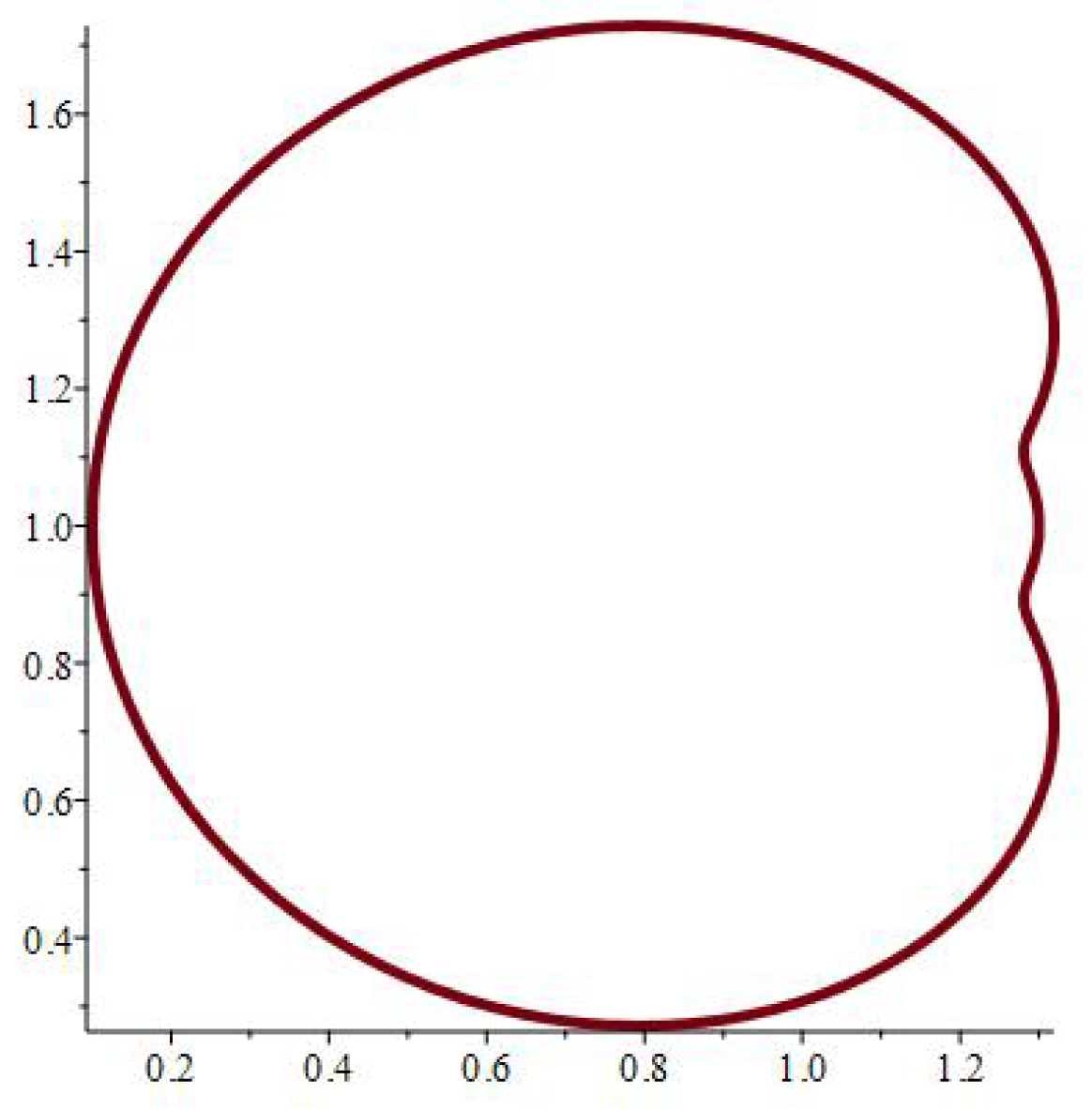
3. Conformal Mapping and Special Cases

The physical significance of mapping (1) depends on its ability to model various hole forms, as seen in Figure 2, Figure 3, Figure 4, Figure 5, Figure 6, Figure 7, Figure 8, Figure 9, Figure 10, Figure 11, Figure 12 and Figure 13, which include the following notations:

4. Method of Solution

In this section, we use the transformation mapping (1) in the boundary condition (4). We apply the complex variable method with the residue theorem to obtain a closed expression for Goursat functions [20]. Therefore, the expression Ω ( ξ ) / Ω ξ 1 will be written in the form
Ω ( ξ ) Ω ξ 1 = ρ ( ξ ) + ϱ ( ξ ) ¯ ,
where
ρ ( ξ ) = l | l | 2 j = 1 M m j ξ j ,
and ϱ ( ξ ) is a regular function for | ξ | > 1 .
Applying (12) to (4), and operating on ξ = ϑ , we have
L χ ( ϑ , τ ) ρ ( ϑ ) χ ( ϑ , τ ) ¯ ϖ ( ϑ , τ ) ¯ = g ( ϑ , τ ) ,
where
ϖ ( ϑ , τ ) = ϖ ( ϑ , τ ) + ϱ ( ϑ ) χ ( ϑ , τ ) , g ( ϑ , τ ) = G ( ϑ , τ ) l L Δ ( τ ) ϑ + l Δ ( τ ) ¯ ϑ + N ( ϑ , τ ) ( ρ ( ϑ ) + ϱ ( ϑ ) ¯ ) , N ( ϑ , τ ) = l Δ ( τ ) ¯ S x ( ϑ , τ ) i S y ( ϑ , τ ) 2 π ( 1 + κ ) ϑ ,
and
G ( ϑ , τ ) = g ( τ ) .
All derivatives of the function g ( ϑ ) must satisfy the Hölder condition. Multiplying (14) by ( 1 / 2 π i ) 1 / ( ϑ ξ ) and then integrating regarding ϑ on δ yields
L χ ( ξ , τ ) + 1 2 π i δ ρ ( ϑ ) χ ( ϑ , τ ) ¯ d ϑ ϑ ξ = Δ ( τ ) ¯ ξ + l | l | 2 j = 1 M m j ξ j N ( 0 , τ ) A ( ξ , τ ) ,
where
A ( ξ , τ ) = 1 2 π i η = 0 1 ξ n + 1 δ ϑ η G ( ϑ , τ ) d ϑ , | ξ | > 1 .
Using (13) in the integral term of (17), we have
1 2 π i z ρ ( ϑ ) χ ( ϑ , τ ) ¯ d ϑ ϑ ξ = l | l | 2 j = 1 M k = 0 j 1 1 ( j 1 ) ! j 1 k k ! m χ j k ( 0 , τ ) ¯ ξ 1 + k ,
where χ j k ( 0 , τ ) ¯ is a complex function to be established.
Substituting from (19) into (17), we obtain
L χ ( ξ , τ ) = A ( ξ , t τ ) l Δ ( τ ) ¯ ξ l | l | 2 j = 1 M k = 0 j 1 1 ( j 1 ) ! j 1 k k ! m j χ j k ( 0 , τ ) ¯ ξ 1 + k l | l | 2 j = 1 M m j ξ j N ( 0 , τ ) .
Differentiating (20) regarding ξ , and using the result in (19), we obtain
χ j k ( 0 , τ ) ¯ = 1 L A j k ( 0 , τ ) ¯ , k = 0 , 2 , , j 1 .
It is also possible to obtain ϖ ( ξ , τ ) from Equation (14) in the following way:
ϖ ( ξ , τ ) = L Δ ( τ ) ¯ ξ Ω ξ 1 Ω ( ξ ) χ ( ξ , τ ) + l ¯ | l | 2 j = 1 M k = 0 j 1 1 ( j 1 ) ! j 1 k k ! m ¯ j χ j k ( 0 , τ ) ξ 1 + k + l ¯ | l | 2 j = 1 M m ¯ j ξ j N ( 0 , τ ) ¯ + B ( ξ , τ ) B ,
where
χ ( ξ , τ ) = χ ( ξ , τ ) + N ( ξ , τ ) ¯ , B ( ξ , τ ) = 1 2 π i y G ( ϑ , τ ) ¯ ϑ ξ d ϑ ,
and
B = 1 2 π i G ( ϑ , τ ) ¯ ϑ d ϑ .

5. Applications

Application 1: Curvilinear Holes for an Infinite Plate Undergoing Uniform Tensile Stress
For L = 1 , Δ ( τ ) = Λ ( τ ) 4 , Δ ( τ ) = Λ ( τ ) 2 e 2 i θ , where Λ ( τ ) = 1 + τ 4 ( 1 τ ) , τ < 1 , θ = π 4 and S x = S y = g = 0 , a plate with infinite stretch is exposed to a uniform tensile stress with intensity Λ , resulting in the formation of an angle θ with the x-axis. A curvilinear hole S, free of stresses, weakens the plate. The functions (20)–(22) take the following forms:
χ ( ξ , τ ) = l ¯ Λ ( r ) 2 ξ Λ ( τ ) 4 j = 1 M m j ξ j ,
ϖ ( ξ , τ ) = l ¯ Λ ( τ ) 4 ξ Ω ξ 1 Ω ( ξ ) χ ( ξ ) + l Λ ( τ ) 4 + Λ ( τ ) 4 j = 1 M m ¯ j ξ j .
The figures of the two cases below demonstrate the graphical representation and large-form calculation of the three stress components ϑ x x , ϑ y y , and ϑ x y :
  • In order to calculate the stresses, this study uses the standard plate Equation (5) (see Figure 14, Figure 15, Figure 16, Figure 17 and Figure 18).
    For A : = 2 + 3 i ; m 1 : = 0.4 ; m 2 : = 0.3 , m 3 : = 0.5 , m 4 : = 0.7 , θ [ 0 , 2 π ] , τ [ 0 , 1.99 )
  • To determine the stress expressions in the thermoelasticity plate, we refer to Equation (8). So, the stresses are calculated using the replacements G = 1 2 , q = 2 , ν = 1 , α = 1 2 , r 0 = 1 2 (see Figure 19, Figure 20, Figure 21, Figure 22 and Figure 23).
For A : = 3 + 2 i ; m 1 : = 0.4 ; m 2 : = 0.3 ; m 3 : = 0.2 , θ [ 0 , 2 π ] , τ [ 0 , 0.99 )
Figure 14. The normal stress components ϑ x x versus the angle θ during variant times.
Axioms 14 00369 g014
Figure 15. The normal stress components ϑ y y versus the angle θ during variant times.
Axioms 14 00369 g015
Figure 16. The shear stress components ϑ x y versus the angle θ during variant times.
Axioms 14 00369 g016
Figure 17. Stress ratios R = ϑ m i n ϑ m a x .
Axioms 14 00369 g017
Figure 18. Stress ratios R 1 = ϑ m a x ϑ m i n .
Axioms 14 00369 g018
Figure 19. The normal stress components ϑ x x versus the angle θ during variant times under heating flow effect.
Axioms 14 00369 g019
Figure 20. The normal stress components ϑ y y versus the angle θ during variant times under heating flow effect.
Axioms 14 00369 g020
Figure 21. The shear stress components ϑ x y versus the angle θ during variant times under heating flow effect.
Axioms 14 00369 g021
Figure 22. Stress ratios R = ϑ m i n ϑ m a x .
Axioms 14 00369 g022
Figure 23. Stress ratios R 1 = ϑ m a x ϑ m i n .
Axioms 14 00369 g023
Application 2: Uni-Directional Tension of an Infinite Plate with a Rigid Curvilinear Center
For L = κ , Δ = Λ ( τ ) 4 , Δ = 1 2 Λ ( τ ) exp ( 2 i θ ) , and S x = S y = 0 , g = 2 i Λ ( τ ) ε , the two complex functions (20), (22) take the form
κ χ ( ξ , τ ) = l ¯ Λ ( τ ) 2 ξ Λ ( τ ) 4 j = 1 M m j ξ j ,
ϖ ( ξ , τ ) = κ l ¯ Λ ( τ ) 4 ξ Ω ξ 1 Ω ( ξ ) χ ( ξ ) + l Λ ( τ ) 4 + Λ ( τ ) 4 j = 1 M m ¯ j ξ j + 2 i Λ ( τ ) ε .
As a result, we obtain uni-directional tension on an infinite plate with a rigid curvilinear center. Considering the requirement that the total of the moments generated by the forces acting on the curvilinear center from all directions must equal zero, we can estimate the value of the constant ε , i.e.,
M = Re ϖ ( ξ , τ ) l Λ ( τ ) 2 e 2 i θ ξ Ω ( ξ ) d ξ = 0 .
Hence,
ε = 1 2 j 1 M j ¯ j + 1 1 2 l 1 2 + 1 4 1 2 κ κ 4 l 1 2 l 2 2 cos 0 + 1 + 1 κ l 1 l 2 sin 0 + j = 1 M j 1 2 1 4 κ + κ 4 l 2 J ¯ j + 2 1 2 + 1 4 κ κ 4 l 1 J j + 2 + 1 4 j = 1 M i = 1 M i 1 κ I j i 1 m j 1 + I ¯ j i 1 + m j 2 I i + 1 + m j 1 + I i + 1 ¯ m j 2 ,
where
J t ± = m j 1 cos t θ ± m j 2 sin t θ , J ¯ t ± = m j 2 cos t θ ± m j 1 sin t θ , I t ± = m i 1 cos t θ ± m i 2 sin t θ , I t ± ¯ = m i 2 cos t θ ± m i 1 sin t θ
Figure 24. The normal stress components ϑ x x versus the angle θ during variant times.
Axioms 14 00369 g024
Figure 25. The normal stress components ϑ y y versus the angle θ during variant times.
Axioms 14 00369 g025
Figure 26. The shear stress components ϑ x y versus the angle θ during variant times.
Axioms 14 00369 g026
Figure 27. Stress ratios R = ϑ m i n ϑ m a x .
Axioms 14 00369 g027
Figure 28. Stress ratios R 1 = ϑ m a x ϑ m i n .
Axioms 14 00369 g028
Figure 29. The normal stress components ϑ x x versus the angle θ during variant times under heating flow effect.
Axioms 14 00369 g029
Figure 30. The normal stress components ϑ y y versus the angle θ during variant times under heating flow effect.
Axioms 14 00369 g030
Figure 31. The shear stress components ϑ x y versus the angle θ during variant times under heating flow effect.
Axioms 14 00369 g031
Figure 32. Stress ratios R = ϑ m i n ϑ m a x .
Axioms 14 00369 g032
Figure 33. Stress ratios R 1 = ϑ m a x ϑ m i n .
Axioms 14 00369 g033
  • For A : = 3 + 2 i ; m 1 : = 0.4 ; m 2 : = 0.3 ; m 3 : = 0.2 , θ [ 0 , 2 π ] , τ [ 0 , 0.99 )
Taking nickel, copper, and silver, we calculate the absolute values of Goursat functions with time for these minerals. See Table 1, Table 2 and Table 3.
Figure 34, Figure 35 and Figure 36 indicate the relationship between Goursat functions and different tenses.
Application 3: When the Center of the Curvilinear is Subjected to an External Force
For Δ = Δ = g = 0 and L = κ , when the force is applied to the curvilinear kernel, we obtain the second boundary problem. It is hypothesized that stresses do not exist at limitless values, and it is readily apparent that the kernel does not undergo rotation.
In general, the kernal remains in the original position. The Goursat functions are
χ ( ξ , τ ) = 0
ϖ ( ξ , τ ) = Ω ξ 1 Ω ( ξ ) S x ( τ ) + i S y ( τ ) 2 π ( 1 + κ ) ξ 1

6. Discussion and Conclusions

In the current study, the physical model for an infinite elastic medium is presented, subjected to the uniform heat flow in the direction of a negative y-axis. In the context of thermoelastic theory under the effect of uniform stress forces, the medium weakens by multi-curvilinear holes. The complex variable method (Cauchy method) plays a main role to obtain the two Goursat functions at various times by projecting the infinite domain of the problem onto a unit circle. This technique is powerful to help deal with the infinite domain more efficiently, including the geometric interpretation and reducing the problem to a famous kind of contact problem that represents a second kind of integrodifferential equation with a discontinuous kernel (Cauchy kernel), ensuring the stability of the numerical approach. The investigations on the normal and shear stress components indicate an important area of the study. Then, the stress components and stress ratios for both the standard plate and the thermoelastic case were computed and displayed graphically in 3D for various physical applications. The theoretical knowledge and graphical results indicate that
  • In the standard case, the components of stress behave in line with the behavior of wave propagation and act as tensile forces or compression forces; see Figure 14, Figure 15, Figure 16, Figure 24, Figure 25, Figure 26, and Figure 37, Figure 38 and Figure 39.
  • In the thermoelastic case, there is a clear influence of heat conduction on the physical quantities, which appears to be oscillatory regarding the stress components; see Figure 19, Figure 20, Figure 21, Figure 29, Figure 30, Figure 31, and Figure 42, Figure 43 and Figure 44.
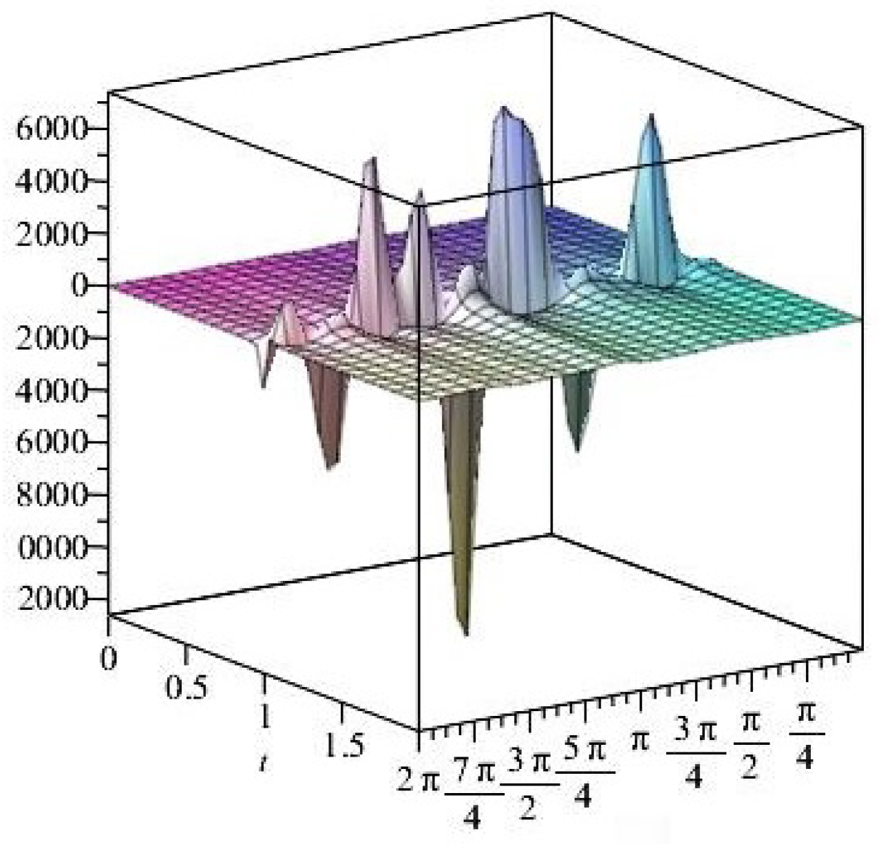
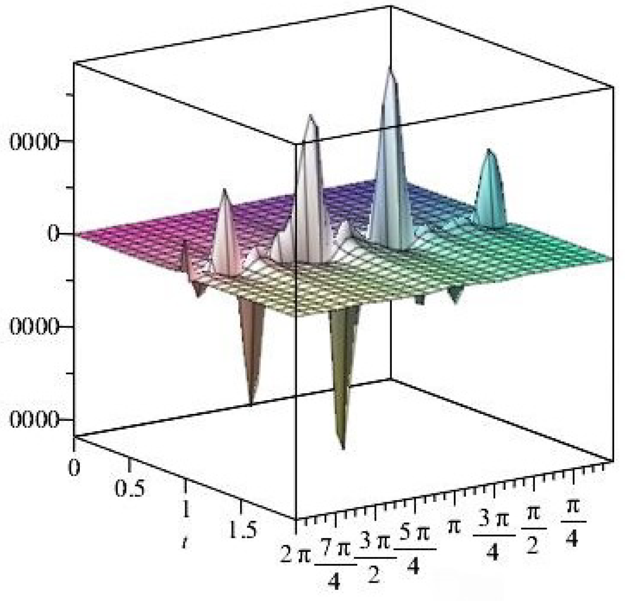
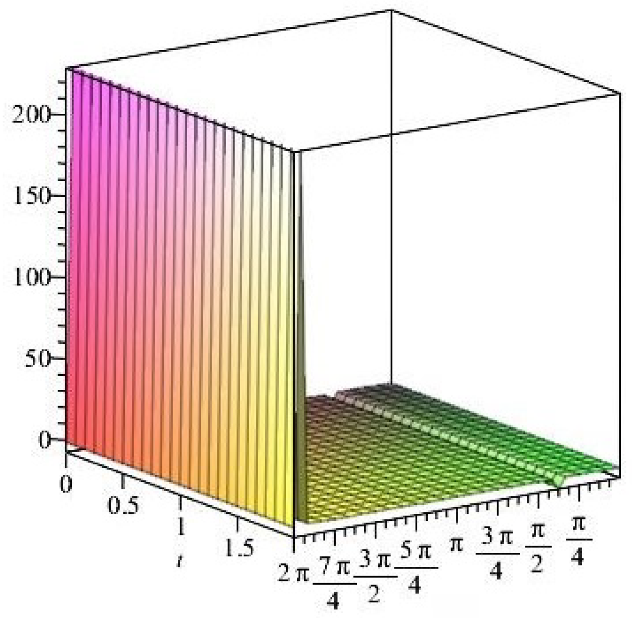
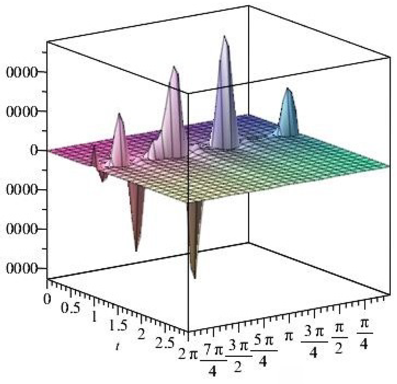
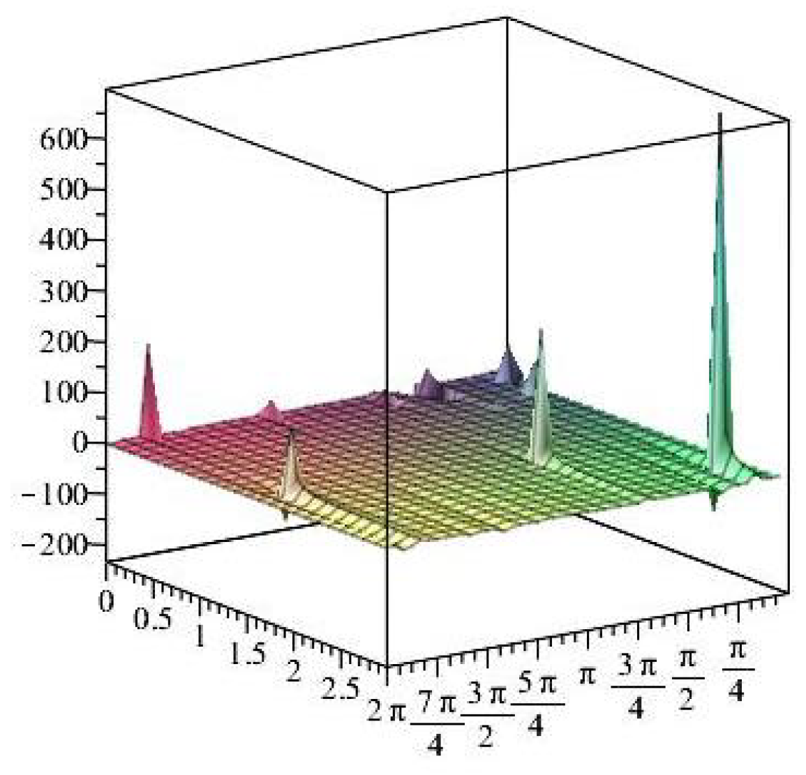
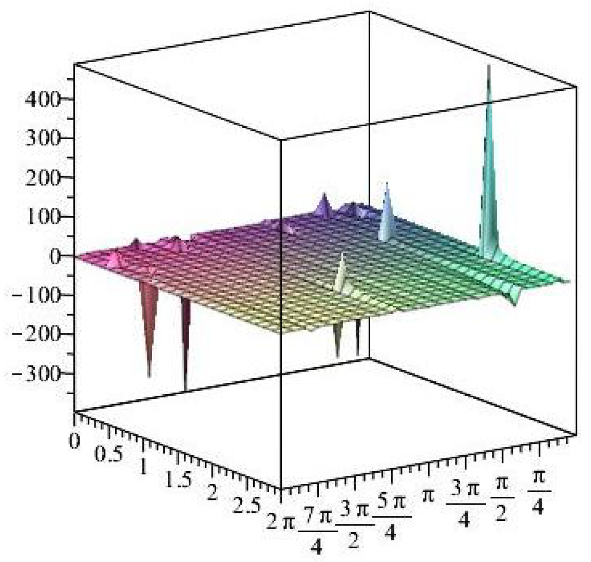
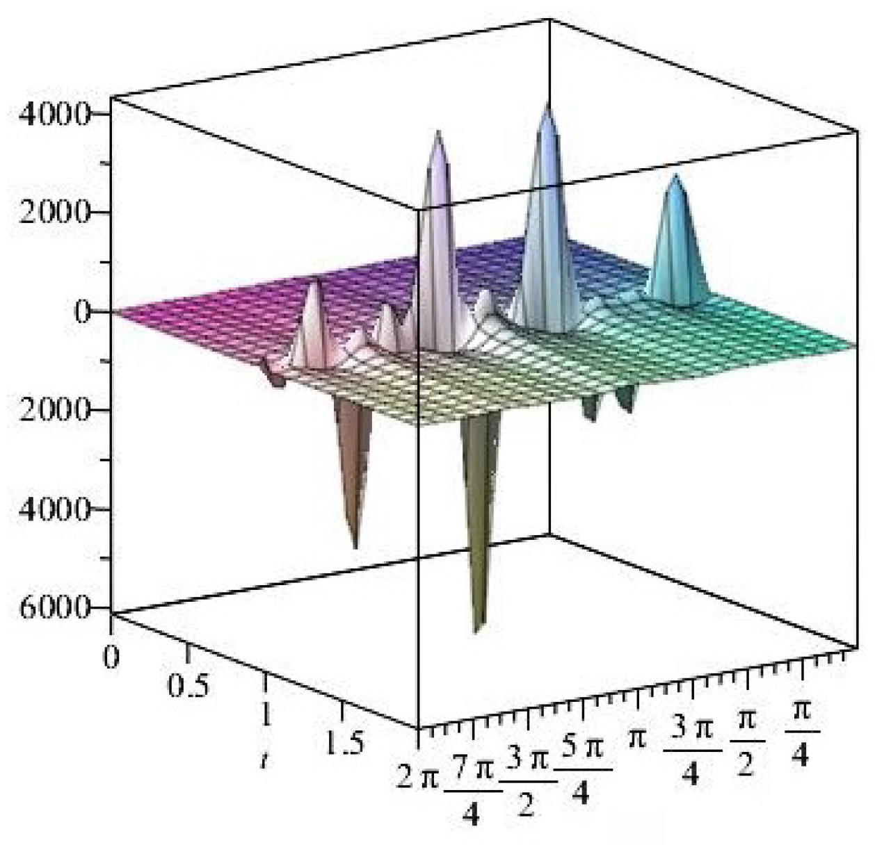
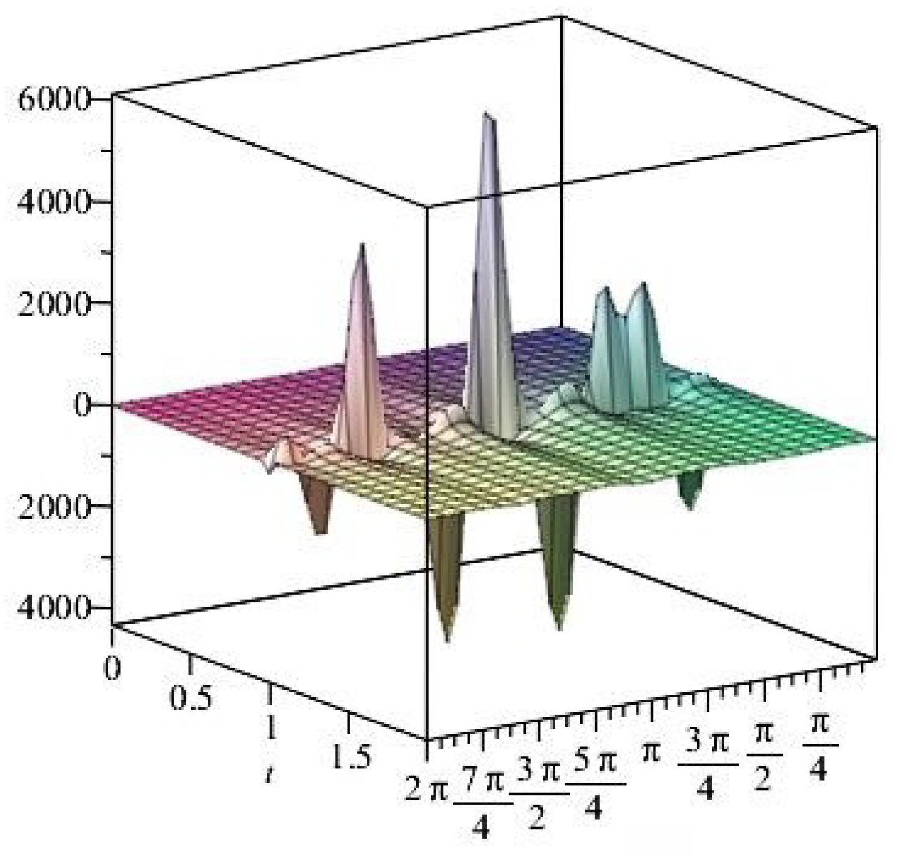
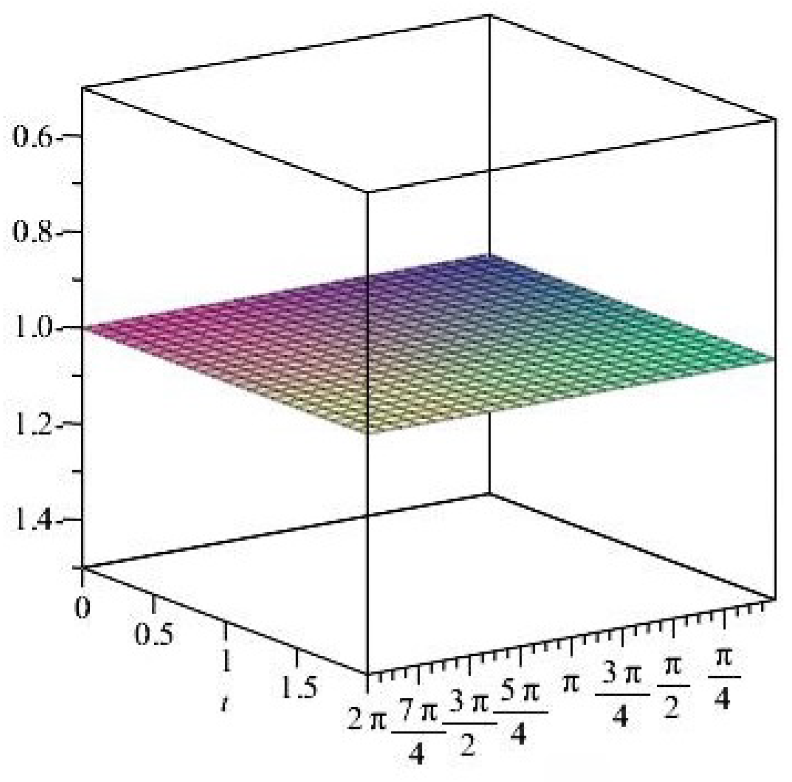
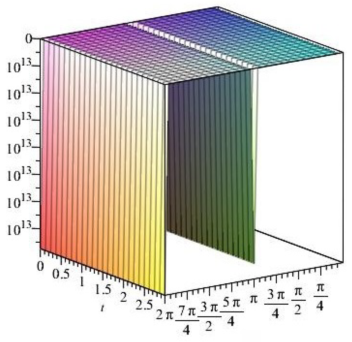
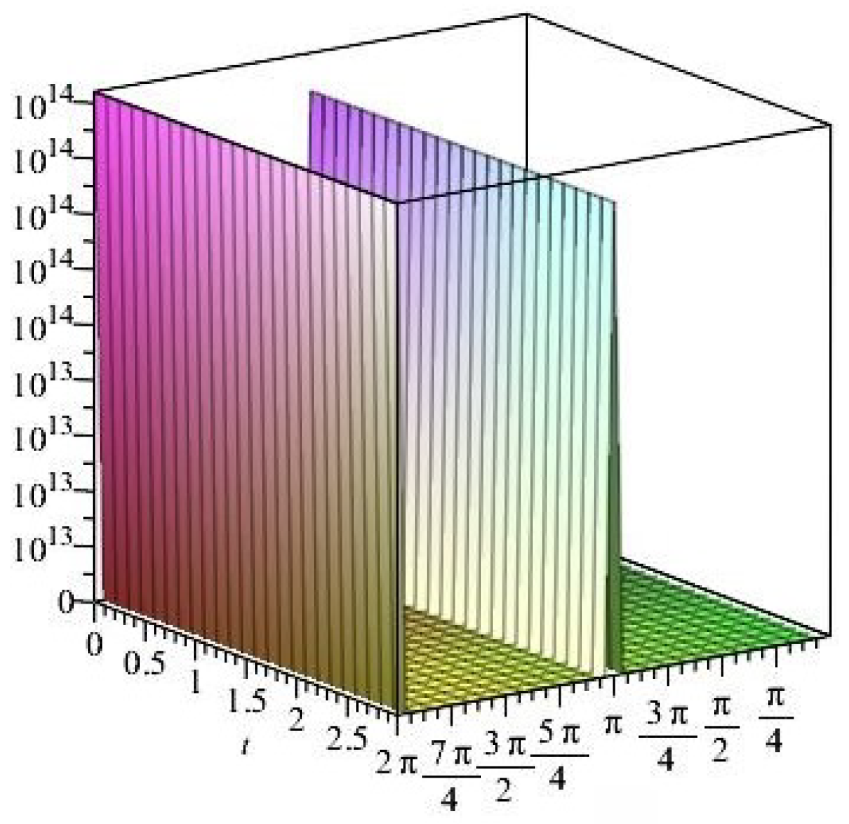
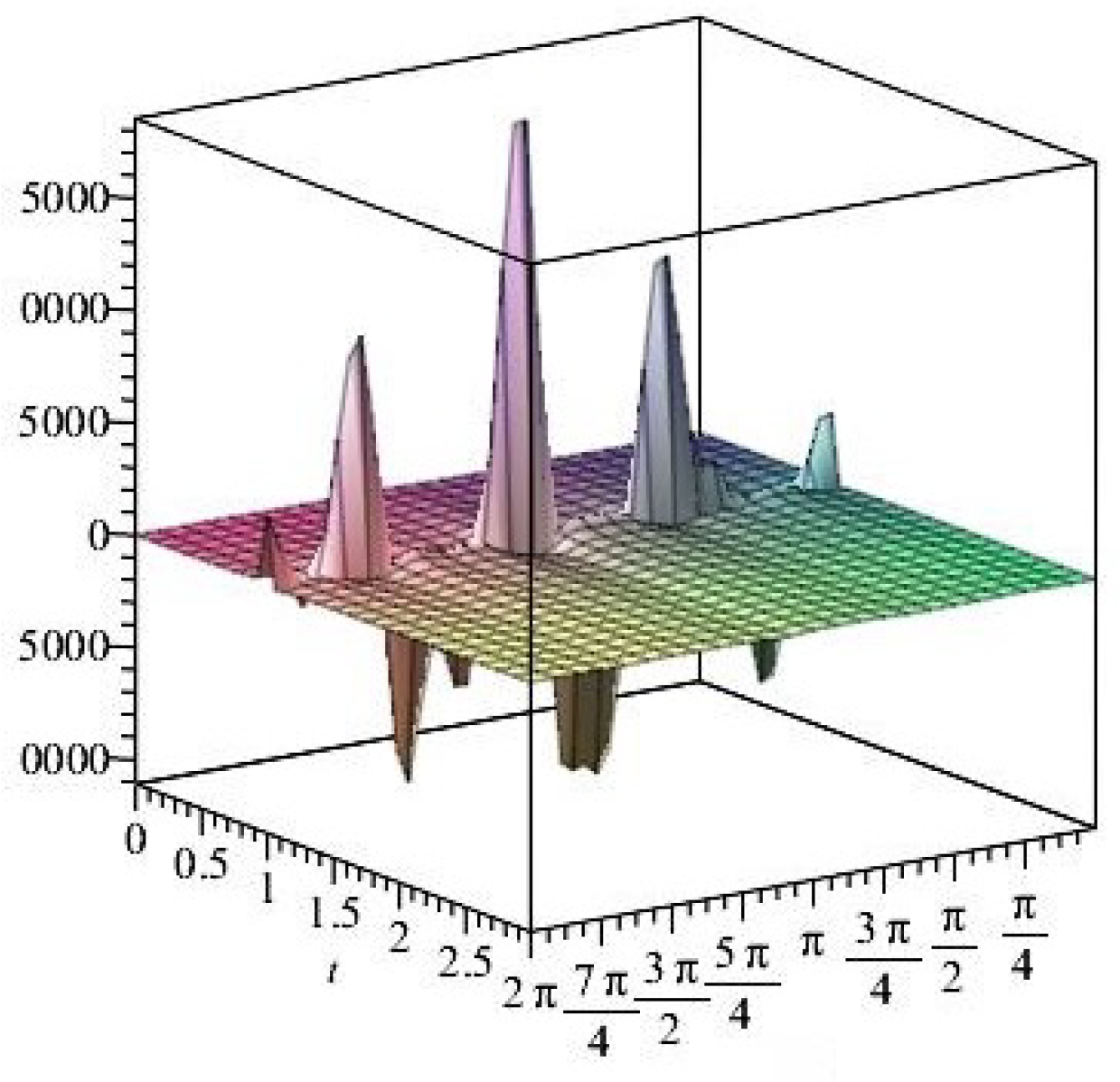
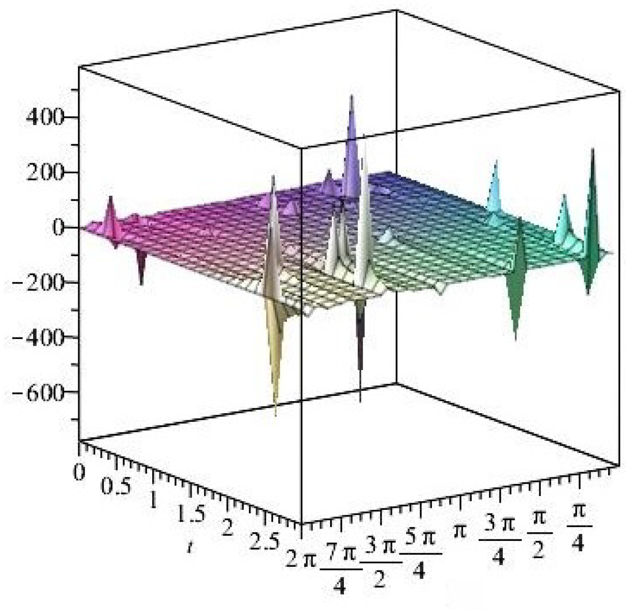
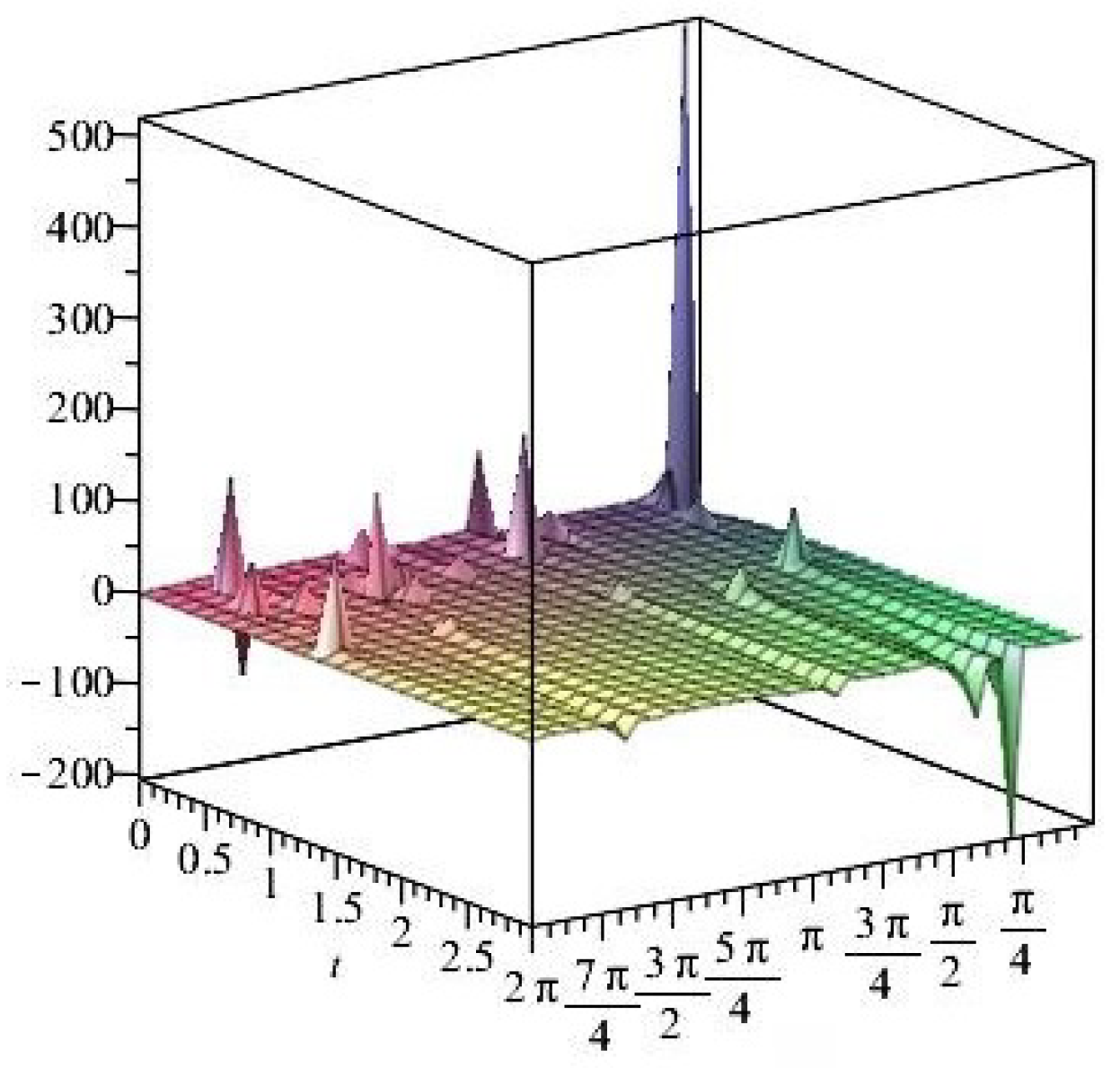
  • It is noticed from the resulting values of the stress ratios that the stress remains positive between the minimum and maximum tensile values; see Figure 17 and Figure 22, and, as a special case, when there is no stress change, then see Figure 40. Meanwhile, for a rigid curvilinear center, the stress ratios across a large surface domain are illustrated in Figure 27.
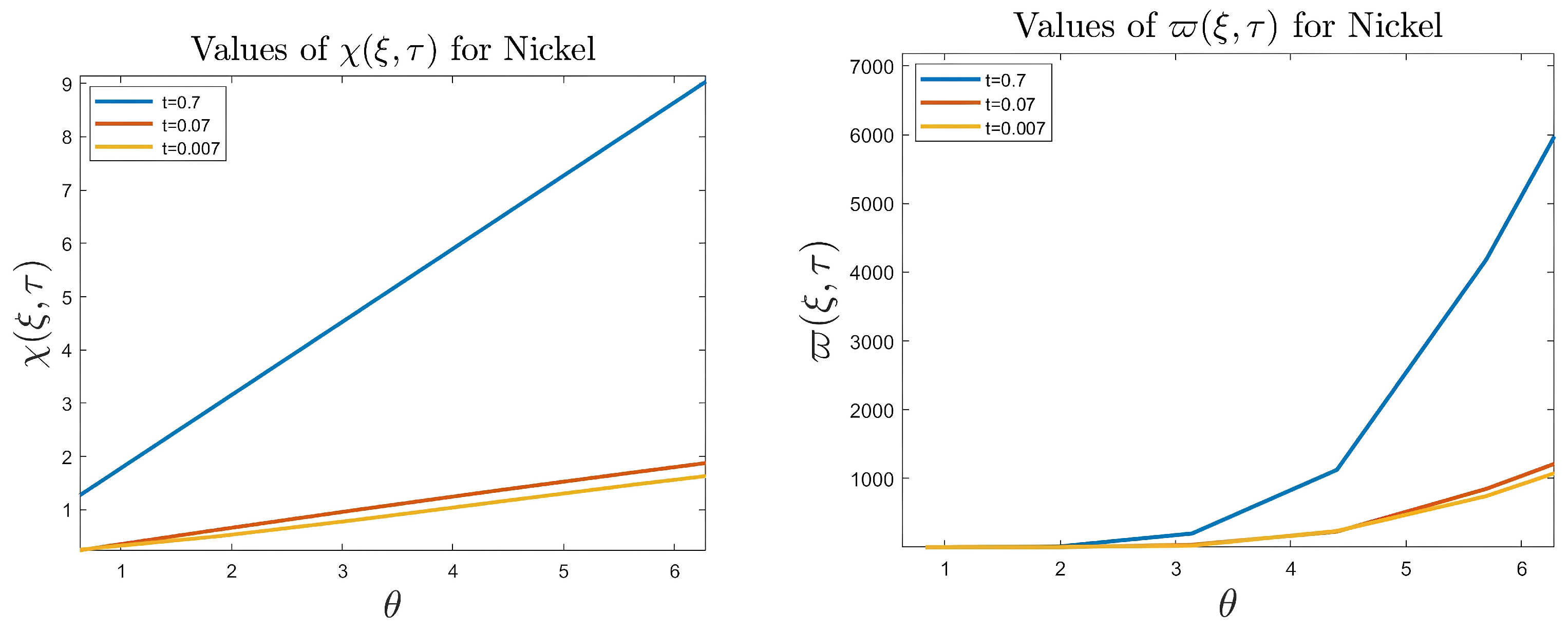
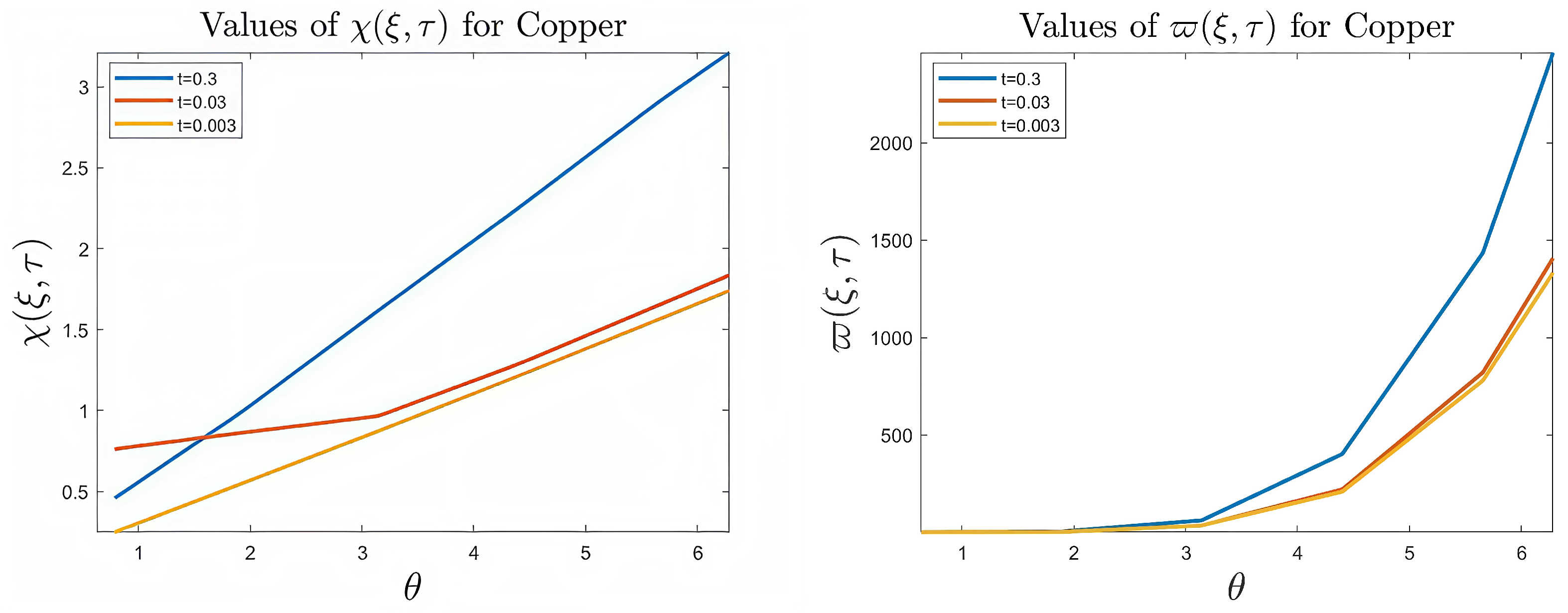
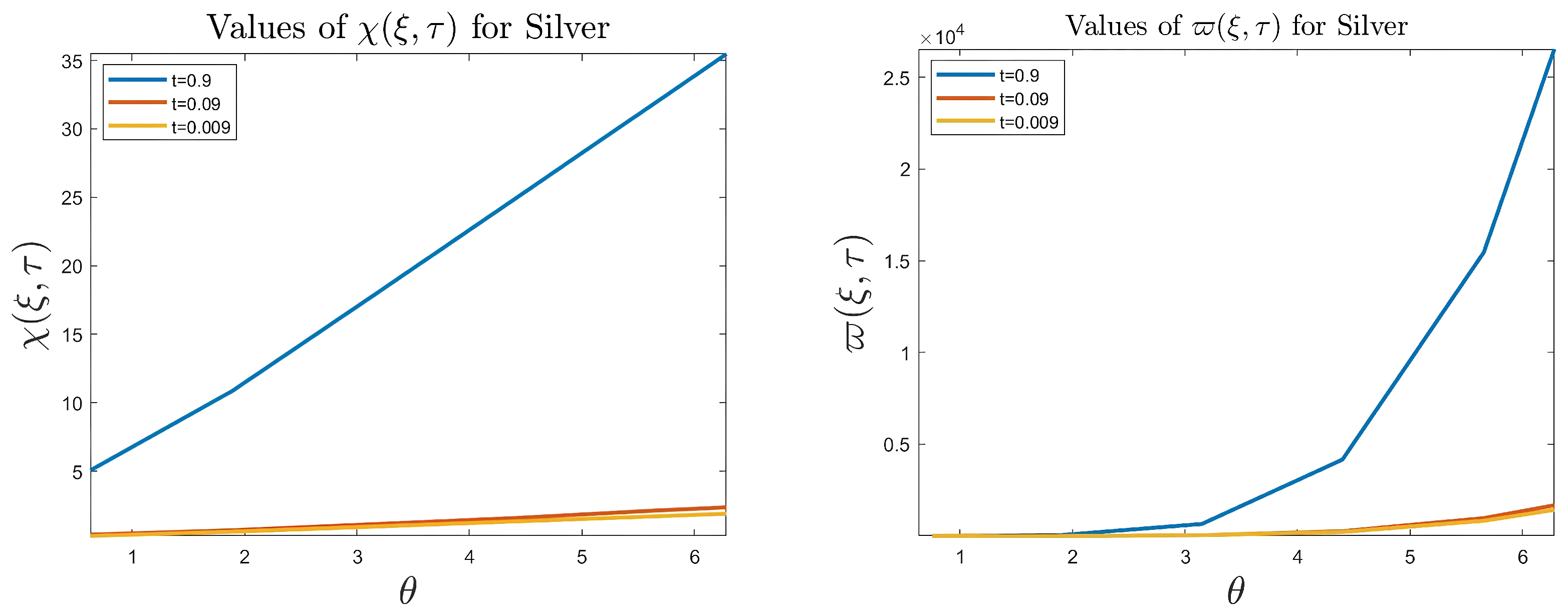
  • The numerical results indicate that, besides the boundary conditions that restricted the domain of the problem, acting stress forces, and heat conduction at various times, the two Goursat functions provide increasing values with respect to increasing time (0,1). Therefore, a general visualization of the amplitude of waves or energy levels is determined. See Table 1, Table 2 and Table 3.
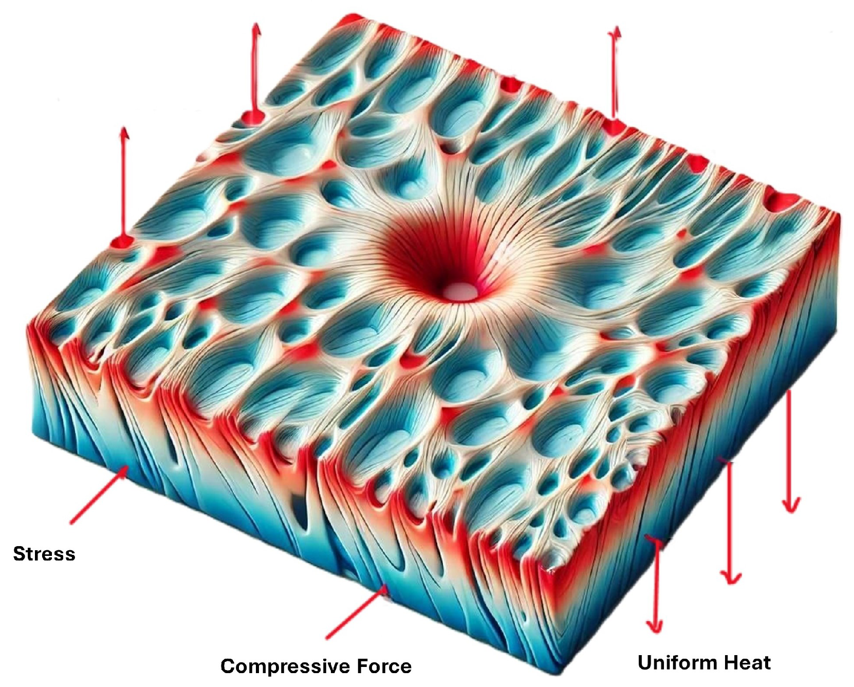
  • The current model appears in more general physical phenomena. For example, in ceramic thermoelastic plates, the coupling of many curvilinear holes in a metallic ceramic plate under the effect of uniform stress forces in the presence of heat conduction necessitates a thorough examination of both thermal and mechanical stress factors. Numerical approaches, stress intensity factors, and fracture mechanics are crucial in forecasting material performance and failure. To optimize the design and reduce the danger of failure, special attention should be paid to the hole arrangement, thermal gradient, and material qualities.
Future Work:
  • Study the physical model in the presence of a normal magnetic field.
  • Expand the study to include the effect of the external forces near the edges of the plate.

Author Contributions

Conceptualization, F.M.A.; Methodology, F.M.A. and N.G.A.; Software, N.G.A.; Formal analysis, N.G.A.; Investigation, N.G.A.; Resources, F.M.A.; Writing—original draft, N.G.A.; Writing—review & editing, N.G.A.; Supervision, F.M.A.; Project administration, F.M.A.; Funding acquisition, F.M.A. All authors have read and agreed to the published version of the manuscript.

Funding

This research received no external funding.

Data Availability Statement

Data are contained within the article.

Conflicts of Interest

The authors declare no conflict of interest.

References

  1. Nowacki, W. Thermoelasticity; Pergamon Press: Warsaw, Poland, 2013; Available online: https://shop.elsevier.com/books/thermoelasticity/nowacki/978-0-08-024767-0 (accessed on 22 October 2013).
  2. Khaldjigitov, A.; Tilovov, O.; Xasanova, Z. A new approach to problems of thermoelasticity in stresses. J. Therm. Stress. 2024, 47, 1228–1241. [Google Scholar] [CrossRef]
  3. Manickam, G.; Haboussi, M.; D’Ottavio, M.; Kulkarni, V.; Chettiar, A.; Gunasekaran, V. Nonlinear thermo-elastic stability of variable stiffness curvilinear fibres based layered composite beams by shear deformable trigonometric beam model coupled with modified constitutive equations. Int. J. Non-Linear Mech. 2023, 148, 104303. [Google Scholar] [CrossRef]
  4. Yuan, X.; Jiang, Q.; Zhou, Z.; Yang, F. Stress analysis of anti-plane finite elastic solids with hole by the method of fundamental solutions using conformal mapping technique. Arch. Appl. Mech. 2022, 92, 1823–1839. [Google Scholar] [CrossRef]
  5. Lu, A.Z.; Xu, Z.; Zhang, N. Stress analytical solution for an infinite plane containing two holes. Int. J. Mech. Sci. 2017, 128, 224–234. [Google Scholar] [CrossRef]
  6. Hsieh, M.L.; Hwu, C. Green’s functions for anisotropic elastic plates containing polygonal holes. Int. J. Mech. Sci. 2024, 276, 109396. [Google Scholar] [CrossRef]
  7. Savruk, M.P. Stress Concentration Near Curvilinear Holes and Notches with Nonsmooth Contours. Mater. Sci. 2021, 57, 331–343. [Google Scholar] [CrossRef]
  8. Hsieh, M.L.; Hwu, C. A full field solution for an anisotropic elastic plate with a hole perturbed from an ellipse. Eur. J. Mech. A/Solids 2023, 97, 104823. [Google Scholar] [CrossRef]
  9. Guo, J.; Lu, Z. Line field analysis and complex variable method for solving elastic-plastic fields around an anti-plane elliptic hole. Sci. China Phys. Mech. Astron. 2011, 54, 1495–1501. [Google Scholar] [CrossRef]
  10. Abdou, M.A. Fundamental problems for infinite plate with a curvilinear hole having finite poles. Appl. Math. Comput. 2002, 125, 79–91. [Google Scholar] [CrossRef]
  11. Abdou, M.A.; Ibrahim, E.; Basseem, M. The stress and strain components for a weakened elastic plate by two curvilinear holes in presence of heat. Curr. Sci. Int. 2022, 11, 199–216. Available online: https://www.curresweb.com/index.php/CSI1/article/view/81 (accessed on 30 May 2022).
  12. Abdou, M.A.; Monaquel, S.J. Integro Differential Equation and Fundamental Problems of an Infinite Plate with a Curvilinear Hole Having Strong Pole. Int. J. Contemp. Math. Sci. 2011, 6, 199–208. Available online: https://www.researchgate.net/profile/M-Abdou-3/publication/267677313_Integro_differential_equation_and_fundamental_problems_of_an_infinite_plate_with_a_curvilinear_hole_having_strong_pole/links/5523e5c80cf2c815e073650b/Integro-differential-equation-and-fundamental-problems-of-an-infinite-plate-with-a-curvilinear-hole-having-strong-pole.pdf (accessed on 1 January 2011).
  13. Mattei, O.; Lim, M. Explicit analytic solution for the plane elastostatic problem with a rigid inclusion of arbitrary shape subject to arbitrary far-field loadings. J. Elast. 2021, 144, 81–105. [Google Scholar] [CrossRef]
  14. Alhazmi, S.; Abdou, M.A.; Basseem, M. The stresses components in position and time of weakened plate with two holes conformally mapped into a unit circle by a conformal mapping with complex constant coefficients. AIMS Math. 2023, 8, 11095–11112. Available online: https://www.aimspress.com/aimspress-data/math/2023/5/PDF/math-08-05-562.pdf (accessed on 9 March 2023). [CrossRef]
  15. Trefethen, L.N. Numerical conformal mapping with rational functions. Comput. Methods Funct. Theory 2020, 20, 369–387. [Google Scholar] [CrossRef]
  16. Alharbi, F.M.; Alhendi, N.G. New Approach of Normal and Shear Stress Components for Multiple Curvilinear Holes Which Weakened a Flexible Plate. Symmetry 2024, 16, 360. [Google Scholar] [CrossRef]
  17. Jan, A.R. The solution of a complex integro differential equation in the right half-plane via an infinite plate weakened by a curvilinear hole. Appl. Math. 2024, 18, 493–503. [Google Scholar] [CrossRef]
  18. Parkus, H. Thermoelasticity; Springer: Berlin, Germany, 1976. [Google Scholar] [CrossRef]
  19. Abdou, M.A.; Basseem, M. Thermopotential function in position and time for a plate weakened by curvilinear hole. Arch. Appl. Mech. 2022, 92, 867–883. [Google Scholar] [CrossRef]
  20. Abdou, M.A.; Aseeri, S.A. Closed forms of Goursat functions in presence of heat for curvilinear holes. J. Therm. Stress. 2009, 32, 1126–1148. [Google Scholar] [CrossRef]
Figure 1. Physical description of the problem.
Axioms 14 00369 g001
Figure 2. A = 1 + i ; m 1 = 0.5 ; m 2 = 0.1 ; m 3 = 0.3 ; m 4 = 0 .
Axioms 14 00369 g002
Figure 3. A = 1 i ; m 1 = 0.4 ; m 2 = 0.2 .
Axioms 14 00369 g003
Figure 4. A = 1 5 i ; m 1 = 0.4 ; m 2 = 0.2 ; m 3 = 0.1 .
Axioms 14 00369 g004
Figure 5. A = 2 + i ; m 1 = 0.2 ; m 2 = 0.1 .
Axioms 14 00369 g005
Figure 6. A = 5 ; m 1 = 0.4 ; m 2 = 0.2 ; m 3 = 0.1 .
Axioms 14 00369 g006
Figure 7. A = 1 + i ; m 1 = 0.6 ; m 2 = 0.3 .
Axioms 14 00369 g007
Figure 8. A = 2 i ; m 1 = 0.8 ; m 2 = 0.4 .
Axioms 14 00369 g008
Figure 9. A = 8 + 3 i ; m 1 = 0.9 ; m 2 = 0.45 .
Axioms 14 00369 g009
Figure 10. A = 1 + i ; m 1 = 0.4 ; m 2 = 0.3 ; m 3 = 0.2 ; m 4 = 0.1 .
Axioms 14 00369 g010
Figure 11. A = 1 + i ; m 1 = 0.8 ; m 2 = 0.6 ; m 3 = 0.4 ; m 4 = 0.2 .
Axioms 14 00369 g011
Figure 12. A = 1 i ; m 1 = 0.8 ; m 2 = 0.4 .
Axioms 14 00369 g012
Figure 13. A = 1 i ; m 1 = 0.4 ; m 2 = 0.2 .
Axioms 14 00369 g013
Figure 34. Values of χ ( ξ , τ ) and f ϖ ( ξ , τ ) for nickel, where κ = 91 Wm 1 k 1 .
Axioms 14 00369 g034
Figure 35. Values of χ ( ξ , τ ) and f ϖ ( ξ , τ ) for copper, where κ = 402 Wm 1 k 1 .
Axioms 14 00369 g035
Figure 36. Values of χ ( ξ , τ ) and f ϖ ( ξ , τ ) for silver, where κ = 436 Wm 1 k 1 .
Axioms 14 00369 g036
Figure 37. The normal stress components ϑ x x versus the angle θ during variant times.
Axioms 14 00369 g037
Figure 38. The normal stress components ϑ y y versus the angle θ during variant times.
Axioms 14 00369 g038
Figure 39. The shear stress components ϑ x y versus the angle θ during variant times.
Axioms 14 00369 g039
Figure 40. Stress ratios R = ϑ m i n ϑ m a x .
Axioms 14 00369 g040
Figure 41. Stress ratios R 1 = ϑ m a x ϑ m i n .
Axioms 14 00369 g041
Figure 42. The normal stress components ϑ x x versus the angle θ during variant times under heating flow effect.
Axioms 14 00369 g042
Figure 43. The normal stress components ϑ y y versus the angle θ during variant times under heating flow effect.
Axioms 14 00369 g043
Figure 44. The shear stress components ϑ x y versus the angle θ during variant times under heating flow effect.
Axioms 14 00369 g044
Figure 45. Stress ratios R = ϑ n i m ϑ m a x .
Axioms 14 00369 g045
Figure 46. Stress ratios R 1 = ϑ y y ϑ x x .
Axioms 14 00369 g046
Table 1. Values of | χ ( ξ , τ ) | and | ϖ ( ξ , τ ) | for nickel, where ( κ = 91 Wm 1 k 1 ).
at τ = 0.7at τ = 0.07at τ = 0.007
ξ χ ξ , τ ϖ ξ , τ χ ξ , τ ϖ ξ , τ χ ξ , τ ϖ ξ , τ
22 35 0.025220037184.08790695.12 × 10−337.376482034.51 × 10−332.94411269
66 35 0.05398422351.543082340.01096074410.465104019.66 × 10−39.224077468
22 7 0.088736947153.4208470.0180167131.14996320.015880239227.45597877
198 35 0.1590317813477.816320.32289185706.1220990.028460104622.385114
44 7 0.1766430945972.5820.0358649161212.649450.03161179951068.8449
Table 2. Values of | χ ( ξ , τ ) | and | ϖ ( ξ , τ ) | for copper, where ( κ = 402 Wm 1 k 1 ).
at τ = 0.3at τ = 0.03at τ = 0.003
ξ χ ξ , τ ϖ ξ , τ χ ξ , τ ϖ ξ , τ χ ξ , τ ϖ ξ , τ
22 35 1.87 × 10−3267.3951281.06 × 10−3152.8880951.01 × 10−3144.848484
66 35 4.004 × 10−385.876752.28 × 10−349.10161522.17 × 10−346.519609
22 7 6.58 × 10−375.6169983.76 × 10−343.235413223.56 × 10−340.9618816
198 35 0.01179823131155.1587746.745 × 10−3660.483326.39 × 10−3625.751852
44 7 0.0131047771977.2655287.49 × 10−31130.538027.098 × 10−31071.08874
Table 3. Values of | χ ( ξ , τ ) | and | ϖ ( ξ , τ ) | for silver, where ( κ = 436 Wm 1 k 1 ).
at τ = 0.9at τ = 0.09at τ = 0.009
ξ χ ξ , τ ϖ ξ , τ χ ξ , τ ϖ ξ , τ χ ξ , τ ϖ ξ , τ
22 35 5.0625516912967.253221.113 × 10−3187.06223319.45 × 10−4159.0078336
66 35 0.03777875955.775692.38 × 10−360.25422232.024 × 10−351.217678
22 7 0.062099102810.2534443.914 × 10−351.08017663.327 × 10−343.41949785
198 35 0.11129220811,829.252337.016 × 10−3745.742335.963 × 10−3633.90066
44 7 0.123616820240.3467.7931 × 10−31275.99646.624 × 10−31084.6305
Disclaimer/Publisher’s Note: The statements, opinions and data contained in all publications are solely those of the individual author(s) and contributor(s) and not of MDPI and/or the editor(s). MDPI and/or the editor(s) disclaim responsibility for any injury to people or property resulting from any ideas, methods, instructions or products referred to in the content.

