Flexible and Efficient Iterative Solutions for General Variational Inequalities in Real Hilbert Spaces

Abstract

This paper introduces a novel Picard-type iterative algorithm for solving general variational inequalities in real Hilbert spaces. The proposed algorithm enhances both the theoretical framework and practical applicability of iterative algorithms by relaxing restrictive conditions on parametric sequences, thereby expanding their scope of use. We establish convergence results, including a convergence equivalence with a previous algorithm, highlighting the theoretical relationship while demonstrating the increased flexibility and efficiency of the new approach. The paper also addresses gaps in the existing literature by offering new theoretical insights into the transformations associated with variational inequalities and the continuity of their solutions, thus paving the way for future research. The theoretical advancements are complemented by practical applications, such as the adaptation of the algorithm to convex optimization problems and its use in real-world contexts like machine learning. Numerical experiments confirm the proposed algorithm’s versatility and efficiency, showing superior performance and faster convergence compared to an existing method.

1. Introduction

In this paper, we adopt the standard notation for a real Hilbert space $\mathcal{H}$. The inner product on $\mathcal{H}$ is denoted by $〈·,·〉$, and the associated norm is represented by $∥·∥$. Let H denote a nonempty, closed, and convex subset of $\mathcal{H}$, and let T, $g:\mathcal{H}\to \mathcal{H}$ be two nonlinear operators. The operator $T:H\subset \mathcal{H}\to \mathcal{H}$ is called

(i)

λ-Lipschitzian if there exists a constant $\lambda >0$, such that

$$(\forall x,y\in H)∥Tx-Ty∥\le \lambda ∥x-y∥;$$

(1)

(ii)

Nonexpansive if

$$(\forall x,y\in H)∥Tx-Ty∥\le ∥x-y∥;$$

(2)

(iii)

α-inverse strongly monotonic if there exists a constant $\alpha >0$, such that

$$(\forall x,y\in H)〈Tx-Ty,x-y〉\ge \alpha {∥Tx-Ty∥}^2;$$

(3)

(iv)

r-strongly monotonic if there exists a constant $r>0$, such that

$$(\forall x,y\in H)〈Tx-Ty,x-y〉\ge r{∥x-y∥}^2;$$

(iv)

Relaxed $(\gamma ,r)$ cocoercive if there exist constants $\gamma >0$ and $r>0$, such that

$$(\forall x,y\in H)〈Tx-Ty,x-y〉\ge -\gamma {∥Tx-Ty∥}^2+r{∥x-y∥}^2.$$

(4)

It is evident that the classes of $\alpha$-inverse strongly monotonic and r-strongly monotonic mappings are subsets of the class of relaxed $\left(\gamma ,r\right)$ cocoercive mappings; however, the reverse implication does not hold.

Example 1.

Let $\mathcal{H}=\mathbb{R}$ and $H=\left[1/\sqrt{3},\infty \right)$. Clearly, $\mathcal{H}=\mathbb{R}$ is a Hilbert space with norm $∥x∥=\left|x\right|$ induced by the inner product $〈x,y〉=x·y$. Define the operator $T:\left[1/\sqrt{3},\infty \right)\to \mathbb{R}$ by $Tx=-x^3+10$.

We demonstrate that T is relaxed $\left(\gamma ,r\right)$ cocoercive with $\gamma =2$ and $r=1$. Specifically, we aim to verify that for all $x,y\in \left[1/\sqrt{3},\infty \right)$,

$$〈Tx-Ty,x-y〉+2{∥Tx-Ty∥}^2-{∥x-y∥}^2\ge 0.$$

First, note that $〈Tx-Ty,x-y〉=〈-x^3+y^3,x-y〉=-{(x-y)}^2\left(x^2+xy+y^2\right)$, and

$$\gamma {∥Tx-Ty∥}^2-r{∥x-y∥}^2=2{\left(x-y\right)}^2{\left(x^2+xy+y^2\right)}^2-{\left(x-y\right)}^2.$$

Combining the terms, for all $x,y\in [1/\sqrt{3},\infty )$, we see that

$$\begin{array}{cc}\hfill 〈Tx-Ty,x-y〉& +2{∥Tx-Ty∥}^2-{∥x-y∥}^2\hfill \\ \hfill & =-{\left(x-y\right)}^2\left(x^2+xy+y^2\right)+2{\left(x-y\right)}^2{\left(x^2+xy+y^2\right)}^2-{\left(x-y\right)}^2\hfill \\ \hfill & ={(x-y)}^2\left[2{\left(x^2+xy+y^2\right)}^2-\left(x^2+xy+y^2\right)-1\right]\ge 0.\hfill \end{array}$$

Indeed, putting $X=x^2+xy+y^2$, we conclude that

$$2{\left(x^2+xy+y^2\right)}^2-\left(x^2+xy+y^2\right)-1=2X^2-X-1=(2X+1)(X-1)\ge 0,$$

because $X\ge 1$ for all $x,y\in [1/\sqrt{3},\infty )$. Thus, T is relaxed $(2,1)$ cocoercive.

Since $〈Tx-Ty,x-y〉=-{\left(x-y\right)}^2\left(x^2+xy+y^2\right)\le 0$ for all $x,y\in \left[1/\sqrt{3},\infty \right)$, we conclude that there is no positive constant α, such that (3) holds. Thus, the operator T is not α-inverse strongly monotonic. Also, it is not an r-strongly monotonic.

The theory of variational inequalities, initially introduced by Stampacchia [1] in the context of obstacle problems in potential theory, provides a powerful framework for addressing a broad spectrum of problems in both pure and applied sciences. Stampacchia’s pioneering work revealed that the minimization of differentiable convex functions associated with such problems can be characterized by inequalities, thus establishing the foundation for variational inequality theory. The classical variational inequality problem (VIP) is commonly stated as follows:

Find $u\in H$ such that

$$(\forall v\in H)〈Tu,v-u〉\ge 0,$$

(5)

where $T:H\subset \mathcal{H}\to \mathcal{H}$ is a given operator. The VI (5) and its solution set are denoted by VI$(H,T)$ and $\mathsf{\Omega }(H,T)=\{u\in H:〈Tu,v-u〉\ge 0,\forall v\in H\}$, respectively.

Lions and Stampacchia [2] further expanded this theory, demonstrating its deep connections to other classical mathematical results, including the Riesz–Fréchet representation theorem and the Lax–Milgram lemma. Over time, the scope of variational inequality theory has been extended and generalized, becoming an indispensable tool for the analysis of optimization problems, equilibrium systems, and dynamic processes in a variety of fields. The historical development of variational principles, with contributions from figures such as Euler, Lagrange, Newton, and the Bernoulli brothers, highlights their profound impact on the mathematical sciences. These principles serve as the foundation for solving maximum and minimum problems across diverse disciplines such as mechanics, game theory, economics, general relativity, transportation, and machine learning. Both classical and contemporary studies emphasize the importance of variational methods in solving differential equations, modeling physical phenomena, and formulating unified theories in elementary particle physics. The remarkable versatility of variational inequalities stems from their ability to provide a generalized framework for tackling a wide range of problems, thereby advancing both theoretical insights and computational techniques.

Consequently, the theory of variational inequalities has garnered significant attention over the past three decades, with substantial efforts directed towards its development in various directions [3,4,5,6,7,8,9,10,11,12,13,14,15,16,17]. Building on this rich foundation, Noor [18] introduced a significant extension of variational inequalities known as the general nonlinear variational inequality (GNVI), formulated as follows:

Find $u\in H$ such that

$$(\forall v\in \mathcal{H}\mathit{and}g\left(v\right),g\left(u\right)\in H)〈Tu,g\left(v\right)-g\left(u\right)〉\ge 0.$$

(6)

The GNVI (6) and its solution set are denoted by GNVI$\left(H,T,g\right)$ and $\mathsf{\Omega }(H,T,g)=\left\{u\in H:〈Tu,g\left(v\right)-g\left(u\right)〉\ge 0,\forall v\in \mathcal{H},g\left(v\right),g\left(u\right)\in H\right\}$, respectively. It has been shown in Ref. [18] that problem (6) reduces to VI$\left(H,T\right)$, where $g\equiv I$ (the identity operator). Furthermore, the GNVI problem can be reformulated as a general nonlinear complementarity problem:

Find $u\in \mathcal{H}$ such that

$$〈Tu,g\left(u\right)〉=0,g\left(u\right)\in H,Tu\in H^{†},$$

(7)

where $H^{†}=\{u\in \mathcal{H}:〈u,v〉\ge 0for each v\in H\}$ is the dual cone of a convex cone H in $\mathcal{H}$. For $g\left(u\right)=m\left(u\right)+H$, where m is point-to-point mapping, problem (7) corresponds to the implicit (quasi-)complementarity problem.

A wide range of problems arising in various branches of pure and applied sciences have been studied within the unified framework of the GNVI problem (6) (see Refs. [1,19,20,21]). As an illustration of its application in differential equation theory, Noor [22] successfully formulated and studied the following third-order implicit obstacle boundary value problem:

Find $x\mapsto u\left(x\right)$ such that on $\mathsf{\Lambda }=[0,1]$

$$\left.\begin{array}{c}-u^{‴}\ge f\left(x\right),u\ge \psi \left(x\right),\hfill \\ \left(-u^{‴}-f\left(x\right)\right)\left(u-\psi \left(x\right)\right)=0,\hfill \\ u\left(0\right)=0,u^{\prime }\left(0\right),u^{\prime }\left(1\right)=0,\hfill \end{array}\right\}$$

where $\psi \left(x\right)$ is an obstacle function and $f\left(x\right)$ is a continuous function.

The projection operator technique enables the establishment of an equivalence between the variational inequality VI$\left(H,T\right)$ and fixed-point problems, as follows:

Lemma 1.

Let $P_H:\mathcal{H}\to H$ be a projection (which is also nonexpansive). For given $z\in \mathcal{H}$, the condition

$$(\forall v\in H)〈u-z,v-u〉\ge 0,$$

is equivalent to $u=P_H\left[z\right]$. This implies that

$$u\in \mathit{VI}\left(H,T\right)\iff u=P_H\left[u-\sigma Tu\right],$$

where $\sigma >0$ is a constant.

Applying this lemma to the GNVI problem (6), Noor [18] derived the following equivalence result, which establishes a connection between the GNVI and fixed-point problems:

Lemma 2.

Let $P_H:\mathcal{H}\to H$ be a projection (which is also nonexpansive). A function $u\in \mathcal{H}$ satisfies the GNVI problem (6) if and only if it satisfies the relation

$$g\left(u\right)=P_H\left[g\left(u\right)-\sigma Tu\right],$$

(8)

where $\sigma >0$ is a constant.

This equivalence has played a crucial role in the development of efficient methods for solving GNVI problems and related optimization problems. Noor [22] showed that the relation (8) can be rewritten as

$$u=u-g\left(u\right)+P_H\left[g\left(u\right)-\sigma Tu\right],$$

which implies that

$$\begin{array}{cc}\hfill u& =Su=u-g\left(u\right)+P_H\left[g\left(u\right)-\sigma Tu\right]\hfill \\ \hfill & =S\{u-g\left(u\right)+P_H\left[g\left(u\right)-\sigma Tu\right]\},\hfill \end{array}$$

(9)

where $S:H\to H$ is a nonexpansive operator and $F\left(S\right)$ denotes the set of fixed points of S.

Numerous iterative methods have been proposed for solving variational inequalities and variational inclusions [22,23,24,25,26,27,28,29,30,31]. Among these, Noor [22] introduced an iterative algorithm based on the fixed-point formulation (9) to find a common solution to both the general nonlinear variational inequality GNVI and the fixed-point problem. The algorithm is described as follows:

$$\left.\begin{array}{c}{x}_0^{\left(1\right)}\in H,\hfill \\ z_n^{\left(1\right)}=\left(1-c_n\right)x_n^{\left(1\right)}+c_{n}S\left\{x_n^{\left(1\right)}-g\left(x_n^{\left(1\right)}\right)+P_H\left[g\left(x_n^{\left(1\right)}\right)-\sigma T{x}_n^{\left(1\right)}\right]\right\},\hfill \\ y_n^{\left(1\right)}=\left(1-b_n\right)x_n^{\left(1\right)}+b_{n}S\left\{z_n^{\left(1\right)}-g\left(z_n^{\left(1\right)}\right)+P_H\left[g\left(z_n^{\left(1\right)}\right)-\sigma T{z}_n^{\left(1\right)}\right]\right\},\hfill \\ x_{n+1}^{\left(1\right)}=\left(1-a_n\right)x_n^{\left(1\right)}+a_{n}S\left\{y_n^{\left(1\right)}-g\left(y_n^{\left(1\right)}\right)+P_H\left[g\left(y_n^{\left(1\right)}\right)-\sigma T{y}_n^{\left(1\right)}\right]\right\}.\hfill \end{array}\right\}$$

(10)

where ${\left\{a_n\right\}}_{n=0}^{\infty }$, $\{b_n{\}}_{n=0}^{\infty }$, and ${\left\{c_n\right\}}_{n=0}^{\infty }$$\subset [0,1]$.

The convergence of this algorithm was established in [22] under the following conditions:

Theorem 1.

Let $T:H\to \mathcal{H}$ be a relaxed $\left(\gamma ,r\right)$ cocoercive and λ-Lipschitzian mapping, $g:H\to \mathcal{H}$ be a relaxed $\left({\gamma }_1,r_1\right)$ cocoercive and ${\lambda }_1$-Lipschitzian mapping, and $S:H\to H$ be a nonexpansive mapping such that $F\left(S\right)\cap \mathsf{\Omega }\left(H,T,g\right)\ne \varnothing$. Define ${\left\{x_n^{\left(1\right)}\right\}}_{n=0}^{\infty }$ as the sequence generated by the algorithm in (10), with real sequences ${\left\{a_n\right\}}_{n=0}^{\infty }$, $\{b_n{\}}_{n=0}^{\infty }$, and ${\left\{c_n\right\}}_{n=0}^{\infty }\subset [0,1]$, where $\sum _{n=0}^{\infty }{a}_n=\infty$. Suppose the following conditions are satisfied

$$\left|\sigma -{\displaystyle \frac{r-\gamma {\lambda }^2}{{\lambda }^2}}\right|<{\displaystyle \frac{\sqrt{{\left(r-\gamma \lambda \right)}^2-{\lambda }^{2}L\left(2-L\right)}}{{\lambda }^2}},r>\gamma {\lambda }^2+\lambda \sqrt{L\left(2-L\right)},L<1,$$

where

$$L=2\sqrt{1+2{\gamma }_1{\lambda }_1^2-2r_1+{\lambda }_1^2}.$$

Then, ${\left\{x_n^{\left(1\right)}\right\}}_{n=0}^{\infty }$ converges strongly to a solution $s_{\ast }\in F\left(S\right)\cap \mathsf{\Omega }\left(H,T,g\right)$.

Noor’s algorithm in (10) and its variants have been widely studied and applied to variational inclusions, variational inequalities, and related optimization problems. These algorithms are recognized for their efficiency and flexibility, contributing significantly to the field of variational inequalities. However, there remains considerable potential for developing more robust and broadly applicable iterative algorithms for solving GNVI problems. Motivated by the limitations of existing methods, we propose a novel Picard-type iterative algorithm designed to address general variational inequalities and nonexpansive mappings:

$$\left.\begin{array}{c}{x}_0\in H,\hfill \\ z_n=\left(1-c_n\right)x_n+c_{n}S\left\{x_n-g\left(x_n\right)+P_H\left[g\left(x_n\right)-\sigma T{x}_n\right]\right\},\hfill \\ y_n=\left(1-b_n\right)S\left\{x_n-g\left(x_n\right)+P_H\left[g\left(x_n\right)-\sigma T{x}_n\right]\right\}\hfill \\ +b_{n}S\left\{z_n-g\left(z_n\right)+P_H\left[g\left(z_n\right)-\sigma T{z}_n\right]\right\},\hfill \\ x_{n+1}=S\left\{y_n-g\left(y_n\right)+P_H\left[g\left(y_n\right)-\sigma T{y}_n\right]\right\},\hfill \end{array}\right\}$$

(11)

where ${\left\{b_n\right\}}_{n=0}^{\infty }$ and $\{c_n{\}}_{n=0}^{\infty }$$\subset [0,1]$. Algorithm (11) cannot be directly derived from (10) because the update rule for $y_n$ differs fundamentally. In the first algorithm, $y_n$ is updated as

$$y_n=(1-b_n)S\left\{x_n-g\left(x_n\right)+P_H[g\left(x_n\right)-\sigma T{x}_n]\right\}+b_{n}S\left\{z_n-g\left(z_n\right)+P_H[g\left(z_n\right)-\sigma T{z}_n]\right\},$$

whereas in the second algorithm, the update for $y_n^{\left(1\right)}$ follows a direct convex combination of previous iterates:

$$y_n^{\left(1\right)}=(1-b_n)x_n^{\left(1\right)}+b_{n}S\left\{z_n^{\left(1\right)}-g\left(z_n^{\left(1\right)}\right)+P_H[g\left(z_n^{\left(1\right)}\right)-\sigma T{z}_n^{\left(1\right)}]\right\}.$$

This structural difference in the $y_n$ update step leads to different iterative behaviors, making it impossible to derive (11) directly from (10).

Building on these methodological advances, recent research has significantly deepened our understanding of variational inequalities by offering innovative frameworks and solution techniques that address real-world challenges.

The literature has seen significant advancements in variational inequality theory through seminal contributions that extend its applicability to diverse practical problems. Nagurney [32] laid the groundwork by establishing a comprehensive framework for modeling complex network interactions, which has served as a cornerstone for subsequent research in optimization and equilibrium analysis. Also, it is interesting to see a collection of papers presented in the book [33], mainly from the 3rd International Conference on Dynamics of Disasters (Kalamata, Greece, 5–9 July 2017), offering valuable strategies for optimizing resource allocation under emergency conditions. More recently, Fargetta, Maugeri, and Scrimali [34] expanded the scope of variational inequality methods by formulating a stochastic Nash equilibrium framework to analyze competitive dynamics in medical supply chains, thereby addressing challenges in healthcare logistics.

These developments underscore the dynamic evolution of variational inequality research and its capacity to address complex, real-world problems. In this context, the new Picard-type iterative algorithm proposed in our study builds upon these advances by relaxing constraints on parameter sequences, ultimately providing a more flexible and efficient approach for solving general variational inequalities.

In Section 2, we establish a strong convergence result (Theorem 2) for the proposed algorithm. Unlike Noor’s algorithm, which requires specific conditions on the parametric sequences for convergence, our algorithm eliminates this requirement while maintaining strong convergence properties. Specifically, Theorem 2 refines the convergence criteria in Theorem 1, leading to broader applicability and enhanced theoretical robustness. Furthermore, Theorem 3 demonstrates the equivalence in convergence between the algorithms in (10) and (11), highlighting their inter-relationship and the efficiency of our approach. The introduction of the Collage–Anticollage Theorem 4 within the context of variational inequalities marks a significant innovation, offering a novel perspective on transformations related to the GNVI problem discussed in (6). To the best of our knowledge, this theorem is presented for the first time in this setting. Additionally, Theorems 5 and 6 explore the continuity of solutions to variational inequalities, a topic rarely addressed in the existing literature. These contributions extend the theoretical framework established by Noor [22], offering new insights into general nonlinear variational inequalities. Beyond theoretical advancements, we validate the practical utility of the proposed algorithm by applying it to convex optimization problems and real-world scenarios. Section 3 provides a modification of the algorithm for solving convex minimization problems, supported by numerical examples. In Section 4, we demonstrate the algorithm’s applicability in real-world contexts, including machine learning tasks such as classification and regression. Comparative analysis shows that our algorithm consistently converges to optimal solutions in fewer iterations than the algorithm in (10), highlighting its superior computational efficiency and practical advantages.

The development of the main results in this paper relies on the following lemmas:

Lemma 3

([35]). Let ${\left\{{\phi }_n^{\left(i\right)}\right\}}_{n=0}^{\infty }$ for $i=1,2$ be non-negative sequences of real numbers satisfying

$$(\forall \in \mathbb{N}){\phi }_{n+1}^{\left(1\right)}\le \mu {\phi }_n^{\left(1\right)}+{\phi }_n^{\left(2\right)},$$

where $\mu \in [0,1)$ and $\underset{n\to \infty }{lim}{\phi }_n^{\left(2\right)}=0$. Then, $\underset{n\to \infty }{lim}{\phi }_n^{\left(1\right)}=0$.

Lemma 4

([36]). Let ${\left\{{\phi }_n^{\left(i\right)}\right\}}_{n=0}^{\infty }$ for $i=1,2,3$ be non-negative real sequences satisfying the following inequality

$$(\forall \in \mathbb{N}){\phi }_{n+1}^{\left(1\right)}\le \left(1-{\phi }_n^{\left(3\right)}\right){\phi }_n^{\left(1\right)}+{\phi }_n^{\left(2\right)},$$

where ${\phi }_n^{\left(3\right)}\in [0,1]$ for all $n\ge 0$, ${\displaystyle \sum _{n=1}^{\infty }}{\phi }_n^{\left(3\right)}=\infty$, and ${\phi }_n^{\left(2\right)}=o\left({\phi }_n^{\left(3\right)}\right)$. Then, $\underset{n\to \infty }{lim}{\phi }_n^{\left(1\right)}=0$.

2. Main Results

Theorem 2.

Let $T:H\to \mathcal{H}$ be a relaxed $\left(\gamma ,r\right)$ cocoercive and $\lambda$-Lipschitz operator, $g:H\to \mathcal{H}$ be a relaxed $\left({\gamma }_1,r_1\right)$ cocoercive and ${\lambda }_1$-Lipschitz operator, and $S:H\to H$ be a nonexpansive mapping such that $F\left(S\right)\cap \mathsf{\Omega }(H,T,g)\ne \varnothing$. Let ${\left\{x_n\right\}}_{n=0}^{\infty }$ be an iterative sequence defined by the algorithm in (11) with real sequences ${\left\{b_n\right\}}_{n=0}^{\infty }$, ${\left\{c_n\right\}}_{n=0}^{\infty }\subset [0,1]$. Assume the following conditions hold

$$\left.\begin{array}{c}{\displaystyle \left|\sigma -\frac{r-\gamma {\lambda }^2}{{\lambda }^2}\right|<\frac{\sqrt{{\left(r-\gamma {\lambda }^2\right)}^2-4{\lambda }^{2}L\left(1-L\right)}}{{\lambda }^2}},\hfill \\ {\displaystyle \frac{2}{\lambda }\sqrt{L\left(1-L\right)}<\left|\gamma -\frac{r}{{\lambda }^2}\right|<\frac{1}{\lambda },L<\frac{1}{2}},\hfill \end{array}\right\}$$

(12)

where

$$L=\sqrt{1+2{\gamma }_1{\lambda }_1^2-2r_1+{\lambda }_1^2}.$$

(13)

Then, the sequence ${\left\{x_n\right\}}_{n=0}^{\infty }$ converges strongly to $s_{\ast }\in F\left(S\right)\cap \mathsf{\Omega }(H,T,g)$ with the following estimate for each $n\in \mathbb{N}$,

$$∥x_{n+1}-s_{\ast }∥\le {(2L+\delta )}^{2(n+1)}\prod _{k=0}^n\left(1-b_k{c}_k\left[1-(2L+\delta )\right]\right)∥x_0-s_{\ast }∥,$$

where

$$\delta =\sqrt{1+2\sigma \gamma {\lambda }^2-2\sigma r+{\sigma }^2{\lambda }^2}.$$

(14)

Proof. 

Let $s_{\ast }\in H$ be a solution to $F\left(S\right)\cap \mathsf{\Omega }\left(H,T,g\right)$. Then,

$$\begin{array}{cc}\hfill s_{\ast }& =S\left\{s_{\ast }-g\left(s_{\ast }\right)+P_H\left[g\left(s_{\ast }\right)-\sigma T{s}_{\ast }\right]\right\}\hfill \\ \hfill & =\left(1-b_n\right)S\left\{s_{\ast }-g\left(s_{\ast }\right)+P_H\left[g\left(s_{\ast }\right)-\sigma T{s}_{\ast }\right]\right\}\hfill \\ \hfill & +b_{n}S\{s_{\ast }-g\left(s_{\ast }\right)+P_H\left[g\left(s_{\ast }\right)-\sigma T{s}_{\ast }\right]\}\hfill \\ \hfill & =\left(1-c_n\right)s_{\ast }+c_{n}S\left\{s_{\ast }-g\left(s_{\ast }\right)+P_H\left[g\left(s_{\ast }\right)-\sigma T{s}_{\ast }\right]\right\}.\hfill \end{array}$$

(15)

Using (11), (15), and the assumptions that $P_H$ and S are nonexpansive operators, we obtain

$$\begin{array}{cc}\hfill ∥x_{n+1}-s_{\ast }∥& =\parallel S\left\{y_n-g\left(y_n\right)+P_H\left[g\left(y_n\right)-\sigma T{y}_n\right]\right\}\hfill \\ \hfill & -S\left\{s_{\ast }-g\left(s_{\ast }\right)+P_H\left[g\left(s_{\ast }\right)-\sigma T{s}_{\ast }\right]\right\}\parallel \hfill \\ \hfill & \le ∥y_n-s_{\ast }-\left[g\left(y_n\right)-g\left(s_{\ast }\right)\right]∥+∥g\left(y_n\right)-g\left(s_{\ast }\right)-\sigma \left[T{y}_n-T{s}_{\ast }\right]∥\hfill \\ \hfill & \le 2∥y_n-s_{\ast }-\left[g\left(y_n\right)-g\left(s_{\ast }\right)\right]∥+∥y_n-s_{\ast }-\sigma \left[T{y}_n-T{s}_{\ast }\right]∥.\hfill \end{array}$$

(16)

Since T is a relaxed $(\gamma ,r)$ cocoercive and $\lambda$-Lipschitzian operator,

$$\begin{array}{cc}\hfill \parallel y_n-s_{\ast }-\sigma & \left[T{y}_n-T{s}_{\ast }\right]{\parallel }^2\hfill \\ \hfill & ={∥y_n-s_{\ast }∥}^2-2\sigma 〈y_n-s_{\ast },T{y}_n-T{s}_{\ast }〉+{\sigma }^2{∥T{y}_n-T{s}_{\ast }∥}^2\hfill \\ \hfill & \le {∥y_n-s_{\ast }∥}^2+2\sigma \gamma {∥T{y}_n-T{s}_{\ast }∥}^2-2\sigma r{∥y_n-s_{\ast }∥}^2+{\sigma }^2{∥T{y}_n-T{s}_{\ast }∥}^2\hfill \\ \hfill & \le {\delta }^2{∥y_n-s_{\ast }∥}^2\hfill \end{array}$$

or equivalently

$$∥y_n-s_{\ast }-\sigma \left(T{y}_n-T{s}_{\ast }\right)∥\le \delta ∥y_n-s_{\ast }∥,$$

(17)

where $\delta$ is defined by (14).

Since g is a relaxed $\left({\gamma }_1,r_1\right)$ cocoercive and ${\lambda }_1$-Lipschitzian operator,

$$∥y_n-s_{\ast }-\left(g\left(y_n\right)-g\left(s_{\ast }\right)\right)∥\le L∥y_n-s_{\ast }∥,$$

(18)

where L is defined by (13).

Combining (16), (17), and (18), we have

$$∥x_{n+1}-s_{\ast }∥\le (2L+\delta )∥y_n-s_{\ast }∥,$$

(19)

and from (12) and (14), we know that $2L+\delta <1$ (see Appendix A).

It follows from (11), (15), and the nonexpansivity of the operators S and $P_H$ that

$$\begin{array}{cc}\hfill ∥y_n-s_{\ast }∥& \le \left(1-b_n\right)∥x_n-g\left(x_n\right)+P_H\left[g\left(x_n\right)-\sigma T{x}_n\right]-\left[s_{\ast }-g\left(s_{\ast }\right)+P_H\left[g\left(s_{\ast }\right)-\sigma T{s}_{\ast }\right]\right]∥\hfill \\ \hfill & +b_n∥z_n-g\left(z_n\right)+P_H\left[g\left(z_n\right)-\sigma T{z}_n\right]-\left[s_{\ast }-g\left(s_{\ast }\right)+P_H\left[g\left(s_{\ast }\right)-\sigma T{s}_{\ast }\right]\right]∥\hfill \\ \hfill & \le \left(1-b_n\right)∥x_n-s_{\ast }-\left[g\left(x_n\right)-g\left(s_{\ast }\right)\right]∥+\left(1-b_n\right)∥g\left(x_n\right)-g\left(s_{\ast }\right)-\sigma \left[T{x}_n-T{s}_{\ast }\right]∥\hfill \\ \hfill & +b_n∥z_n-s_{\ast }-\left[g\left(z_n\right)-g\left(s_{\ast }\right)\right]∥+b_n∥g\left(z_n\right)-g\left(s_{\ast }\right)-\sigma \left[T{z}_n-T{s}_{\ast }\right]∥\hfill \\ \hfill & \le 2\left(1-b_n\right)∥x_n-s_{\ast }-\left[g\left(x_n\right)-g\left(s_{\ast }\right)\right]∥+\left(1-b_n\right)∥x_n-s_{\ast }-\sigma \left[T{x}_n-T{s}_{\ast }\right]∥\hfill \\ \hfill & +2b_n∥z_n-s_{\ast }-\left[g\left(z_n\right)-g\left(s_{\ast }\right)\right]∥+b_n∥z_n-s_{\ast }-\sigma \left[T{z}_n-T{s}_{\ast }\right]∥.\hfill \end{array}$$

(20)

Using the same arguments above gives us the following estimates

$$\left.\begin{array}{c}\hfill ∥x_n-s_{\ast }-\sigma \left[T{x}_n-T{s}_{\ast }\right]∥\le \delta ∥x_n-s_{\ast }∥,\\ \hfill ∥x_n-s_{\ast }-\left[g\left(x_n\right)-g\left(s_{\ast }\right)\right]∥\le L∥x_n-s_{\ast }∥,\\ \hfill ∥z_n-s_{\ast }-\sigma \left[T{z}_n-T{s}_{\ast }\right]∥\le \delta ∥z_n-s_{\ast }∥,\\ \hfill ∥z_n-s_{\ast }-\left[g\left(z_n\right)-g\left(s_{\ast }\right)\right]∥\le L∥z_n-s_{\ast }∥,\\ \hfill ∥z_n-s_{\ast }∥\le d_n∥x_n-s_{\ast }∥,\end{array}\right\}$$

(21)

where $d_n=1-c_n\left[1-\left(2L+\delta \right)\right]$.

Combining (19)–(21), we obtain

$$∥x_{n+1}-s_{\ast }∥\le {(2L+\delta )}^2\left(1-b_n{c}_n[1-(2L+\delta )]\right)∥x_n-s_{\ast }∥.$$

(22)

As $b_n$, $c_n\in [0,1]$ for all $n\in \mathbb{N}$ and $2L+\delta <1$, we have $1-b_n{c}_n\left[1-\left(2L+\delta \right)\right]<1$ for all $n\in \mathbb{N}$. Using this fact in (22), we obtain

$$∥x_{n+1}-s_{\ast }∥\le {(2L+\delta )}^2∥x_n-s_{\ast }∥,$$

which implies

$$∥x_{n+1}-s_{\ast }∥\le {(2L+\delta )}^{2(n+1)}∥x_0-s_{\ast }∥.$$

Taking the limit as $n\to 0$, we conclude that $\underset{n\to \infty }{lim}∥x_n-s_{\ast }∥=0$. □

Theorem 3.

Let $\mathcal{H}$, H, T, g, S, L, and δ be defined as in Theorem 2, and let the iterative sequences ${\left\{x_n^{\left(1\right)}\right\}}_{n=0}^{\infty }$ and ${\left\{x_n\right\}}_{n=0}^{\infty }$ be generated by (10) and (11), respectively. Assume the conditions in (12) hold, and ${\left\{a_n\right\}}_{n=0}^{\infty }$, ${\left\{b_n\right\}}_{n=0}^{\infty }$, and ${\left\{c_n\right\}}_{n=0}^{\infty }\subset [0,1]$. Then, the following assertions are true:

(i) If ${\left\{x_n^{\left(1\right)}\right\}}_{n=0}^{\infty }$ converges strongly to $s_{\ast }\in F\left(S\right)\cap \mathsf{\Omega }(H,T,g)$, then ${\left\{x_n^{\left(1\right)}-x_n\right\}}_{n=0}^{\infty }$ also converges strongly to 0. Moreover, the estimate holds for all $n\in \mathbb{N}$,

$$∥x_{n+1}^{\left(1\right)}-x_{n+1}∥\le {(2L+\delta )}^2∥x_n^{\left(1\right)}-x_n∥+\left[1+{(1+2L+\delta )}^2\right]\left(1-a_n{b}_n\right)∥x_n^{\left(1\right)}-s_{\ast }∥,$$

Furthermore, the sequence ${\left\{x_n\right\}}_{n=0}^{\infty }$ converges strongly to $s_{\ast }\in F\left(S\right)\cap \mathsf{\Omega }(H,T,g)$.

(ii) If the sequence ${\left\{{\displaystyle \frac{1-a_n{b}_n}{a_n(1-(2L+\delta ))}}\right\}}_{n=0}^{\infty }$ is bounded and ${\displaystyle \sum _{n=0}^{\infty }}{a}_n=\infty$, then the sequence ${\left\{x_n-x_n^{\left(1\right)}\right\}}_{n=0}^{\infty }$ converges strongly to 0. Additionally, the estimate holds for all $n\in \mathbb{N}$

$$∥x_{n+1}-x_{n+1}^{\left(1\right)}∥\le \left[1-a_n\left(1-(2L+\delta )\right)\right]∥x_n-x_n^{\left(1\right)}∥+{\left(1+2L+\delta \right)}^2\left(1-a_n{b}_n\right)∥x_n-s_{\ast }∥.$$

Moreover, the sequence ${\left\{x_n^{\left(1\right)}\right\}}_{n=0}^{\infty }$ converges strongly to $s_{\ast }\in F\left(S\right)\cap \mathsf{\Omega }(H,T,g)$.

Proof. 

(i) Suppose that ${\left\{x_n^{\left(1\right)}\right\}}_{n=0}^{\infty }$ converges strongly to $s_{\ast }\in F\left(S\right)\cap \mathsf{\Omega }(H,T,g)$. We aim to show that ${\left\{x_n^{\left(1\right)}-x_n\right\}}_{n=0}^{\infty }$ converges strongly to 0. Using (1), (2), (4), (10), (11), and (15), we deduce the following inequalities

$$\begin{array}{cc}\hfill ∥x_{n+1}^{\left(1\right)}-x_{n+1}∥\le & \left(1-a_n\right)∥x_n^{\left(1\right)}-s_{\ast }∥\hfill \\ \hfill & +\left(1-a_n\right)∥S\left\{s_{\ast }-g\left(s_{\ast }\right)+P_H\left[g\left(s_{\ast }\right)-\sigma T{s}_{\ast }\right]\right\}-S\left\{y_n-g\left(y_n\right)+P_H\left[g\left(y_n\right)-\sigma T{y}_n\right]\right\}∥\hfill \\ \hfill & +a_n∥S\left\{y_n^{\left(1\right)}-g\left(y_n^{\left(1\right)}\right)+P_H\left[g\left(y_n^{\left(1\right)}\right)-\sigma T{y}_n^{\left(1\right)}\right]\right\}-S\left\{y_n-g\left(y_n\right)+P_H\left[g\left(y_n\right)-\sigma T{y}_n\right]\right\}∥\hfill \\ \hfill \le & \left(1-a_n\right)∥x_n^{\left(1\right)}-s_{\ast }∥+2\left(1-a_n\right)∥y_n-s_{\ast }-\left(g\left(y_n\right)-g\left(s_{\ast }\right)\right)∥+\left(1-a_n\right)∥y_n-s_{\ast }-\sigma \left(T{y}_n-T{s}_{\ast }\right)∥\hfill \\ \hfill & +2a_n∥y_n^{\left(1\right)}-y_n-\left(g\left(y_n^{\left(1\right)}\right)-g\left(y_n\right)\right)∥+a_n∥y_n^{\left(1\right)}-y_n-\sigma \left(T{y}_n^{\left(1\right)}-T{y}_n\right)∥\hfill \\ \hfill \le & \left(1-a_n\right)∥x_n^{\left(1\right)}-s_{\ast }∥+\left(1-a_n\right)\left(2L+\delta \right)∥y_n^{\left(1\right)}-s_{\ast }∥+(2L+\delta )∥y_n^{\left(1\right)}-y_n∥,\hfill \\ \hfill ∥y_n^{\left(1\right)}-y_n∥\le & \left(1-b_n\right)∥x_n^{\left(1\right)}-s_{\ast }∥+2\left(1-b_n\right)∥x_n-s_{\ast }-\left(g\left(x_n\right)-g\left(s_{\ast }\right)\right)∥+\left(1-b_n\right)∥x_n-s_{\ast }-\sigma \left(T{x}_n-T{s}_{\ast }\right)∥\hfill \\ \hfill & +2b_n∥z_n^{\left(1\right)}-z_n-\left(g\left(z_n^{\left(1\right)}\right)-g\left(z_n\right)\right)∥+b_n∥z_n^{\left(1\right)}-z_n-\sigma \left(T{z}_n^{\left(1\right)}-T{z}_n\right)∥\hfill \\ \hfill \le & \left(1-b_n\right)\left[1+\left(2L+\delta \right)\right]∥x_n^{\left(1\right)}-s_{\ast }∥+\left(1-b_n\right)\left(2L+\delta \right)∥x_n^{\left(1\right)}-x_n∥+b_n\left(2L+\delta \right)∥z_n^{\left(1\right)}-z_n∥,\hfill \end{array}$$

as well as

$$\begin{array}{cc}\hfill ∥y_n^{\left(1\right)}-s_{\ast }∥\le & \left(1-b_n\right)∥x_n^{\left(1\right)}-s_{\ast }∥+b_n\left(2L+\delta \right)∥z_n^{\left(1\right)}-s_{\ast }∥,\hfill \\ \hfill ∥z_n^{\left(1\right)}-s_{\ast }∥\le & \left[1-c_n\left(1-\left(2L+\delta \right)\right)\right]∥x_n^{\left(1\right)}-s_{\ast }∥,\hfill \\ \hfill ∥z_n^{\left(1\right)}-z_n∥\le & \left[1-c_n\left(1-\left(2L+\delta \right)\right)\right]∥x_n^{\left(1\right)}-x_n∥.\hfill \end{array}$$

Combining these inequalities, we get

$$\begin{array}{cc}\hfill ∥x_{n+1}^{\left(1\right)}-x_{n+1}∥\le & {\left(2L+\delta \right)}^2\left\{1-b_n{c}_n\left(1-\left(2L+\delta \right)\right)\right\}∥x_n^{\left(1\right)}-x_n∥\hfill \\ \hfill & +\left(1-a_n\right)∥x_n^{\left(1\right)}-s_{\ast }∥\hfill \\ \hfill & +(2L+\delta )\left(1-b_n\right)\left\{1-a_n+1+\left(2L+\delta \right)\right\}∥x_n^{\left(1\right)}-s_{\ast }∥\hfill \\ \hfill & +\left(1-a_n\right)b_n{(2L+\delta )}^2\left[1-c_n\left(1-(2L+\delta )\right)\right]∥x_n^{\left(1\right)}-s_{\ast }∥.\hfill \end{array}$$

(23)

Since ${\left\{a_n\right\}}_{n=0}^{\infty }$, $\{b_n{\}}_{n=0}^{\infty }$, ${\left\{c_n\right\}}_{n=0}^{\infty }\subset [0,1]$ and $2L+\delta <1$, for all $n\in \mathbb{N}$, we have

$$\left.\begin{array}{cc}\hfill {(2L+\delta )}^2& <1,\hfill \\ \hfill 1-b_n{c}_n\left(1-(2L+\delta )\right)& <1,\hfill \\ \hfill 1-c_n\left(1-(2L+\delta )\right)& <1,\hfill \\ \hfill (1-a_n)b_n& <1-a_n{b}_n,\hfill \\ \hfill 1-a_n& <1-a_n{b}_n,\hfill \\ \hfill 1-b_n& <1-a_n{b}_n,\hfill \\ \hfill 1-a_n& <1.\hfill \end{array}\right\}$$

(24)

By applying the inequalities in (24) to (23), we derive the following result

$$∥x_{n+1}^{\left(1\right)}-x_{n+1}∥\le {(2L+\delta )}^2∥x_n^{\left(1\right)}-x_n∥+\left[1+{(1+2L+\delta )}^2\right]\left(1-a_n{b}_n\right)∥x_n^{\left(1\right)}-s_{\ast }∥.$$

(25)

Define ${\phi }_n^{\left(1\right)}:=∥x_n^{\left(1\right)}-x_n∥$, ${\phi }_n^{\left(2\right)}:=\left[1+{\left(1+2L+\delta \right)}^2\right]\left(1-a_n{b}_n\right)∥x_n^{\left(1\right)}-s_{\ast }∥$, and $\mu :={\left(2L+\delta \right)}^2\in [0,1)$, for all $n\in \mathbb{N}$. Given the assumption $\underset{n\to \infty }{lim}∥x_n^{\left(1\right)}-s_{\ast }∥=0$, it follows that $\underset{n\to \infty }{lim}{\phi }_n^{\left(2\right)}=0$. It is straightforward to verify that (25) satisfies the conditions of Lemma 3. By applying the conclusion of Lemma 3, we obtain $\underset{n\to \infty }{lim}∥x_n^{\left(1\right)}-x_n∥=0$. Furthermore, we note the following inequality for all $n\in \mathbb{N}$,

$$∥x_n-s_{\ast }∥\le ∥x_n^{\left(1\right)}-x_n∥+∥x_n^{\left(1\right)}-s_{\ast }∥.$$

Taking the limit as $n\to \infty$, we conclude that $\underset{n\to \infty }{lim}∥x_n-s_{\ast }∥=0$, since

$$\underset{n\to \infty }{lim}∥x_n^{\left(1\right)}-s_{\ast }∥=\underset{n\to \infty }{lim}∥x_n^{\left(1\right)}-x_n∥=0.$$

(ii) Let us assume that the sequence ${\left\{{\displaystyle \frac{1-a_n{b}_n}{a_n\left(1-(2L+\delta )\right)}}\right\}}_{n=0}^{\infty }$ is bounded and ${\displaystyle \sum _{n=0}^{\infty }}{a}_n=\infty$. By Theorem 2, it follows that $\underset{n\to \infty }{lim}{x}_n=s_{\ast }$. We now demonstrate that the sequence ${\left\{x_n^{\left(1\right)}\right\}}_{n=0}^{\infty }$ converges strongly to $s_{\ast }$. Utilizing results from (1), (2), (4), (10), (11), and (15), we derive the following inequalities:

$$\begin{array}{cc}\hfill ∥x_{n+1}-x_{n+1}^{\left(1\right)}∥\le & \left(1-a_n\right)∥x_n-x_n^{\left(1\right)}∥+\left(1-a_n\right)∥x_n-s_{\ast }∥\hfill \\ \hfill & +\left(1-a_n\right)(2L+\delta )∥y_n-s_{\ast }∥+a_n(2L+\delta )∥y_n-y_n^{\left(1\right)}∥,\hfill \end{array}$$

(26)

$$\begin{array}{cc}\hfill ∥y_n-y_n^{\left(1\right)}∥\le & \left(1-b_n\right)∥x_n-x_n^{\left(1\right)}∥+\left(1-b_n\right)\left(1+2L+\delta \right)∥x_n-s_{\ast }∥\hfill \\ \hfill & +b_n(2L+\delta )∥z_n-z_n^{\left(1\right)}∥,\hfill \end{array}$$

(27)

$$\begin{array}{cc}\hfill ∥z_n-z_n^{\left(1\right)}∥\le & \left[1-c_n\left(1-(2L+\delta )\right)\right]∥x_n-x_n^{\left(1\right)}∥.\hfill \end{array}$$

(28)

From the proof of Theorem 2, we know that

$$∥y_n-s_{\ast }∥\le (2L+\delta )\left(1-b_n{c}_n\left[1-(2L+\delta )\right]\right)∥x_n-s_{\ast }∥.$$

(29)

Combining (26)–(29), we obtain

$$\begin{array}{ccc}\hfill ∥x_{n+1}-x_{n+1}^{\left(1\right)}∥& \le & \left\{1-a_n+a_n(2L+\delta )\left(1-b_n\right)\right.\hfill \\ & & \left.+a_n{b}_n{(2L+\delta )}^2\left[1-c_n\left(1-(2L+\delta )\right)\right]\right\}∥x_n-x_n^{\left(1\right)}∥\hfill \\ & & +\left\{1-a_n+\left(1-a_n\right){(2L+\delta )}^2\left(1-b_n{c}_n\left[1-(2L+\delta )\right]\right)\right.\hfill \\ & & \left.+a_n(2L+\delta )\left(1-b_n\right)\left(1+2L+\delta \right)\right\}∥x_n-s_{\ast }∥.\hfill \end{array}$$

(30)

Since $a_n$, $b_n$, $c_n\in [0,1]$ and $2L+\delta \in (0,1)$, for all $n\in \mathbb{N}$, we have

$$\left.\begin{array}{cc}\hfill {(2L+\delta )}^2& <2L+\delta ,\hfill \\ \hfill 1-b_n{c}_n\left[1-(2L+\delta )\right]& <1,\hfill \\ \hfill a_n{b}_n& <a_n,\hfill \\ \hfill 1-c_n\left(1-(2L+\delta )\right)& <1.\hfill \end{array}\right\}$$

(31)

Applying the inequalities in (31) to (30) gives

$$\begin{array}{cc}\hfill ∥x_{n+1}-x_{n+1}^{\left(1\right)}∥\le & \left[1-a_n\left(1-(2L+\delta )\right)\right]∥x_n-x_n^{\left(1\right)}∥\hfill \\ \hfill & +{(1+2L+\delta )}^2\left(1-a_n{b}_n\right)∥x_n-s_{\ast }∥.\hfill \end{array}$$

(32)

Now, we define the sequences ${\phi }_n^{\left(1\right)}:=∥x_n-x_n^{\left(1\right)}∥$,

$$\begin{array}{cc}\hfill {\phi }_n^{\left(2\right)}:& ={(1+2L+\delta )}^2\left(1-a_n{b}_n\right)∥x_n-s_{\ast }∥,\hfill \\ \hfill {\phi }_n^{\left(3\right)}:& =a_n(1-(2L+\delta ))\in (0,1),q_n:={\displaystyle \frac{{(1+2L+\delta )}^2(1-a_n{b}_n)}{a_n(1-(2L+\delta ))}},\hfill \end{array}$$

for all $n\in \mathbb{N}$. Note that ${\displaystyle \sum _{n=0}^{\infty }}{a}_n=\infty$.

Since the sequence ${\left\{q_n\right\}}_{n=0}^{\infty }$ is bounded, there exists $K>0$ such that $|q_n|<K$ for all $n\in \mathbb{N}$. For any $\epsilon >0$, since ${\theta }_n:=∥x_n-s_{\ast }∥$ converges to 0 and $\epsilon /K>0$, there exists $n_0\in \mathbb{N}$ such that $\left|{\theta }_n\right|<\epsilon /K$ for all $n\ge n_0$. Consequently, $\left|q_n{\theta }_n\right|<\epsilon$ for all $n\ge n_0$, which implies $\underset{n\to \infty }{lim}{\phi }_n^{\left(2\right)}/{\phi }_n^{\left(3\right)}=0$, i.e., ${\phi }_n^{\left(2\right)}=o\left({\phi }_n^{\left(3\right)}\right)$. Thus, inequality (32) satisfies the requirements of Lemma 4, and by its conclusion, we deduce that $\underset{n\to \infty }{lim}∥x_n-x_n^{\left(1\right)}∥=0$. Since $\underset{n\to \infty }{lim}∥x_n-s_{\ast }∥=0$ and

$$∥x_n^{\left(1\right)}-s_{\ast }∥\le ∥x_n-x_n^{\left(1\right)}∥+∥x_n-s_{\ast }∥,$$

it follows that $\underset{n\to \infty }{lim}∥x_n^{\left(1\right)}-s_{\ast }∥=0$. □

After establishing the strong convergence properties of our proposed algorithm in Theorems 2 and 3, we now present additional results that further illustrate the robustness and practical applicability of our approach. In the following theorems, we first quantify the error estimate between an arbitrary point and the solution via the operator $\Phi$, and then we explore the relationship between $\Phi$ and its approximation $\tilde{\Phi }$.

Specifically, Theorem 4 provides rigorous bounds linking the error $\parallel \Phi \left(x\right)-x\parallel$ to the distance between any point $x\in H$ and a solution $x_{\ast }$, thereby offering insights into the stability of the method. Building on this result, Theorem 5 establishes an upper bound on the distance between the fixed point of the exact operator $\Phi$ and that of its approximation $\tilde{\Phi }$. Finally, Theorem 6 delivers a direct error bound in terms of a prescribed tolerance $\epsilon$, which is particularly useful for practical implementations.

Theorem 4.

Let $\mathcal{H}$, H, T, g, S, L, and δ be as defined in Theorem 2, and suppose the conditions in (12) are satisfied. Then, for any solution $x_{\ast }\in F\left(S\right)\cap \mathsf{\Omega }(H,T,g)$ and for any $x\in H$, the following inequalities hold:

$${\displaystyle \frac{1}{1+(2L+\delta )}}∥\Phi \left(x\right)-x∥\le ∥x_{\ast }-x∥\le {\displaystyle \frac{1}{1-\left(2L+\delta \right)}}∥\Phi \left(x\right)-x∥,$$

(33)

where the operator $\Phi :H\to H$ is defined as $\Phi \left(x\right)=S\left[x-g\left(x\right)+P_H\left(g\left(x\right)-\sigma Tx\right)\right]$.

Proof. 

From equation (9), we know that $\Phi \left(x_{\ast }\right)=x_{\ast }$. If $x_{\ast }=x$, inequality (33) is trivially satisfied. On the other hand, if $x_{\ast }\ne x$ for all $x\in H$, we have

$$\begin{array}{cc}\hfill \parallel & x_{\ast }-x\parallel =∥\Phi \left(x_{\ast }\right)-x∥\le ∥\Phi \left(x_{\ast }\right)-\Phi \left(x\right)∥+∥\Phi \left(x\right)-x∥\hfill \\ \hfill & \le ∥x_{\ast }-x-\left[g\left(x_{\ast }\right)-g\left(x\right)\right]∥+∥P_H\left(g\left(x_{\ast }\right)-\sigma T{x}_{\ast }\right)-P_H\left(g\left(x\right)-\sigma Tx\right)∥+∥\Phi \left(x\right)-x∥\hfill \\ \hfill & \le ∥x_{\ast }-x-\left[g\left(x_{\ast }\right)-g\left(x\right)\right]∥+∥g\left(x_{\ast }\right)-g\left(x\right)-\sigma \left[T{x}_{\ast }-Tx\right]∥+∥\Phi \left(x\right)-x∥\hfill \\ \hfill & \le 2∥x_{\ast }-x-\left[g\left(x_{\ast }\right)-g\left(x\right)\right]∥+∥x_{\ast }-x-\sigma \left[T{x}_{\ast }-Tx\right]∥+∥\Phi \left(x\right)-x∥,\hfill \end{array}$$

(34)

as well as

$$∥x_{\ast }-x-\left[g\left(x_{\ast }\right)-g\left(x\right)\right]∥\le \sqrt{1+2{\gamma }_1{\lambda }_1^2-2r_1+{\lambda }_1^2}∥x_{\ast }-x∥,$$

(35)

$$∥x_{\ast }-x-\sigma \left[T{x}_{\ast }-Tx\right]∥\le \sqrt{1+2\sigma \gamma {\lambda }^2-2\sigma r+{\sigma }^2{\lambda }^2}∥x_{\ast }-x∥.$$

(36)

Inserting (35) and (36) into (34), we obtain

$$\begin{array}{cc}\hfill ∥x_{\ast }-x∥& \le 2\sqrt{1+2{\gamma }_1{\lambda }_1^2-2r_1+{\lambda }_1^2}∥x_{\ast }-x∥\hfill \\ \hfill & +\sqrt{1+2\sigma \gamma {\lambda }^2-2\sigma r+{\sigma }^2{\lambda }^2}∥x_{\ast }-x∥+∥\Phi \left(x\right)-x∥,\hfill \end{array}$$

or equivalently

$$∥x_{\ast }-x∥\le {\displaystyle \frac{∥\Phi \left(x\right)-x∥}{1-\left(2\sqrt{1+2{\gamma }_1{\lambda }_1^2-2r_1+{\lambda }_1^2}+\sqrt{1+2\sigma \gamma {\lambda }^2-2\sigma r+{\sigma }^2{\lambda }^2}\right)}}.$$

On the other hand, we have

$$\begin{array}{cc}\hfill ∥\Phi \left(x\right)-x∥& =∥\Phi \left(x\right)-x_{\ast }+x_{\ast }-x∥\le ∥\Phi \left(x\right)-\Phi \left(x_{\ast }\right)∥+∥x_{\ast }-x∥\hfill \\ \hfill & =\parallel S\left[x-g\left(x\right)+P_H\left(g\left(x\right)-\sigma Tx\right)\right]\hfill \\ \hfill & -S\left[x_{\ast }-g\left(x_{\ast }\right)+P_H\left(g\left(x_{\ast }\right)-\sigma T{x}_{\ast }\right)\right]\parallel +∥x_{\ast }-x∥.\hfill \end{array}$$

By employing similar arguments as in (34)–(36), we deduce

$$∥\Phi \left(x\right)-x∥\le \left(2\sqrt{1+2{\gamma }_1{\lambda }_1^2-2r_1+{\lambda }_1^2}+\sqrt{1+2\sigma \gamma {\lambda }^2-2\sigma r+{\sigma }^2{\lambda }^2}+1\right)∥x_{\ast }-x∥,$$

or equivalently

$${\displaystyle \frac{∥\Phi \left(x\right)-x∥}{1+\left(2\sqrt{1+2{\gamma }_1{\lambda }_1^2-2r_1+{\lambda }_1^2}+\sqrt{1+2\sigma \gamma {\lambda }^2-2\sigma r+{\sigma }^2{\lambda }^2}\right)}}\le ∥x_{\ast }-x∥.$$

Combining the bounds derived from (34)–(36), we finally arrive at

$${\displaystyle \frac{1}{1+2L+\delta }}∥\Phi \left(x\right)-x∥\le ∥x_{\ast }-x∥\le {\displaystyle \frac{1}{1-(2L+\delta )}}∥\Phi \left(x\right)-x∥,$$

which completes the proof. □

Transitioning from error estimates for the exact operator, Theorem 5 shifts the focus to the interplay between the original operator $\Phi$ and its approximation $\tilde{\Phi }$. This theorem establishes an upper bound for the distance between their respective fixed points, thus providing a measure of how closely the approximation tracks the behavior of the exact operator. The theorem is stated as follows:

Theorem 5.

Let T, g, S, Φ, L, and δ be as defined in Theorem 4. Assume that $\tilde{\Phi }:H\to H$ is a map with a fixed point ${\tilde{x}}_{\ast }\in H$. Further, suppose the conditions in (12) are satisfied. Then, for a solution $x_{\ast }\in F\left(S\right)\cap \mathsf{\Omega }(H,T,g)$, the following holds

$$∥x_{\ast }-{\tilde{x}}_{\ast }∥\le {\displaystyle \frac{1}{1-\left(2L+\delta \right)}}\underset{x\in H}{sup}∥\Phi \left(x\right)-\tilde{\Phi }\left(x\right)∥.$$

(37)

Proof. 

By (9), we know that $\Phi \left(x_{\ast }\right)=x_{\ast }$. If $x_{\ast }={\tilde{x}}_{\ast }$, then inequality (37) is directly satisfied. If $x_{\ast }\ne {\tilde{x}}_{\ast }$, then using the same arguments as in the proof of Theorem 4, we obtain

$$\begin{array}{cc}\hfill ∥x_{\ast }-{\tilde{x}}_{\ast }∥& =∥\Phi \left(x_{\ast }\right)-\tilde{\Phi }\left({\tilde{x}}_{\ast }\right)∥\hfill \\ \hfill & \le ∥\Phi \left(x_{\ast }\right)-\Phi \left({\tilde{x}}_{\ast }\right)∥+∥\Phi \left({\tilde{x}}_{\ast }\right)-\tilde{\Phi }\left({\tilde{x}}_{\ast }\right)∥\hfill \\ \hfill & \le ∥S\left[x_{\ast }-g\left(x_{\ast }\right)+P_H\left(g\left(x_{\ast }\right)-\sigma T{x}_{\ast }\right)\right]-S\left[{\tilde{x}}_{\ast }-g\left({\tilde{x}}_{\ast }\right)+P_H\left(g\left({\tilde{x}}_{\ast }\right)-\sigma T{\tilde{x}}_{\ast }\right)\right]∥\hfill \\ \hfill & +\underset{x\in H}{sup}∥\Phi \left(x\right)-\tilde{\Phi }\left(x\right)∥\hfill \\ \hfill & \le 2∥x_{\ast }-{\tilde{x}}_{\ast }-\left[g\left(x_{\ast }\right)-g\left({\tilde{x}}_{\ast }\right)\right]∥+∥x_{\ast }-{\tilde{x}}_{\ast }-\sigma \left[T{x}_{\ast }-T{\tilde{x}}_{\ast }\right]∥\hfill \\ \hfill & +\underset{x\in H}{sup}∥\Phi \left(x\right)-\tilde{\Phi }\left(x\right)∥,\hfill \end{array}$$

(38)

as well as

$$∥x_{\ast }-{\tilde{x}}_{\ast }-\left[g\left(x_{\ast }\right)-g\left({\tilde{x}}_{\ast }\right)\right]∥\le \sqrt{1+2{\gamma }_1{\lambda }_1^2-2r_1+{\lambda }_1^2}∥x_{\ast }-{\tilde{x}}_{\ast }∥,$$

(39)

$$∥x_{\ast }-{\tilde{x}}_{\ast }-\sigma \left[T{x}_{\ast }-T{\tilde{x}}_{\ast }\right]∥\le \sqrt{1+2\sigma \gamma {\lambda }^2-2\sigma r+{\sigma }^2{\lambda }^2}∥x_{\ast }-{\tilde{x}}_{\ast }∥.$$

(40)

Combining (38)–(40), we derive

$$\begin{array}{cc}\hfill ∥x_{\ast }-{\tilde{x}}_{\ast }∥\le & \left(2\sqrt{1+2{\gamma }_1{\lambda }_1^2-2r_1+{\lambda }_1^2}+\sqrt{1+2\sigma \gamma {\lambda }^2-2\sigma r+{\sigma }^2{\lambda }^2}\right)∥x_{\ast }-{\tilde{x}}_{\ast }∥\hfill \\ \hfill & +\underset{x\in H}{sup}∥\Phi \left(x\right)-\tilde{\Phi }\left(x\right)∥.\hfill \end{array}$$

Simplifying further, this yields

$$∥x_{\ast }-{\tilde{x}}_{\ast }∥\le {\displaystyle \frac{1}{1-(2L+\delta )}}\underset{x\in H}{sup}∥\Phi \left(x\right)-\tilde{\Phi }\left(x\right)∥,$$

which completes the proof. □

Finally, Theorem 6 extends this analysis by providing a direct error bound in terms of a prescribed tolerance $\epsilon$. This result is particularly valuable for practical implementations, as it offers a clear metric for the performance of the approximating operator in approximating the fixed point of $\Phi$. The theorem is formulated as follows:

Theorem 6.

Let T, g, S, Φ, $\tilde{\Phi }$, L, and δ be as defined in Theorem 5. Let $\tilde{\Phi }:H\to H$ be a map with a fixed point ${\tilde{x}}_{\ast }\in H$. Suppose the conditions stated in (12) hold. Additionally, assume that

$$\underset{x\in H}{sup}∥\Phi \left(x\right)-\tilde{\Phi }\left(x\right)∥\le \epsilon ,$$

(41)

for some fixed $\epsilon >0$. Then, for a fixed point ${\tilde{x}}_{\ast }\in H$, such that $\tilde{\Phi }\left({\tilde{x}}_{\ast }\right)={\tilde{x}}_{\ast }$, the following inequality holds

$$∥{\tilde{x}}_{\ast }-\Phi \left({\tilde{x}}_{\ast }\right)∥\le {\displaystyle \frac{1+2L+\delta }{1-(2L+\delta )}}\epsilon .$$

Proof. 

Let $\Phi \left(x_{\ast }\right)=x_{\ast }$. From (38)–(40), we have

$$∥\Phi \left(x_{\ast }\right)-\Phi \left({\tilde{x}}_{\ast }\right)∥\le (2L+\delta )∥x_{\ast }-{\tilde{x}}_{\ast }∥.$$

Then, using this inequality, as well as (37) and (41), we obtain

$$\begin{array}{cc}\hfill ∥{\tilde{x}}_{\ast }-\Phi \left({\tilde{x}}_{\ast }\right)∥& \le ∥{\tilde{x}}_{\ast }-x_{\ast }∥+∥x_{\ast }-\Phi \left({\tilde{x}}_{\ast }\right)∥\hfill \\ \hfill & =∥{\tilde{x}}_{\ast }-x_{\ast }∥+∥\Phi \left(x_{\ast }\right)-\Phi \left({\tilde{x}}_{\ast }\right)∥\hfill \\ \hfill & \le {\displaystyle \frac{1+2L+\delta }{1-(2L+\delta )}}\epsilon ,\hfill \end{array}$$

which had to be proven. □

3. An Application to the Convex Minimization Problem

Let $\mathcal{H}$ be a Hilbert space, H be a closed and convex subset of $\mathcal{H}$, and $f:H\to \mathbb{R}$ be a convex function. The problem of finding the minimums of f is referred to as the convex minimization problem, which is formulated as follows

$$\underset{x\in H}{min}f\left(x\right).$$

(42)

Denote the set of solutions to the minimization problem (42) by ℵ. The minimization problem (42) can equivalently be expressed as a fixed-point problem:

A point $x_{\ast }$ is a solution to the minimization problem if and only if $P_H(I-\sigma \nabla f)x_{\ast }=x_{\ast }$, where $P_H$ is the metric projection, $\nabla f$ denotes the gradient of the Fréchet differentiable function f, and $\sigma >0$ is a constant.

Moreover, the minimization problem (42) can also be reformulated as a variational inequality problem:

A point $x_{\ast }$ is a solution to the minimization problem if and only if $x_{\ast }$ satisfies the variational inequality $〈\nabla f{x}_{\ast },v-x_{\ast }〉\ge 0$ for all $v\in H$.

Now, let $S:H\to H$ be a nonexpansive operator, and let $F\left(S\right)$ represent the set of fixed points of S. If $x_{\ast }\in F\left(S\right)\cap \mathsf{\Omega }(H,\nabla f,I)=F\left(S\right)\cap \aleph$, then for any $\sigma >0$, the following holds:

$$\begin{array}{cc}\hfill P_H\left(x_{\ast }-\sigma \nabla f{x}_{\ast }\right)& =x_{\ast }=S{x}_{\ast }\hfill \\ \hfill & =S\left[P_H\left(x_{\ast }-\sigma \nabla f{x}_{\ast }\right)\right],\hfill \end{array}$$

since $x_{\ast }$ is both the solution to the problem (42) and a fixed point of S.

Based on these observations, if we set $g=I$ (the identity operator) and $T=\nabla f$ in the iterative algorithm (11), we derive the following algorithm, which converges to a point that is both a solution to the minimization problem (42) and a fixed point of S:

$$\left.\begin{array}{c}{x}_0\in H,\hfill \\ x_{n+1}=S\left[P_H\left(y_n-\sigma \nabla f{y}_n\right)\right],\hfill \\ y_n=\left(1-b_n\right)S\left[P_H\left(x_n-\sigma \nabla f{x}_n\right)\right]+b_{n}S\left[P_H\left(z_n-\sigma \nabla f{z}_n\right)\right],\hfill \\ z_n=\left(1-c_n\right)x_n+c_{n}S[P_H\left(x_n-\sigma \nabla f{x}_n\right)\left]\right\},\hfill \end{array}\right\}$$

(43)

where ${\left\{b_n\right\}}_{n=0}^{\infty }$, $\{c_n{\}}_{n=0}^{\infty }$$\subset [0,1]$.

Theorem 7.

Let S, L, and δ be defined as in Theorem 2 and $F\left(S\right)\cap \aleph \ne \varnothing$. Let $f:H\to \mathbb{R}$ be a convex mapping such that its gradient $\nabla f$ is a relaxed $\left(\gamma ,r\right)$ cocoercive and λ-Lipschitz mapping from H to $\mathcal{H}$. Assume that $F\left(S\right)\cap \mathsf{\Omega }(H,\nabla f,I)\ne \varnothing$. Define the iterative sequence ${\left\{x_n\right\}}_{n=0}^{\infty }$ by the algorithm in (43) with real sequences ${\left\{b_n\right\}}_{n=0}^{\infty }$, ${\left\{c_n\right\}}_{n=0}^{\infty }\subset [0,1]$. In addition to the condition (12) in Theorem 2, assume the following condition is satisfied

$$r_1-{\gamma }_1\le 1.$$

(44)

Then, the sequence ${\left\{x_n\right\}}_{n=0}^{\infty }$ converges strongly to $s_{\ast }\in F\left(S\right)\cap \aleph$, and the following estimate holds

$$(\forall n\in \mathbb{N})∥x_{n+1}-s_{\ast }∥\le {\delta }^{2(n+1)}\prod _{k=0}^n\left(1-b_k{c}_k(1-\delta )\right)∥x_0-s_{\ast }∥.$$

Proof. 

Set $g=I$ and $T=\nabla f$ in Theorem 2. The mapping g is 1-Lipschitzian and a relaxed $\left({\gamma }_1,r_1\right)$ cocoercive for every ${\gamma }_1,r_1>0$, satisfying the condition (44). Consequently, by Theorem 2, it follows that $x_{\ast }\in F\left(S\right)\cap \mathsf{\Omega }(H,\nabla f,I)=F\left(S\right)\cap \aleph$. □

Example 2.

Let

$$\mathcal{H}=\left\{\mathit{x}={\left\{x_k\right\}}_{k=0}^{\infty }:{\left(\sum _{k=0}^{\infty }{\left|x_k\right|}^2\right)}^{1/2}<\infty \mathit{and}{x}_k\in \mathbb{R}\mathit{for}\mathit{all}k\in {\mathbb{N}}_0\right\}$$

denote a real Hilbert space equipped with the norm $∥\mathit{x}∥={〈\mathit{x},\mathit{x}〉}^{1/2}$, where $〈\mathit{x},\mathit{y}〉={\displaystyle \sum _{k=0}^{\infty }}{x}_k{y}_k$ for $\mathit{x},\mathit{y}\in \mathcal{H}$. Additionally, the set $H=\left\{\mathit{x}={\left\{x_k\right\}}_{n=0}^{\infty }:\parallel \mathit{x}\parallel \le 1\right\}$ is a closed and convex subset of $\mathcal{H}$.

Now, we consider a function $f:H\to \mathbb{R}$ defined by $f\left(\mathit{x}\right)=\parallel {\mathit{x}}^2{\parallel }^2+{\parallel \mathit{x}\parallel }^2$, where ${\mathit{x}}^2={\left\{x_k^2\right\}}_{k=0}^{\infty }$. The solution to the minimization problem (42) is the zero vector, $\mathbf{0}={\left\{0\right\}}_{k=0}^{\infty }$ for f.

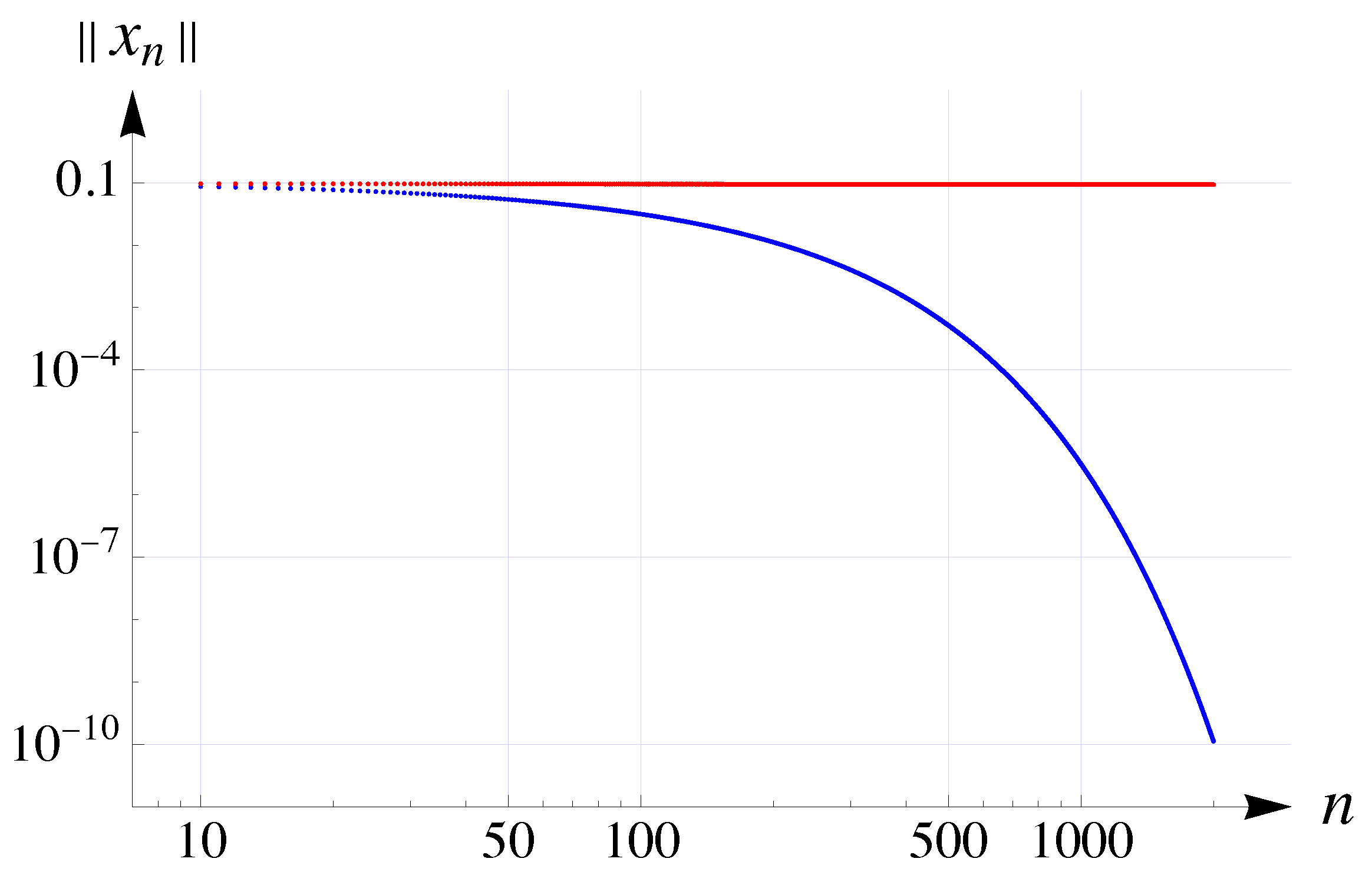
From [37] (Theorem 2.4.1, p. 167), the Fréchet derivative of f at a point $\mathit{x}$ is $\nabla f\mathit{x}=4{\mathit{x}}^3+2\mathit{x}=4{\left\{x_k^3\right\}}_{k=0}^{\infty }+2{\left\{x_k\right\}}_{k=0}^{\infty }$, which is unique. For $x_k,y_k\in [-1,1]$, we have

$$\left(4x_k^3-4y_k^3+2\left(x_k-y_k\right)\right)\left(x_k-y_k\right)\ge -{\displaystyle \frac{1}{784}}4\left(x_k^2+x_k{y}_k+y_k^2\right){\left(x_k-y_k\right)}^2+2{\left(x_k-y_k\right)}^2,$$

from which we deduce

$$\begin{array}{cc}\hfill 〈\nabla f\mathit{x}-\nabla f\mathit{y},\mathit{x}-\mathit{y}〉& =\sum _{n=0}^{\infty }\left(4x_k^3-4y_k^3+2\left(x_k-y_k\right)\right)\left(x_k-y_k\right)\hfill \\ \hfill & \ge -{\displaystyle \frac{1}{784}}{∥T\mathit{x}-T\mathit{y}∥}^2+2{∥\mathit{x}-\mathit{y}∥}^2.\hfill \end{array}$$

This means that $\nabla f$ is a relaxed $\left(1/784,2\right)$ cocoercive operator. Additionally, since

$${\parallel \nabla f\mathit{x}-\nabla f\mathit{y}\parallel }^2=\sum _{k=0}^{\infty }{\left(4x_k^3-4y_k^3+2\left(x_k-y_k\right)\right)}^2\le {14}^2{∥\mathit{x}-\mathit{y}∥}^2,$$

$\nabla f\mathit{x}$ is a 14-Lipschitz function.

Let $S:H\to H$ be defined by $S\mathit{x}=sin\mathit{x}={\left\{sin{x}_k\right\}}_{k=0}^{\infty }$. The operator S is nonexpansive since

$${∥S\mathit{x}-S\mathit{y}∥}^2=\sum _{k=0}^{\infty }2{\left|sin{\displaystyle \frac{x_k-y_k}{2}}\right|}^2{\left|cos{\displaystyle \frac{x_k+y_k}{2}}\right|}^2\le \sum _{k=0}^{\infty }{\left|x_k-y_k\right|}^2={∥\mathit{x}-\mathit{y}∥}^2.$$

Moreover, $F\left(S\right)=\left\{{\left\{0\right\}}_{k=0}^{\infty }\right\}$. Based on assumptions (12) and (44), we set $\sigma =1/392$, ${\gamma }_1=1/2$, and $r_1=1.4999995$. Consequently, we calculate $\delta =0.99616612$ and $L=0.001$, which yields $2L+\delta =0.99816612<1$. Also, we have $F\left(S\right)=\left\{{\left\{0\right\}}_{k=0}^{\infty }\right\}$. It is evident that these parameter choices satisfy conditions (12) and (44).

Next, let $a_n=b_n=c_n=1/(n+1)$ for all n. To ensure clarity, we denote a sequence of elements in the Hilbert space H as ${\left\{{\mathit{x}}_n\right\}}_{n=0}^{\infty }$, where ${\mathit{x}}_n=(x_{n,0},x_{n,1},x_{n,2},\dots )\in H$. Under these notations, the iterative algorithms defined in (43) and (11) are reformulated as follows:

$$\left.\begin{array}{c}{\mathit{x}}_0={\left\{x_{0,k}\right\}}_{k=0}^{\infty }\in H,\hfill \\ x_{n+1,k}=sin\left\{P_H\left[{\displaystyle \frac{390y_{n,k}-4{\left(y_{n,k}\right)}^3}{392}}\right]\right\},\hfill \\ y_{n,k}=\left(1-{\displaystyle \frac{1}{n+1}}\right)sin\left\{P_H\left[{\displaystyle \frac{390x_{n,k}-4{\left(x_{n,k}\right)}^3}{392}}\right]\right\}+{\displaystyle \frac{1}{n+1}}sin\left\{P_H\left[{\displaystyle \frac{390z_{n,k}-4{\left(z_{n,k}\right)}^3}{392}}\right]\right\},\hfill \\ z_{n,k}=\left(1-{\displaystyle \frac{1}{n+1}}\right)x_{n,k}+{\displaystyle \frac{1}{n+1}}sin\left\{P_H\left[{\displaystyle \frac{390x_{n,k}-4{\left(x_{n,k}\right)}^3}{392}}\right]\right\}\hfill \end{array}\right\}$$

(45)

and

$$\left.\begin{array}{c}{\mathit{x}}_0={\left\{x_{0,k}\right\}}_{k=0}^{\infty }\in H,\hfill \\ x_{n+1,k}=\left(1-{\displaystyle \frac{1}{n+1}}\right)x_{n,k}+{\displaystyle \frac{1}{n+1}}sin\left\{P_H\left[{\displaystyle \frac{390y_{n,k}-4{\left(y_{n,k}\right)}^3}{392}}\right]\right\},\hfill \\ y_{n,k}=\left(1-{\displaystyle \frac{1}{n+1}}\right)x_{n,k}+{\displaystyle \frac{1}{n+1}}sin\left\{P_H\left[{\displaystyle \frac{390z_{n,k}-4{\left(z_{n,k}\right)}^3}{392}}\right]\right\},\hfill \\ z_{n,k}=\left(1-{\displaystyle \frac{1}{n+1}}\right)x_{n,k}+{\displaystyle \frac{1}{n+1}}sin\left\{P_H\left[{\displaystyle \frac{390x_{n,k}-4{\left(x_{n,k}\right)}^3}{392}}\right]\right\},\hfill \end{array}\right\}$$

(46)

where $P_H:\mathcal{H}\to H$ is defined by $P_H\mathit{x}=\mathit{x}$, when $\mathit{x}\in H$, and $P_H\mathit{x}=\mathit{x}/\parallel \mathit{x}\parallel$, when $\mathit{x}\notin H$.

Let the initial point for both iterative processes be the sequence ${\mathit{x}}_0={\left\{1/{10}^{k+1}\right\}}_{n=0}^{\infty }\in H$. From

Table 1. Convergence behavior of algorithm (45).

n	${\mathit{x}}_{\mathit{n}}={\left\{{\mathit{x}}_{\mathit{n},\mathit{k}}\right\}}_{\mathit{k}=0}^{\mathit{\infty }}$	$∥{\mathit{x}}_{\mathit{n}}∥$
0	$\{{10}^{-1},{10}^{-2},{10}^{-3},{10}^{-4},\dots \}$	$1.0050378\times {10}^{-1}$
1	$\{9.7967792\times {10}^{-2},9.8472060\times {10}^{-3},9.8477132\times {10}^{-4},9.8477183\times {10}^{-5},\dots \}$	$9.8466417\times {10}^{-2}$
10	$\{8.6656450\times {10}^{-2},8.9532943\times {10}^{-3},8.9563123\times {10}^{-4},8.9563425\times {10}^{-5},\dots \}$	$8.7122397\times {10}^{-2}$
100	$\{3.1258552\times {10}^{-2},3.5598150\times {10}^{-3},3.5651069\times {10}^{-4},3.5651600\times {10}^{-5},\dots \}$	$3.1462641\times {10}^{-2}$
500	$\{5.1356941\times {10}^{-4},5.9449351\times {10}^{-5},5.9550580\times {10}^{-6},5.9551595\times {10}^{-7},\dots \}$	$5.1703345\times {10}^{-4}$
1000	$\{3.0841463\times {10}^{-6},3.5701370\times {10}^{-7},3.5762164\times {10}^{-8},3.5762773\times {10}^{-9},\dots \}$	$3.1049491\times {10}^{-6}$
2000	$\{1.1122794\times {10}^{-10},1.2875491\times {10}^{-11},1.2897416\times {10}^{-12},1.2897635\times {10}^{-13},\dots \}$	$1.1197818\times {10}^{-10}$
$\downarrow$	$\downarrow$	$\downarrow$
∞	${\left\{0\right\}}_{k=0}^{\infty }$	$0$

and

Table 2. Convergence behavior of algorithm (46).

n	${\mathit{x}}_{\mathit{n}}={\left\{{\mathit{x}}_{\mathit{n},\mathit{k}}\right\}}_{\mathit{k}=0}^{\mathit{\infty }}$	$∥{\mathit{x}}_{\mathit{n}}∥$
0	$\{{10}^{-1},{10}^{-2},{10}^{-3},{10}^{-4},\dots \}$	$1.0050378\times {10}^{-1}$
1	$\{9.79677792\times {10}^{-2},9.8472060\times {10}^{-3},9.8477132\times {10}^{-4},9.8477183\times {10}^{-5},\dots \}$	$9.8466417\times {10}^{-2}$
10	$\{9.6217387\times {10}^{-2},9.7133063\times {10}^{-3},9.7142348\times {10}^{-4},9.7142441\times {10}^{-5},\dots \}$	$9.6711360\times {10}^{-2}$
100	$\{9.4718081\times {10}^{-2},9.5972797\times {10}^{-3},9.5985596\times {10}^{-4},9.5985724\times {10}^{-5},\dots \}$	$9.5207948\times {10}^{-2}$
500	$\{9.3707517\times {10}^{-2},9.5183569\times {10}^{-3},9.5198684\times {10}^{-4},9.5198835\times {10}^{-5},\dots \}$	$9.4194550\times {10}^{-3}$
1000	$\{9.3277892\times {10}^{-2},9.4846274\times {10}^{-3},9.4862361\times {10}^{-4},9.4862522\times {10}^{-5},\dots \}$	$9.3763705\times {10}^{-2}$
2000	$\{9.2851285\times {10}^{-2},9.4510301\times {10}^{-3},9.4527346\times {10}^{-4},9.4527516\times {10}^{-5},\dots \}$	$9.3335876\times {10}^{-2}$
$\downarrow$	$\downarrow$	$\downarrow$
∞	${\left\{0\right\}}_{k=0}^{\infty }$	$0$

, as well as from Figure 1, it is evident that both algorithms (45) and (46) converge strongly to the point $\mathbf{0}=(0,0,0,\dots )$. Furthermore, the algorithm in (45) exhibits faster convergence compared to the algorithm in (46).

As a prototype, consider the mapping Φ, $\tilde{\Phi }:H\to H$, be defined as

$$\Phi \left(\mathit{x}\right)=sin\left\{P_H\left[{\displaystyle \frac{390x_k-4{\left(x_k\right)}^3}{392}}\right]\right\}$$

and $\tilde{\Phi }\left(\mathit{x}\right)=\tilde{\Phi }\left({\left\{x_n\right\}}_{n=0}^{\infty }\right)={\left\{x_n^3\right\}}_{n=0}^{\infty }=\left(x_0^3,x_1^3,x_2^3,x_3^3,\dots \right)$. With these definitions, the results of Theorems 4, 5, and 6 can be straightforwardly verified. All computations in this example were performed using Wolfram Mathematica 14.2.

4. Numerical Experiments

In this section, we adapt and apply the iterative algorithm (11) within the context of machine learning to demonstrate the practical significance of the theoretical results derived in this study. By doing so, we highlight the real-world applicability of the proposed methods beyond their theoretical foundations. Furthermore, we compare the performance of algorithm (11) with algorithm (10), providing additional support for the validity of the theorems presented in previous sections.

Our focus is on the framework of loss minimization in machine learning, employing two novel projected gradient algorithms to solve related optimization problems. Specifically, we consider a regression/classification setup characterized by a dataset consisting of m samples and d attributes, represented as $X\in {\mathbb{R}}^{m\times d}$, with corresponding outcomes (labels) Y$\in {\mathbb{R}}^m$. The optimization problem is formulated as follows:

$$minF\left(w\right)=\underset{w\in {\mathbb{R}}^d}{min}{\displaystyle \frac{1}{2}}{\parallel Xw-Y\parallel }_2^2.$$

Using the ${\ell }_1$-projection operator $P_H$ (onto the positive quadrant), $S=I$, $w\in {\mathbb{R}}^d$, $g=I$, and $T=\nabla F$, we define two iterative algorithms:

$$\left.\begin{array}{c}{w}_0\in H,\hfill \\ w_{n+1}=P_H\left[u_n-\sigma \nabla F{u}_n\right]\hfill \\ u_n=\left(1-b_n\right)P_H\left[w_n-\sigma \nabla F{w}_n\right]+b_n{P}_H\left[v_n-\sigma \nabla F{v}_n\right],\hfill \\ v_n=\left(1-c_n\right)w_n+c_n{P}_H\left[w_n-\sigma \nabla F{w}_n\right]\hfill \end{array}\right\}$$

(47)

and

$$\left.\begin{array}{c}{w}_0\in H,\hfill \\ w_{n+1}=\left(1-a_n\right)w_n+a_n{P}_H\left[u_n-\sigma \nabla F{u}_n\right],\hfill \\ u_n=\left(1-b_n\right)w_n+b_n{P}_H\left[v_n-\sigma \nabla F{v}_n\right],\hfill \\ v_n=\left(1-c_n\right)w_n+c_n{P}_H\left[w_n-\sigma \nabla F{w}_n\right],\hfill \end{array}\right\}$$

(48)

where ${\left\{a_n\right\}}_{n=0}^{\infty }$, ${\left\{b_n\right\}}_{n=0}^{\infty }$, and ${\left\{c_n\right\}}_{n=0}^{\infty }$$\subset [0,1]$. To compute the optimal value of the step size $\sigma$, a backtracking algorithm is employed. All numerical implementations and simulations were carried out using Matlab, Ver. R2023b.

The real-world datasets used in this study are:

+

Aligned Dataset (in Swarm Behavior): Swarm behavior refers to the collective dynamics observed in groups of entities such as birds, insects (e.g., ants), fish, or animals moving cohesively in large masses. These entities exhibit synchronized motion at the same speed and direction while avoiding mutual interference. The Aligned dataset comprises pre-classified data relevant to swarm behavior, including 24,017 instances with 2400 attributes (see https://archive.ics.uci.edu/ml/index.php (accessed on 14 February 2025)).

+

COVID-19 Dataset: COVID-19, an ongoing viral epidemic, primarily causes mild to moderate respiratory infections but can lead to severe complications, particularly in elderly individuals and those with underlying conditions such as cardiovascular disease, diabetes, chronic respiratory illnesses, and cancer. The dataset is a digitized collection of patient records detailing symptoms, medical history, and risk classifications. It is designed to facilitate predictive modeling for patient risk assessment, resource allocation, and medical device planning. This dataset includes 1,048,576 instances with 21 attributes (see https://datos.gob.mx/busca/dataset/informacion-referente-a-casos-covid-19-en-mexico (accessed on 14 February 2025)).

+

Predict Diabetes Dataset: Provided by the National Institute of Diabetes and Digestive and Kidney Diseases (USA), this dataset contains diagnostic metrics for determining the presence of diabetes. It consists of 768 instances with 9 attributes, enabling the development of predictive models for diabetes diagnosis (see https://www.kaggle.com/datasets (accessed on 14 February 2025)).

+

Sobar Dataset: The Sobar dataset focuses on factors related to cervical cancer prevention and management. It includes both personal and social determinants, such as perception, motivation, empowerment, social support, norms, attitudes, and behaviors. The dataset comprises 72 instances with 20 attributes (see https://archive.ics.uci.edu/ml/index.php (accessed on 14 February 2025)).

The methodology for dataset analysis and model evaluation was carried out as follows:

All datasets were split into training $(60\%)$ and testing $(40\%)$ subsets. During the analysis, we set the tolerance value (i.e., the difference between two successive function values) to ${10}^{-5}$ and capped the maximum number of iterations at ${10}^5$. To evaluate the performance of algorithms on these datasets, we recorded the following metrics:

• Function values $F\left(w_n\right)$;
• The norm of the difference between the optimal function value and the function values at each iteration, i.e., $∥F\left(w_n\right)-F\left(w^{\ast }\right)∥$;
• Computation times (in seconds);
• Prediction and test accuracies, measured using root mean square error (rMSE).

The results and observations are as follows:

• Function Values: In Figure 2, the function values $F\left(w_n\right)$ for the evaluated algorithms are presented.
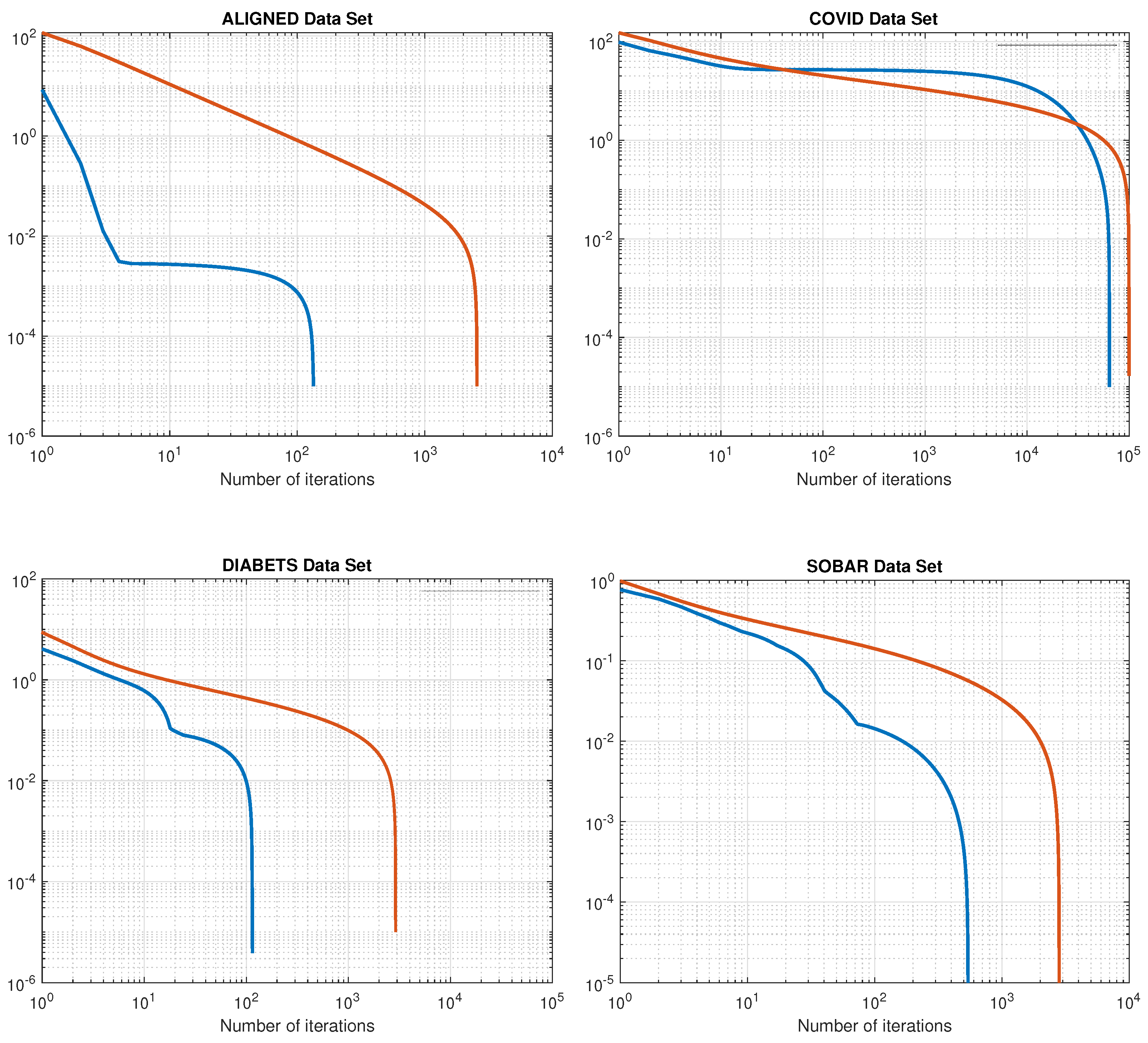
• Convergence Analysis: Figure 3 demonstrates the convergence performance of the algorithms in terms of $∥F\left(w_n\right)-F\left(w^{\ast }\right)∥$.
• Prediction Accuracy: Figure 4 show cases the prediction accuracy (rMSE) achieved by the algorithms during the testing phase.

The results, as illustrated in Figure 2, Figure 3 and Figure 4 and summarized in

Table 3. Comparison of the efficiency of algorithms (47) and (48).

	Aligned		Diabetes
	Algorithm (47)	Algorithm (48)	Algorithm (47)	Algorithm (48)
# of iterations	135	2559	116	10,480
Min F value	633.5152581	633.5407101	46.31812832	47.514786
rMse (Train.)	0.355915454	0.355922962	0.345908859	0.3504142
rMse2 (Test)	0.255097007	0.254559006	0.272919936	0.2745554
Train. time (s)	6.282856	118.1402858	0.0217341	2.8294408
	COVID-19		Sobar
	Algorithm (47)	Algorithm (48)	Algorithm (47)	Algorithm (48)
# of iterations	64,173	100,000	542	2817
Min F value	449.786	490.524	4.2837252	4.668452
rMse (Train.)	0.2994	0.3132	0.3428808	0.358791
rMse2 (Test)	0.16943	0.15862	0.288059	0.295836
Train. time (s)	187.705	420.37	0.4419386	1.013948

, clearly indicate that algorithm (47) outperforms algorithm (48) in terms of efficiency and accuracy.

Table 3 clearly demonstrates that algorithm (47) yields significantly better results than algorithm (48) across various datasets. In terms of the number of iterations, (47) converges in far fewer steps (for example, 135 versus 2559 for the Aligned dataset and 116 versus 10,480 for the Diabetes dataset) and achieves the same or lower minimum F values, resulting in superior outcomes. Moreover, (47) shows slightly lower training errors (rMse) and, in most cases—with the exception of COVID-19, where (48) achieves a marginally better test error—comparable or improved test errors (rMse2). Most importantly, the training time for (47) is significantly shorter across all datasets (for instance, 6.28 s versus 118.14 s for the Aligned dataset and 0.022 s versus 2.83 s for the Diabetes dataset), which confers an advantage in computational efficiency. Overall, these results demonstrate that algorithm (47) not only converges faster but also delivers better performance in terms of both accuracy and computational cost compared to algorithm (48).

5. Conclusions

This study presents the development of a novel Picard-S hybrid iterative algorithm designed to address general variational inequalities and nonexpansive mappings within real Hilbert spaces. By relaxing the stringent constraints traditionally imposed on parametric sequences, the proposed algorithm achieves enhanced flexibility and broader applicability while retaining its strong convergence properties. This advancement not only bridges gaps in the existing theoretical framework but also establishes a robust equivalence between the new method and a previously established algorithm, demonstrating its consistency and efficacy. One of the key contributions of this work is the integration of the Collage–Anticollage Theorem, which provides an innovative perspective on transformations associated with general nonlinear variational inequalities (GNVI). This theorem, explored for the first time in this context, enriches the theoretical toolkit for analyzing and solving variational inequalities. The study also delves into the continuity properties of solutions to variational inequalities, addressing a rarely discussed yet crucial aspect of these problems, thereby offering a more holistic approach to their resolution. Numerical experiments conducted as part of this research validate the proposed algorithm’s superior performance. In comparison to an existing algorithm, the new algorithm consistently converges to optimal solutions with fewer iterations, underscoring its computational efficiency and practical advantages. Applications in areas such as convex optimization and machine learning further highlight its versatility. For example, the algorithm has shown promise in solving real-world problems related to classification, regression, and large-scale optimization tasks, solidifying its relevance in both theoretical and applied domains.

References

1. Stampacchia, G. Formes bilinearies coercivities sur les ensembles convexes. C. R. Acad. Sci. Paris 1964, 258, 4413–4416. [Google Scholar]
2. Lions, J.; Stampacchia, G. Variational inequalities. Commun. Pure Appl. Math. 1967, 20, 493–519. [Google Scholar] [CrossRef]
3. Kinderlehrer, D.; Stampacchia, G. An Introduction to Variational Inequalities and Their Applications; Academic Press: New York, NY, USA, 1980. [Google Scholar]
4. Glowinski, R.; Lions, J.L.; Trémolières, R. Numerical Analysis of Variational Inequalities; North-Holland: Amsterdam, The Netherlands, 1981. [Google Scholar]
5. Giannessi, F.; Maugeri, A. (Eds.) Variational Inequalities and Network Equilibrium Problems; Springer: New York, NY, USA, 1995. [Google Scholar]
6. Atalan, Y.; Hacıoğlu, E.; Ertürk, M.; Gürsoy, F.; Milovanović, G.V. Novel algorithms based on forward-backward splitting technique: Effective methods for regression and classification. J. Glob. Optim. 2024, 90, 869–890. [Google Scholar] [CrossRef]
7. Gürsoy, F.; Hacıoğlu, E.; Karakaya, V.; Milovanović, G.V.; Uddin, I. Variational inequality problem involving multivalued nonexpansive mapping in CAT(0) Spaces. Results Math. 2022, 77, 131. [Google Scholar] [CrossRef]
8. Keten Çopur, A.; Hacıoğlu, E.; Gürsoy, F.; Ertürk, M. An efficient inertial type iterative algorithm to approximate the solutions of quasi variational inequalities in real Hilbert spaces. J. Sci. Comput. 2021, 89, 50. [Google Scholar] [CrossRef]
9. Gürsoy, F.; Ertürk, M.; Abbas, M. A Picard-type iterative algorithm for general variational inequalities and nonexpansive mappings. Numer. Algorithms 2020, 83, 867–883. [Google Scholar] [CrossRef]
10. Atalan, Y. On a new fixed point iterative algorithm for general variational inequalities. J. Nonlinear Convex Anal. 2019, 20, 2371–2386. [Google Scholar]
11. Maldar, S. Iterative algorithms of generalized nonexpansive mappings and monotone operators with application to convex minimization problem. Symmetry 2022, 14, 1841–1868. [Google Scholar] [CrossRef]
12. Maldar, S. New parallel fixed point algorithms and their application to a system of variational inequalities. J. Appl. Math. Comput. 2022, 68, 1025. [Google Scholar] [CrossRef]
13. Konnov, I.V. Combined relaxation methods for variational inequalities. In Lecture Notes in Mathematical Economics; Springer: Berlin/Heidelberg, Germany, 2000. [Google Scholar]
14. Facchinei, F.; Pang, J.-S. Finite Dimensional Variational Inequalities and Complementarity Problems; Springer: New York, NY, USA; Berlin/Heidelberg, Germany, 2003; Volumes I and II. [Google Scholar]
15. Giannessi, F.; Maugeri, A. (Eds.) Variational Analysis and Applications; Springer: New York, NY, USA, 2005. [Google Scholar]
16. Ansari, Q.H. (Ed.) Topics in Nonlinear Analysis and Optimization; World Education: Delhi, India, 2012. [Google Scholar]
17. Ansari, Q.H.; Lalitha, C.S.; Mehta, M. Generalized Convexity. In Nonsmooth Variational Inequalities and Nonsmooth Optimization; CRC Press: Boca Raton, FL, USA; London, UK; New York, NY, USA, 2014. [Google Scholar]
18. Noor, M.A. General variational inequalities. Appl. Math. Lett. 1988, 1, 119–122. [Google Scholar] [CrossRef]
19. Noor, M.A. Variational inequalities in physical oceanography. In Ocean Waves Engineering, Advances in Fluid Mechanics; Rahman, M., Ed.; WIT Press: Southampton, UK, 1994; Volume 2. [Google Scholar]
20. Bnouhachem, A.; Liu, Z.B. Alternating direction method for maximum entropy subject to simple constraint sets. J. Math. Anal. Appl. 2004, 121, 259–277. [Google Scholar] [CrossRef]
21. Kocvara, M.; Outrata, J.V. On implicit complementarity problems with application in mechanics. In Proceedings of the the IFIP Conference on Numerical Analysis and Optimization, Rabat, Marocco, 15–17 December 1993. [Google Scholar]
22. Noor, M.A. General variational inequalities and nonexpansive mappings. J. Math. Anal. Appl. 2007, 331, 810–822. [Google Scholar] [CrossRef]
23. Ahmad, R.; Ansari, Q.H.; Irfan, S.S. Generalized variational inclusions and generalized resolvent equations in Banach spaces. Comput. Math. Appl. 2005, 29, 1825–1835. [Google Scholar] [CrossRef]
24. Ahmad, R.; Ansari, Q.H. Generalized variational inclusions and H-resolvent equations with H-accretive operators. Taiwan. J. Math. 2007, 111, 703–716. [Google Scholar] [CrossRef]
25. Ahmad, R.; Ansari, Q.H. An iterative algorithm for generalized nonlinear variational inclusions. Appl. Math. Lett. 2000, 13, 23–26. [Google Scholar] [CrossRef]
26. Fang, Y.P.; Huang, N.J. H-Monotone operator and resolvent operator technique for variational inclusions. Appl. Math. Comput. 2003, 145, 795–803. [Google Scholar] [CrossRef]
27. Huang, N.J.; Fang, Y.P. A new class of general variational inclusions involving maximal η-monotone mappings. Publ. Math. Debrecen 2003, 62, 83–98. [Google Scholar] [CrossRef]
28. Huang, Z.; Noor, M.A. Equivalency of convergence between one-step iteration algorithm and two-step iteration algorithm of variational inclusions for H-monotone mappings. Computers Math. Appl. 2007, 53, 1567–1571. [Google Scholar] [CrossRef]
29. Noor, M.A.; Huang, Z. Some resolvent iterative methods for variational inclusions and nonexpansive mappings. Appl. Math. Comput. 2007, 194, 267–275. [Google Scholar] [CrossRef]
30. Zeng, L.C.; Guu, S.M.; Yao, J.C. Characterization of H-monotone operators with applications to variational inclusions. Comput. Math. Appl. 2005, 50, 329–337. [Google Scholar] [CrossRef]
31. Gürsoy, F.; Sahu, D.R.; Ansari, Q.H. S-iteration process for variational inclusions and its rate of convergence. J. Nonlinear Convex Anal. 2016, 17, 1753–1767. [Google Scholar]
32. Nagurney, A. Network Economics: A Variational Inequality Approach; Springer: Berlin/Heidelberg, Germany, 1999. [Google Scholar]
33. Kotsireas, I.S.; Nagurney, A.; Pardalos, P.M. (Eds.) Dynamics of Disasters–Algorithmic Approaches and Applications; Springer Optimization and Its Applications 140; Springer: Berlin/Heidelberg, Germany, 2018. [Google Scholar]
34. Fargetta, G.; Maugeri, A.; Scrimali, L. A stochastic Nash equilibrium problem for medical supply competition. J. Optim. Theory Appl. 2022, 193, 354–380. [Google Scholar] [CrossRef]
35. Qihou, L. A convergence theorem of the sequence of Ishikawa iterates for quasi-contractive mappings. J. Math. Anal. Appl. 1990, 146, 301–305. [Google Scholar] [CrossRef]
36. Weng, X. Fixed point iteration for local strictly pseudocontractive mapping. Proc. Amer. Math. Soc. 1991, 113, 727–731. [Google Scholar] [CrossRef]
37. Milovanović, G.V. Numerical Analysis and Approximation Theory—Introduction to Numerical Processes and Solving of Equations; Zavod za udžbenike: Beograd, Serbia, 2014. (In Serbian) [Google Scholar]
Figure 1. Graph in log log scale denotes the convergence behaviors of algorithms (45) (blue line) and (46) (red line) to 0 n = 0 .
Axioms 14 00288 g001
Figure 2. Comparison of the efficiency of algorithms (47) (blue line) and (48) (red line) based on reduction in function values F ( w n ) in each step.
Axioms 14 00288 g002
Figure 3. Comparison of the efficiency of algorithms (47) (blue line) and (48) (red line) based on F ( w n ) F ( w ) in each step.
Axioms 14 00288 g003
Figure 4. Comparison of the efficiency of algorithms (47) (blue line) and (48) (red line) based on rMSE in each step.
Axioms 14 00288 g004