
A Novel Approach to Some Proximal Contractions with Examples of Its Application


Abstract
1. Introduction
2. Preliminaries
- 1.
- 2.
- iff
- 3.
- 4.
- , for each
- 1.
- 2.
- 3.
- 4.
- for allThen, is termed a rectangular metric space.
- (i)
- We can write if and only if the sequence converges to a point .
- (ii)
- If the sequence satisfies the condition , then it is known to be Cauchy.
- (iii)
- If, in the rectangular metric space ʘ, every Cauchy sequence is convergent, then we call it a complete metric space, and vice versa.
- (iv)
- The uniqueness of limits is ensured for every convergent sequence in the rectangular metric space ʘ.
- (i)
- is continuous.
- (ii)
- If , then
- (iii)
- For all , .
- ()
- θ is non-decreasing.
- ()
- For every , if and only if .
- ()
- For and .
- 1.
- ;
- 2.
- ;
- 3.
- ;
- 4.
- ;
- 5.
- ;
- 6.
- .
3. Multivalued Mapping Results
4. Single-Valued Mappings Results
5. Fixed Point Results
- Case (i): If and , we take and ; then, the distance , with
- Case (ii): If both points are taken from set , then we have two cases. In the first one, we select closely situated elements, whereas, in the second case, the chosen points are more distant from each other.
- (a)
- If and , then đ and
- (b)
- If and , then and
6. Application to Equation of Motion
- for all and with .
- There is , which gives , where .
7. Conclusions
Author Contributions
Funding
Data Availability Statement
Conflicts of Interest
References
- Khan, I.; Shaheryar, M.; Din, F.U.; Ishtiaq, U.; Popa, I.L. Fixed-Point Results in Fuzzy S-Metric Space with Applications to Fractals and Satellite Web Coupling Problem. Fractal Fract. 2025, 9, 164. [Google Scholar] [CrossRef]
- Zahid, M.; Ud Din, F.; Shah, K.; Abdeljawad, T. Fuzzy fixed point approach to study the existence of solution for Volterra type integral equations using fuzzy Sehgal contraction. PLoS ONE 2024, 19, e0303642. [Google Scholar] [CrossRef] [PubMed]
- Basha, S.; Veeramani, P. Best proximity pair theorems for multi-functions with open fibres. J. Approx. Theory 2000, 103, 119–129. [Google Scholar] [CrossRef]
- Basha, S.; Veeramani, P. Best approximations and best proximity pairs. Acta Sci. Math. 1997, 63, 289–300. [Google Scholar]
- Eldred, A.A.; Veeramani, P. Existence and convergence of best proximity points. J. Math. Anal. Appl. 2006, 323, 1001–1006. [Google Scholar] [CrossRef]
- Ishtiaq, U.; Jahangeer, F.; Kattan, D.A.; Argyros, I.K. Generalized Common Best Proximity Point Results in Fuzzy Metric Spaces with Application. Symmetry 2023, 15, 1501. [Google Scholar] [CrossRef]
- Younis, M.; Ahmad, H.; Shahid, W. Best proximity points for multivalued mappings and equation of motion. J. Appl. Anal. Comp. 2024, 14, 298–316. [Google Scholar] [CrossRef]
- Komal, S.; Hussain, A.; Sultana, N.; Kumam, P. Coincidence best proximity points for Geraghty type proximal cyclic contractions. J. Math. Comp. Sci. 2018, 18, 98–114. [Google Scholar] [CrossRef]
- Jleli, M.; Samet, B. A new generalization of the Banach contraction principle. J. Inequal. Appl. 2014, 2014, 38. [Google Scholar] [CrossRef]
- Zahid, M.; Din, F.U.; Younis, M.; Ahmad, H.; Öztürk, M. Some Results on Multivalued Proximal Contractions with Application to Integral Equation. Mathematics 2024, 12, 3488. [Google Scholar] [CrossRef]
- Sametric, B.; Vetro, C.; Vetro, P. Fixed point theorem for α-ψ-contractive type mappings. Nonlinear Anal. 2012, 75, 2154–2165. [Google Scholar]
- Feng, G.; Yu, S.; Wang, T.; Zhang, Z. Discussion on the weak equivalence principle for a Schwarzschild gravitational field based on the light-clock model. Ann. Phys. 2025, 473, 169903. [Google Scholar] [CrossRef]
- Jin, Y.; Lu, G.; Sun, W. Genuine multipartite entanglement from a thermodynamic perspective. Phys. Rev. A 2024, 109, 042422. [Google Scholar] [CrossRef]
- Liu, X.; Lou, S.; Dai, W. Further results on “System identification of nonlinear state-space models”. Automatica 2023, 148, 110760. [Google Scholar] [CrossRef]
- Gao, Q.; Deng, Z.; Ju, Z.; Zhang, T. Dual-hand motion capture by using biological inspiration for bionic bimanual robot teleoperation. Cyb. Biol. Syst. 2023, 4, 52. [Google Scholar] [CrossRef]
- Hou, Q.; Li, Y.; Singh, V.P.; Sun, Z. Physics-informed neural network for diffusive wave model. J. Hydrol. 2024, 637, 131261. [Google Scholar] [CrossRef]
- Peng, L.; Liang, Y.; He, X. Transfers to Earth-Moon triangular libration points by Sun-perturbed dynamics. Adv. Space Res. 2025, 75, 2837–2855. [Google Scholar] [CrossRef]
- Shi, Q.; Sun, Y.; Saanouni, T. On the growth of Sobolev norms for Hartree equation. J. Evol. Equ. 2025, 25, 13. [Google Scholar] [CrossRef]
- Alves, S.; Babcinschi, M.; Silva, A.; Neto, D.; Fonseca, D.; Neto, P. Integrated design fabrication and control of a bioinspired multimaterial soft robotic hand. Cybor. Biol. Syst. 2023, 4, 51. [Google Scholar] [CrossRef]
- Frechet, M.M. Sur quelques points du calcul fonctionnel. Rend. Circ. Mat. Palermo 1906, 22, 1–72. [Google Scholar] [CrossRef]
- Branciari, A. A fixed point theorem of Banach-Caccioppoli type on a class of generalized metric spaces. Publ. Math. Debr. 2000, 57, 31–37. [Google Scholar] [CrossRef]
- Sankar Raj, V. A best proximity point theorem for weakly contractive non-self-mappings. Nonlinear Anal. 2011, 74, 4804–4808. [Google Scholar] [CrossRef]
- Khan, M.S.; Swaleh, M.; Sessa, S. Fixed point theorems by altering distances between the points. Bull. Aust. Math. Soc. 1984, 30, 1–9. [Google Scholar] [CrossRef]
- Rockafellar, T.R.; Wets, R.J.V. Variational Analysis; Springer: Berlin, Germany, 2005. [Google Scholar]
- Wang, B.; Wang, Z.; Song, Y.; Zong, W.; Zhang, L.; Ji, K.; Dai, Z. GA neural coordination strategy for attachment and detachment of a climbing robot inspired by gecko locomotion. Cyb. Biol. Syst. 2023, 4, 8. [Google Scholar]
- Song, Y.; Huang, G.; Yin, J.; Wang, D. Three-dimensional reconstruction of bubble geometry from single-perspective images based on ray tracing algorithm. Meas. Sci. Technol. 2025, 36, 016010. [Google Scholar] [CrossRef]
- Erhan, I.M.; Karapınar, E.; Sekulić, T. Fixed points of (ψ,ϕ) contractions on rectangular metric spaces. Fixed Point Theory Appl. 2012, 2012, 138. [Google Scholar] [CrossRef]
- Zhang, W.; Yang, X.; Lin, J.; Lin, B.; Huang, Y. Experimental and numerical study on the torsional behavior of rectangular hollow reinforced concrete columns strengthened By CFRP. Structures 2024, 70, 107690. [Google Scholar] [CrossRef]
- Xiong, F.; Wang, L.; Huang, J.; Luo, K. A Thermodynamically Consistent Phase-Field Lattice Boltzmann Method for Two-Phase Electrohydrodynamic Flows. J. Sci. Comp. 2025, 103, 34. [Google Scholar] [CrossRef]
- Kou, J.; Wang, Y.; Chen, Z.; Shi, Y.; Guo, Q. Gait Planning and Multimodal Human-Exoskeleton Cooperative Control Based on Central Pattern Generator. IEEE/ASME Tran. Mech. 2024, 1–11. [Google Scholar] [CrossRef]
- Kou, J.; Wang, Y.; Chen, Z.; Shi, Y.; Guo, Q.; Xu, M. Flexible assistance strategy of lower limb rehabilitation exoskeleton based on admittance model. Sci. China Technol. Sci. 2024, 67, 823–834. [Google Scholar] [CrossRef]

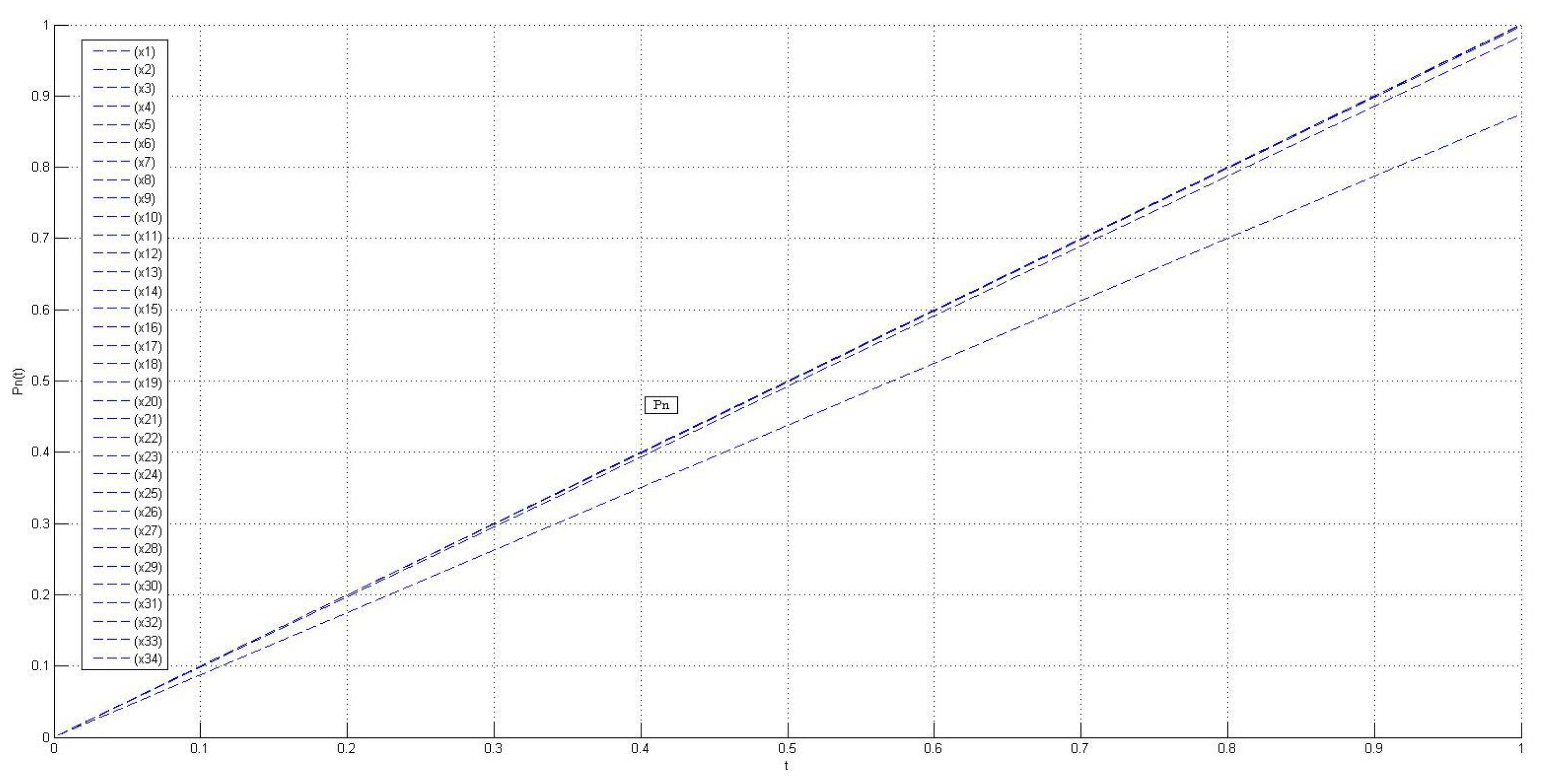
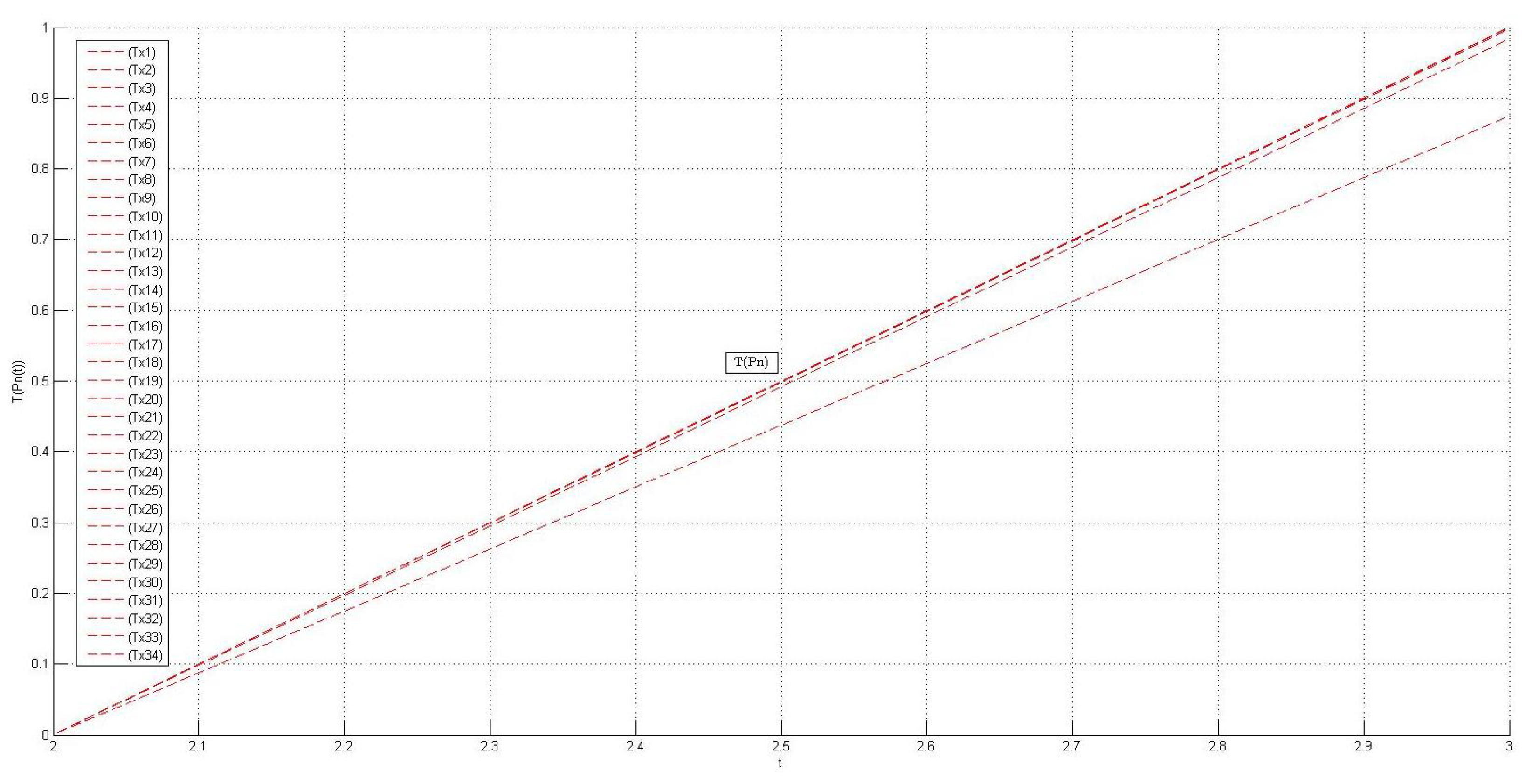
| Sr. No. | Sequence | Sequence |
|---|---|---|
| 00 | 0 | |
| 01 | ||
| 02 | ||
| 03 | ||
| 04 | ||
| 05 | ||
| 06 | ||
| 07 | ||
| 08 | ||
| 09 | ||
| 10 | ||
| ⋮ | ⋮ | ⋮ |
| 31 | ||
| 32 | ||
| 33 | ||
| 34 | ω |
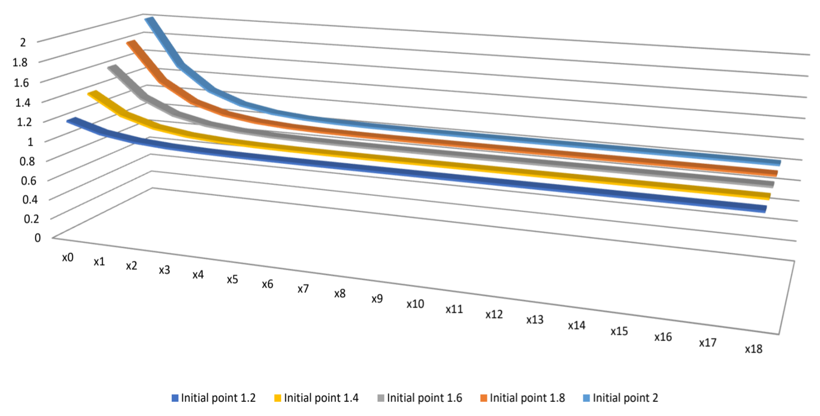
| Sr. No. | |||||
|---|---|---|---|---|---|
| 1 | 1.5 | 1.4 | 1.3 | 1.2 | 1.1 |
| 2 | 1.25 | 1.2 | 1.15 | 1.1 | 1.05 |
| 3 | 1.125 | 1.1 | 1.075 | 1.05 | 1.025 |
| 4 | 1.0625 | 1.05 | 1.0375 | 1.025 | 1.0125 |
| 5 | 1.03125 | 1.025 | 1.01875 | 1.00125 | 1.00625 |
| 6 | 1.01563 | 1.0125 | 1.00938 | 1.00625 | 1.00313 |
| 7 | 1.00781 | 1.00625 | 1.00468 | 1.00313 | 1.00157 |
| 8 | 1.00391 | 1.00313 | 1.00234 | 1.00157 | 1.00079 |
| 9 | 1.00196 | 1.00157 | 1.00117 | 1.00079 | 1.00040 |
| ⋮ | ⋮ | ⋮ | ⋮ | ⋮ | ⋮ |
| 16 | 1.00002 | 1.00001 | 1.00001 | 1 | 1 |
| 17 | 1.00001 | 1 | 1 | 1 | 1 |
| 18 | 1 | 1 | 1 | 1 | 1 |
Disclaimer/Publisher’s Note: The statements, opinions and data contained in all publications are solely those of the individual author(s) and contributor(s) and not of MDPI and/or the editor(s). MDPI and/or the editor(s) disclaim responsibility for any injury to people or property resulting from any ideas, methods, instructions or products referred to in the content. |
© 2025 by the authors. Licensee MDPI, Basel, Switzerland. This article is an open access article distributed under the terms and conditions of the Creative Commons Attribution (CC BY) license (https://creativecommons.org/licenses/by/4.0/).
Share and Cite
Zahid, M.; Din, F.U.; Cotîrlă, L.-I.; Breaz, D. A Novel Approach to Some Proximal Contractions with Examples of Its Application. Axioms 2025, 14, 382. https://doi.org/10.3390/axioms14050382
Zahid M, Din FU, Cotîrlă L-I, Breaz D. A Novel Approach to Some Proximal Contractions with Examples of Its Application. Axioms. 2025; 14(5):382. https://doi.org/10.3390/axioms14050382
Chicago/Turabian StyleZahid, Muhammad, Fahim Ud Din, Luminiţa-Ioana Cotîrlă, and Daniel Breaz. 2025. "A Novel Approach to Some Proximal Contractions with Examples of Its Application" Axioms 14, no. 5: 382. https://doi.org/10.3390/axioms14050382
APA StyleZahid, M., Din, F. U., Cotîrlă, L.-I., & Breaz, D. (2025). A Novel Approach to Some Proximal Contractions with Examples of Its Application. Axioms, 14(5), 382. https://doi.org/10.3390/axioms14050382