Article

Fractional Order Mathematical Modelling of HFMD Transmission via Caputo Derivative

by
Aakash Mohandoss
1,
Gunasundari Chandrasekar
2,*,
Mutum Zico Meetei
3,* and
Ahmed H. Msmali
3,4
1
Department of Mathematics, College of Engineering and Technology, SRM Institute of Science and Technology, Kattankulathur 603203, Tamil Nadu, India
2
Department of Mathematics, College of Engineering, Anna University, Chennai 600025, Tamil Nadu, India
3
Department of Mathematics, College of Science, Jazan University, P.O. Box 114, Jazan 45142, Saudi Arabia
4
School of Mathematics and Applied Statistics, University of Wollongong, Wollongong, NSW 2522, Australia
*
Authors to whom correspondence should be addressed.
Axioms 2024, 13(4), 213; https://doi.org/10.3390/axioms13040213
Submission received: 19 February 2024 / Revised: 13 March 2024 / Accepted: 18 March 2024 / Published: 25 March 2024
(This article belongs to the Special Issue Fractional Calculus and the Applied Analysis)

Abstract

:
This paper studies a nonlinear fractional mathematical model for hand, foot, and mouth Disease (HFMD), incorporating a vaccinated compartment. Our initial focus involves establishing the non-negativity and boundedness of the fractional order dynamical model. The existence and uniqueness of the system are discussed using the Caputo derivative operator formulation. Applying a fixed-point approach, we obtain results that confirm the presence of at least one solution. We analyze the stability behavior at the two equilibrium points (disease-free and endemic states) of the model and derive the basic reproduction number. Numerical simulations are conducted using the fractional Euler approach, and the simulation results confirm our analytical conclusions. This comprehensive approach enhances the understanding of HFMD dynamics and facilitates the policy making of health care centers to control the further spread of this disease.

1. Introduction

Mathematical modeling involves using equations or algorithms to represent real-world systems across various disciplines, such as physics, engineering, biology, economics, and social sciences. These models serve to comprehend, evaluate, and predict system behavior, playing a vital role in scientific research, engineering design, and decision-making. Mathematical modeling allows the study and control of systems in ways that are often impractical or costly in real-world experiments. The process typically includes problem formulation, model construction, parameter estimation, model validation, and model analysis. Proficiency in both system understanding and mathematics is crucial for creating and solving these equations. The validation and verification of models are essential before using them for predictions or decision-making. This interdisciplinary field combines mathematical concepts with domain-specific knowledge, providing insightful analyses of complex phenomena. Mathematical modeling is indispensable for advancing the scientific understanding, addressing real-world issues, and making well-informed decisions. Researchers, engineers, and decision-makers leverage mathematical modeling to gain knowledge, predict outcomes, and optimize systems, contributing significantly to various fields [1,2,3,4,5].
The viral illness known as hand, foot, and mouth disease (HFMD) predominantly affects children under the age of 10 and occasionally even adults. There are several enterovirus types that cause it, but Coxsackievirus A16 and Enterovirus 71 are the most frequent ones. The manifestation of diminutive and distressing blisters or ulcers on the hands, feet, and oral cavity, coupled with other indicators like fever and rash, typically points to the likelihood of hand, foot, and mouth disease (HFMD). It is highly contagious and spreads through close contact with infected individuals, contaminated surfaces, or respiratory droplets from coughs and sneezes. HFMD typically spreads in crowded places like daycare centers, schools, and playgrounds, with outbreaks frequently occurring in communities, especially during the warmer months. The symptoms of HFMD usually start with fever, a sore throat, and a general feeling of malaise. Within a day or two, small blisters will develop in the hands, feet, and mouth. These blisters may be painful and can sometimes become ulcers. Other symptoms may include loss of appetite, headaches, and, in some cases, a skin rash. Although HFMD is often a temporary disease that cures by itself within 7–10 days, it can cause discomfort and sometimes complications, especially in severe cases. Complications can include viral meningitis, encephalitis (inflammation of the brain), and, in rare cases, more serious neurological complications. Treatment for HFMD is usually supportive, focusing on relieving symptoms such as fever and discomfort. Using over-the-counter pain medicines, such as acetaminophen or ibuprofen, and practicing excellent hygiene habits, such as frequent handwashing and avoiding close contact with sick people, are essential for preventing the spread of the virus. The most important prevention is to maintain good oral hygiene and minimize contact with ill people. Vaccines for HFMD are not widely available, but some countries have developed vaccines against Enterovirus 71, which is one of the common causes of severe HFMD cases. Vaccination is a method used to prevent and control infections, which can significantly enhance the immune system [6]. The authors in [7,8] examine certain findings that could aid in the development of effective enterovirus vaccines. The authors in [9] developed a dynamic model of HFMD using the SEIQR, taking into account two optimal control strategies (treatment and vaccine). Numerical solutions were utilized to assess the efficacy of the control system in response to variations in parameters. A study in [10] examined how climate change, economic development, and the population of children affect the spread of HFMD infection. A fractional order model, incorporating constant and optimum controls, was constructed in [11] to understand the transmission dynamics of HFMD. The authors in [12] constructed a fractional order model to investigate the dynamics of HFMD that included vaccination and quarantine strategies for disease intervention. They used the fundamental reproduction number to assess the stability of the model. In addition, the model utilized an optimum control study in [13] to evaluate the effectiveness of vaccination as a control strategy. The authors of [14] introduced a fractional order model for HFMD, in which the basic reproduction number is derived using the correlation coefficient approach. The simulations were conducted to understand the infection dynamics.
Fractional differential equations (FDEs) are differential equations that incorporate non-integer order derivatives. This permits the use of fractional orders, which can be any real or complex number, in contrast to ordinary differential equations (ODEs), where the order of the derivatives is always a positive integer [15]. When a system’s behavior depends on the fractional derivatives of its variables, FDEs are an effective mathematical tool for describing a wide range of physical, biological, and engineering phenomena. In the 18th and 19th centuries, mathematicians, especially Leibniz and Riemann established the concept of fractional calculus, which is associated with non-integer order derivatives and integrals. However, because of its applications in numerous disciplines, including physics, engineering, finance, and biology, it has recently attracted new interest. FDEs have been used to simulate and analyze various intricate phenomena, including viscoelastic materials, diffusion in fractal media, electrochemical processes, and biological systems. Most of the models stated above are integer order models; however, they are unable to depict real-life difficulties because there is no non-locality impact in local differentiation. Mathematicians thus developed the idea of differentiation with non-local operators to address this issue. Researchers have demonstrated that the memory effect of fractional calculus produces more accurate results when predicting physical systems, including mathematical models [16]. In order to solve systems of differential equations of both integer and non-integer orders resulting from real-life issues, such as applications related to integrodifferential equations [17,18], mathematical epidemiology [19,20], and economic and financial [21,22], new discoveries have resulted from advances in constructing new fractional order operators, especially Caputo, Atangana–Baleanu, and Caputo–Fabrizio. A fractional order model is proposed to describe the competitive market of freelancing and its significance using the Atangana–Baleanu–Caputo type [23]. A fractional model of the within-host dynamics of SARS-CoV-2 is presented in [24] using the Caputo fractional order operator. The dynamics of COVID-19 are modeled in [25] using a new hybrid fractional order operator (a linear combination of Riemann–Lioville and Caputo). Most researchers are optimistic about the fractional order differential equation, especially in biological modeling [26]. Caputo and Fabrizio proposed a unique interpretation of the fractional operator without a single kernel [27].
In this paper, we chose hand, foot, and mouth disease as our social problem and studied a five compartmental nonlinear mathematical model. Furthermore, we extend the nonlinear ODE model into a fractional order model. Then, we theoretically proved the HFMD transmission with Caputo derivative, and simultaneously, we performed the analysis of the proposed model, which proved that our model has a unique solution with two equilibrium points, which are said to be asymptotically stable. The utilization of fractional differential equations in our approach yields precise outcomes that are important in disease modeling. Through the utilization of this approach, we successfully obtained accurate solutions for the model, which enhanced our understanding of the transmission dynamics of HFMD.
The structured of the paper is as follows: Section 2 formulates the fractional order model, followed by some essential preliminaries in Section 3. In Section 4, we addressed the system’s positivity and boundedness. Section 5 discusses the suggested model’s existence and uniqueness, followed by the qualitative analysis in Section 6. Section 7 provides instructions on utilizing the modified Euler’s method to obtain the general solution for the given system. Section 8 presented a brief discussion of our findings, followed by a conclusion.

2. Model Formulation

We consider a S V E I R , a five compartment HFMD model. The basic structure of the model comprises distinct population groups, including those that are susceptible, vaccinated, exposed, infected, and recovered. In this case, we presume that not all vaccinated people are immune to this virus and that some may be exposed to it. We also believe that people who have recovered from HFMD do not have lifetime immunity to the condition. As a result, we believe that recovered people are susceptible at a rate of α 0 , and that after recovery, some people will take vaccination and therefore enter the vaccinated compartment at a rate of α 1 . As a result of the aforesaid assumptions, a basic nonlinear mathematical model was developed as follows:
d S d t = A δ 1 S I δ 2 S E μ S z S + α 0 R , d V d t = z S δ 3 V I δ 4 V E μ V + α 1 R , d E d t = δ 1 S I + δ 2 S E + δ 3 V I + δ 4 V E η E μ E , d I d t = η E γ I μ I μ 1 I , d R d t = γ I μ R α 0 R α 1 R .
It is vital to investigate viral disease mathematical models in order to have a deeper comprehension of their assessment, presence, stability, and control. Due to the limited accuracy of conventional mathematical models in describing these diseases, FDEs were developed to effectively handle such situations. FDEs have proven to be extremely helpful in several practical applications. Also, fractional derivatives are better at modeling complex systems than regular derivatives because they can better capture memory effects, non-local behaviors, and strange diffusion. Their flexibility enables a detailed representation of phenomena in bioengineering, control systems, and other areas where past events are crucial. Unlike typical derivatives, fractional calculus considers long-term memory, proving invaluable in applications where past events strongly impact the present state. Fractional calculus is a powerful tool for dealing with complexity in a variety of different areas. It gives us a better way to describe systems whose dynamics are complicated and not in the usual way. So, fractional derivatives are better than ordinary derivatives. Therefore, the ODE model for HFMD in [28] was converted to the fractional order model by using the Caputo derivative to explore a new study in HFMD transmission..
  C D t α [ S ( t ) ] = A δ 1 S I δ 2 S E μ S z S + α 0 R ,   C D t α [ V ( t ) ] = z S δ 3 V I δ 4 V E μ V + α 1 R ,   C D t α [ E ( t ) ] = δ 1 S I + δ 2 S E + δ 3 V I + δ 4 V E η E μ E ,   C D t α [ I ( t ) ] = η E γ I μ I μ 1 I ,   C D t α [ R ( t ) ] = γ I μ R α 0 R α 1 R .
Here, 0 < α ≤ 1 and S ( 0 ) = S 0 , V ( 0 ) = V 0 , E ( 0 ) = E 0 , I ( 0 ) = I 0 , and R ( 0 ) = R 0 are the initial conditions. Table 1 contains a description of the model (2) parameters.

3. Preliminaries

In this, we present the essential definitions of fractional calculus within the context of Caputo significance.
Definition 1
 ([29]). Consider a function y ∈ C m , then   C D t α in (m −1,m) where m ∈ N is provided by the following:
  C D t α ( g ( t ) ) = 1 Γ m α 0 t ( t s ) ( m α 1 ) g ( m ) ( s ) d s .
Here,   C D t α ( g ( t ) ) g ( t ) as α tends to 1.
Definition 2
 ([29]). For α > 0, the corresponding integral of g : R + R is expressed as follows:
I t α ( g ( t ) ) = 1 Γ α 0 t ( t s ) ( α 1 ) g ( s ) d s ,
where, 0 <α< 1, t> 0.

4. Positivity and Boundedness

Here, we demonstrate the boundedness and non-negative solutions of (2).
Theorem 1.
Every solution of (2) is non-negative and bounded.
Proof. 
From [30], we define N = S + V + E + I + R and μ > 0 .
  C D t α [ N ( t ) ] + μ N ( t ) = A δ 1 S I δ 2 S E μ S z S + α 0 R + z S δ 3 V I δ 4 V E μ V + α 1 R + δ 1 S I + δ 2 S E + δ 3 V I + δ 4 V E η E μ E + η E γ I μ I μ 1 I + γ I μ R α 0 R α 1 R + μ S + μ V + μ E + μ I + μ R , = A μ 1 I , A .
By using the standard comparison theorem [31] for (2), we obtain the following:
N ( t ) N ( 0 ) E α μ ( t ) α + A ( t ) α E α , α + 1 μ ( t ) α .
where the Mittag–Leffler function is represented by E α . Using Lemma 5 and Corollary 6 stated by [31], we have the following:
N ( t ) A μ , t .
Hence, all solutions of Equation (2) are restricted to the domain Ω , as follows:
Ω = { ( S , V , E , I , R ) R + 5 | N ( t ) A μ + ϵ 0 , f o r a n ϵ 0 > 0 } .
Now, we show the solutions of (2) are positive. From the first equation of (2), we have the following:
  C D t α [ S ( t ) ] = A δ 1 S I δ 2 S E μ S z S + α 0 R , [ δ 1 I + δ 2 E + μ + z ] S , [ ( δ 1 + δ 2 ) A μ + μ + z ] S , d 1 S ,
where d 1 = ( δ 1 + δ 2 ) A μ + μ + z .
As per the traditional comparison theorem [31] and the non-negativity of the Mittag–Leffler function, we have E α , 1 ( t ) > 0 for any α ( 0 , 1 ) [32], as follows:
S S ( 0 ) E α , 1 ( d 1 t α ) S 0 .
From (2), we obtain the following:
  C D t α [ V ( t ) ] = z S δ 3 V I δ 4 V E μ V + α 1 R , [ δ 3 I + δ 4 E + μ ] V , [ ( δ 3 + δ 4 ) A μ + μ ] V , d 2 V .
where d 2 = ( δ 3 + δ 4 ) A μ + μ .
Therefore,
V V ( 0 ) E α , 1 ( d 2 t α ) V 0 .
For the third equation of (2), we obtain the following:
  C D t α [ E ( t ) ] = δ 1 S I + δ 2 S E + δ 3 V I + δ 4 V E η E μ E , [ δ 2 S δ 4 V + η + μ ] E , [ δ 2 A μ δ 4 A μ + η + μ ] E , d 3 E .
Here d 3 = δ 2 A μ δ 4 A μ + η + μ .
E E ( 0 ) E α , 1 ( d 3 t α ) E 0 .
For the fourth equation of (2), we obtain the following:
  C D t α [ I ( t ) ] = η E γ I μ I μ 1 I , [ γ + μ + μ 1 ] I , d 4 I ,
where d 4 = γ + μ + μ 1 .
I I ( 0 ) E α , 1 ( d 4 t α ) I 0 .
For the fifth equation of (2), we obtain the following:
  C D t α [ R ( t ) ] = γ I μ R α 0 R α 1 R , [ μ + α 0 + α 1 ] I , d 5 R .
where d 5 = μ + α 0 + α 1 .
Therefore,
R R ( 0 ) E α , 1 ( d 5 t α ) R 0 .
Thus, the solutions of (2) are positive. □

5. Existence and Uniqueness

This section demonstrates the existence and uniqueness of the fractional order system model. We adopt a similar approach as used in [33,34]. After utilizing Equation (2), we have the following equations:
S ( t ) = S ( 0 ) +   C I 0 α S ( t ) { A δ 1 S I δ 2 S E μ S z S + α 0 R } , V ( t ) = V ( 0 ) +   C I 0 α V ( t ) { z S δ 3 V I δ 4 V E μ V + α 1 R } , E ( t ) = E ( 0 ) +   C I 0 α E ( t ) { δ 1 S I + δ 2 S E + δ 3 V I + δ 4 V E η E μ E } , I ( t ) = I ( 0 ) +   C I 0 α I ( t ) { η E γ I μ I μ 1 I } , R ( t ) = R ( 0 ) +   C I 0 α R ( t ) { γ I μ R α 0 R α 1 R } .
By using Definition 2,
S ( t ) = S ( 0 ) + 1 Γ ( α ) 0 t ( t σ ) α 1 K 1 ( σ , S , V , E , I , R ) d σ , V ( t ) = V ( 0 ) + 1 Γ ( α ) 0 t ( t σ ) α 1 K 2 ( σ , S , V , E , I , R ) d σ , E ( t ) = E ( 0 ) + 1 Γ ( α ) 0 t ( t σ ) α 1 K 3 ( σ , S , V , E , I , R ) d σ , I ( t ) = I ( 0 ) + 1 Γ ( α ) 0 t ( t σ ) α 1 K 4 ( σ , S , V , E , I , R ) d σ , R ( t ) = R ( 0 ) + 1 Γ ( α ) 0 t ( t σ ) α 1 K 5 ( σ , S , V , E , I , R ) d σ .
We defined the kernels in (18) as follows:
K 1 ( σ , S , V , E , I , R ) = A δ 1 S I δ 2 S E μ S z S + α 0 R , K 2 ( σ , S , V , E , I , R ) = z S δ 3 V I δ 4 V E μ V + α 1 R , K 3 ( σ , S , V , E , I , R ) = δ 1 S I + δ 2 S E + δ 3 V I + δ 4 V E η E μ E , K 4 ( σ , S , V , E , I , R ) = η E γ I μ I μ 1 I , K 5 ( σ , S , V , E , I , R ) = γ I μ R α 0 R α 1 R .
Assume all population groups are positive bounded function; that is, there exist some positive constants Π 1 , Π 2 , Π 3 , Π 4 , Π 5 , such that
S ( t ) Π 1 , V ( t ) Π 2 , E ( t ) Π 3 , I ( t ) Π 4 , R ( t ) Π 5 , 0 t < .
Theorem 2.
If 0 M = m a x { Δ 1 , Δ 2 , Δ 3 , Δ 4 , Δ 5 } < 1 , where Δ 1 = δ 1 Π 4 + δ 2 Π 3 + μ + z , Δ 2 = δ 3 Π 4 + δ 4 Π 3 + μ , Δ 3 = δ 2 Π 1 δ 4 Π 2 + μ + η , Δ 4 = γ + μ + μ 1 , and Δ 5 = μ + α 0 + α , then K i for i = 1 , 2 , 3 , 4 , 5 satisfies Lipschitz’s conditions.
Proof. 
Consider K 1 , for any S and S 1 ,
K 1 ( t , S , V , E , I , R ) K 1 ( t , S 1 , V , E , I , R ) = δ 1 I S δ 2 E S μ S z S + δ 1 I S 1 + δ 2 E S 1 + μ S 1 + z S 1 , = δ 1 I ( S 1 S ) + δ 2 E ( S 1 S ) + μ ( S 1 S ) + z ( S 1 S ) , δ 1 I ( t ) + δ 2 E ( t ) + μ + z S 1 S , Δ 1 S S 1 ,
where Δ 1 = δ 1 Π 4 + δ 2 Π 3 + μ + z . Thus, K 1 satisfy the Lipschitz condition. Similarly, we can find Δ j for j = 2 , 3 , 4 , 5 . Under the condition 0 M = max { Δ 1 , Δ 2 , Δ 3 , Δ 4 , Δ 5 } < 1 , the K i for i = 2 , 3 , 4 , 5 meet the Lipschitz’s requirements and are contractions. □
Now, we rewrite (18) recursively as follows:
S n ( t ) = 1 Γ ( α ) 0 t ( t σ ) α 1 K 1 ( σ , S n 1 , V n 1 , E n 1 , I n 1 , R n 1 ) d σ , V n ( t ) = 1 Γ ( α ) 0 t ( t σ ) α 1 K 2 ( σ , S n 1 , V n 1 , E n 1 , I n 1 , R n 1 ) d σ , E n ( t ) = 1 Γ ( α ) 0 t ( t σ ) α 1 K 3 ( σ , S n 1 , V n 1 , E n 1 , I n 1 , R n 1 ) d σ , I n ( t ) = 1 Γ ( α ) 0 t ( t σ ) α 1 K 4 ( σ , S n 1 , V n 1 , E n 1 , I n 1 , R n 1 ) d σ , R n ( t ) = 1 Γ ( α ) 0 t ( t σ ) α 1 K 5 ( σ , S n 1 , V n 1 , E n 1 , I n 1 , R n 1 ) d σ .
The difference between two terms can be represented as follows:
Λ n ( t ) = S n ( t ) S n 1 ( t ) = 1 Γ ( α ) 0 t ( t σ ) α 1 [ K 1 ( σ , S n 1 , V n 1 , E n 1 , I n 1 , R n 1 ) K 1 ( σ , S n 2 , V n 2 , E n 2 , I n 2 , R n 2 ) ] d σ , Ω n ( t ) = V n ( t ) V n 1 ( t ) = 1 Γ ( α ) 0 t ( t σ ) α 1 [ K 2 ( σ , S n 1 , V n 1 , E n 1 , I n 1 , R n 1 ) K 2 ( σ , S n 2 , V n 2 , E n 2 , I n 2 , R n 2 ) ] d σ , χ n ( t ) = E n ( t ) E n 1 ( t ) = 1 Γ ( α ) 0 t ( t σ ) α 1 [ K 3 ( σ , S n 1 , V n 1 , E n 1 , I n 1 , R n 1 ) K 3 ( σ , S n 2 , V n 2 , E n 2 , I n 2 , R n 2 ) ] d σ , ψ n ( t ) = I n ( t ) I n 1 ( t ) = 1 Γ ( α ) 0 t ( t σ ) α 1 [ K 4 ( σ , S n 1 , V n 1 , E n 1 , I n 1 , R n 1 ) K 4 ( σ , S n 2 , V n 2 , E n 2 , I n 2 , R n 2 ) ] d σ , ϑ n ( t ) = R n ( t ) R n 1 ( t ) = 1 Γ ( α ) 0 t ( t σ ) α 1 [ K 5 ( σ , S n 1 , V n 1 , E n 1 , I n 1 , R n 1 ) K 5 ( σ , S n 2 , V n 2 , E n 2 , I n 2 , R n 2 ) ] d σ .
where,
S n ( t ) = i = 0 n Λ i ( t ) , V n ( t ) = i = 0 n Ω i ( t ) , E n ( t ) = i = 0 n χ i ( t ) , I n ( t ) = i = 0 n ψ i ( t ) , R n ( t ) = i = 0 n ϑ i ( t ) .
Now consider the following:
Λ n ( t ) = S n ( t ) S n 1 ( t ) = 1 Γ ( α ) 0 t ( t σ ) α 1 [ K 1 ( σ , S n 1 , V n 1 , E n 1 , I n 1 , R n 1 ) K 1 ( σ , S n 2 , V n 2 , E n 2 , I n 2 , R n 2 ) ] d σ = Δ 1 Γ ( α ) 0 t S n 1 S n 2 d σ = Δ 1 Γ ( α ) 0 t Λ n 1 ( t ) d σ .
Similarly, we obtain
Ω n ( t ) = Δ 2 Γ ( α ) 0 t Ω n 1 ( t ) d σ , χ n ( t ) = Δ 3 Γ ( α ) 0 t χ n 1 ( t ) d σ , ψ n ( t ) = Δ 4 Γ ( α ) 0 t ψ n 1 ( t ) d σ , ϑ n ( t ) = Δ 5 Γ ( α ) 0 t ϑ n 1 ( t ) d σ .
Theorem 3.
(i) The functions stated in (24) exists and are smooth, (ii) If there exists t 0 > 1 such that Δ i Γ ( α ) t 0 strictly less than one for i = 1 , 2 , 3 , 4 , 5 , then at least one solution of the system exists.
Proof. 
(i) Since all populations are bounded and for each K i , where i = 1 , 2 , 3 , 4 , 5 satisfy Lipschitz’s conditions, we will obtain the following relation:
Λ n ( t ) S ( 0 ) Δ 1 Γ ( α ) t n , Ω n ( t ) V ( 0 ) Δ 2 Γ ( α ) t n , χ n ( t ) E ( 0 ) Δ 3 Γ ( α ) t n , ψ n ( t ) I ( 0 ) Δ 4 Γ ( α ) t n , ϑ n ( t ) R ( 0 ) Δ 5 Γ ( α ) t n .
Therefore, Equation (27) shows the existence and smoothness of all populations, which were defined in (24).
(ii) Here we show that S n , V n , E n , I n and R n converge to solutions of (2). Now let u n * ,   w n * ,   x n * ,   y n * ,   z n * , are remainder terms after n iterations, such that
S S ( 0 ) = S n u n * , V V ( 0 ) = V n w n * , E E ( 0 ) = E n x n * , I I ( 0 ) = I n y n * , R R ( 0 ) = R n z n * .
By using triangle inequality along with K 1 , we obtain the following:
u n * ( t ) = 1 Γ ( α ) 0 t ( t σ ) α 1 [ K 1 ( σ , S , V , E , I , R ) K 1 ( σ , S n 1 , V n 1 , E n 1 , I n 1 , R n 1 ) ] d σ Δ 1 Γ ( α ) S S n 1 t .
Iteratively using the preceding approach yields the following equation below:
u n * ( t ) Δ 1 Γ ( α ) t n + 1 Π 1 .
Then, at t 0 , we have the following:
u n * ( t ) Δ 1 Γ ( α ) t 0 n + 1 Π 1 .
Taking limit as n ,
lim n u n * ( t ) lim n Δ 1 Γ ( α ) t 0 n + 1 Π 1 .
Using hypothesis, Δ 1 Γ ( α ) t 0 < 1 . Equation (32) becomes the following:
lim n u n * ( t ) = 0 .
As n , we obtain the following:
w n * ( t ) 0 , x n * ( t ) 0 , y n * ( t ) 0 , z n * ( t ) 0 .
Thus, the system has at least one solution. □
Theorem 4.
A unique solution exists for (2) if 1 Δ i Γ ( α ) t > 0 for i = 1 to 5 .
Proof. 
Let S 1 ( t ) , V 1 ( t ) , E 1 ( t ) , I 1 ( t ) , R 1 ( t ) is another set of solution to (2) thus,
S ( t ) S 1 ( t ) = 1 Γ ( α ) 0 t ( t σ ) α 1 K 1 ( s , S , V , E , I , R ) K 1 ( s , S 1 , V 1 , E 1 , I 1 , R 1 ) d s Δ 1 Γ ( α ) t S ( t ) S 1 ( t ) .
By rearranging the following:
S ( t ) S 1 ( t ) Δ 1 Γ ( α ) t S ( t ) S 1 ( t ) 0 ,
S ( t ) S 1 ( t ) 1 Δ 1 Γ ( α ) t 0 .
Using hypothesis, if 1 Δ 1 Γ ( α ) t is strictly greater than zero, then (37) takes the structure S ( t ) S 1 ( t ) = 0 .
It means that S ( t ) = S 1 ( t ) .
By repeating the similar procedure for each solution for i = 2 , 3 , 4 , 5 , we obtain the following:
V ( t ) = V 1 ( t ) , E ( t ) = E 1 ( t ) , I ( t ) = I 1 ( t ) , R ( t ) = R 1 ( t ) .

6. Model Analysis

This section examines the existence of equilibrium points and the local stability of the system.

6.1. Equilibrium Points

In our case, we found the following two equilibrium points: E 0 = ( S 0 , V 0 , E 0 , I 0 , R 0 ) and E 1 = ( S * , V * , E * , I * , R * ) . We obtain the disease-free equilibrium point for the system (2) as E 0 = ( A θ 1 , z A θ 1 μ 0, 0, 0). Also for endemic equilibrium E 1 , we obtain S * = η A θ 4 + α 0 γ η I * θ 4 ( η θ 1 + δ 1 η I * + δ 2 θ 3 η I * ) , V * = η z θ 4 ( η A θ 4 + α 0 γ η I * θ 4 ( η θ 1 + δ 1 η I * + δ 2 θ 3 η I * ) + η α 1 γ I * ) θ 4 ( δ 3 η I * + δ 4 θ 3 I * + η μ ) , E * = θ 3 I * η , and R * = γ I * θ 4 . Here, I * will be in the form of g ( I * ) = l 1 I * 3 + l 2 I * 2 + l 3 I * + l 4 = 0 . By using the Descartes rule of signs [28], we can find the positive roots of I * .

6.2. Basic Reproduction Number (BRN)

The spectral radius of the next generation matrix determines the R 0 [5] for the system (2). Therefore, we have R 0 = η S δ 1 + η V δ 3 + S δ 2 θ 3 + θ 3 V δ 4 θ 2 θ 3 . By substituting disease-free equilibrium points we obtain the following:
R 0 = η ( A θ 1 ) δ 1 + η ( z A θ 1 μ ) δ 3 + ( A θ 1 ) δ 2 θ 3 + θ 3 ( z A θ 1 μ ) δ 4 θ 2 θ 3 .
where, θ 1 = μ + z , θ 2 = η + μ , and θ 3 = γ + μ + μ 1 .

6.3. Local Stability

The Jacobian matrix for (2) is presented by the following:
J = δ 1 I δ 2 E θ 1 0 δ 2 S δ 1 S α 0 z δ 3 I δ 4 E μ δ 4 V δ 3 V α 1 δ 1 I + δ 2 E δ 3 I + δ 4 E δ 2 S + δ 4 V θ 2 δ 3 V + δ 1 S 0 0 0 η θ 3 0 0 0 0 γ θ 4 .
Theorem 5.
The disease-free equilibrium point E 0 of the fractional order model (2) is stable if R 0 < 1 .
Proof. 
According to Matignon’s condition in [35], the E 0 of the system (2) is locally asymptotically stable if, and only if, all the eigenvalues of J 0 satisfy |arg( λ i )| > a π 2 .
The Jacobi matrix at E 0 is obtained as follows:
J 0 = θ 1 0 δ 2 A θ 1 δ 1 A θ 1 α 0 z μ δ 4 z A θ 1 μ δ 3 z A θ 1 μ α 1 0 0 δ 2 A θ 1 + δ 4 z A θ 1 μ θ 2 δ 3 z A θ 1 μ + δ 1 A θ 1 0 0 0 η θ 3 0 0 0 0 γ θ 4 .
Clearly, from the above matrix, we can say λ 1 = θ 1 , λ 2 = μ , λ 5 = θ 4 are the three eigenvalues. We can compute λ 3 and λ 4 from the following matrix:
δ 2 A θ 1 + δ 4 z A θ 1 μ θ 2 δ 3 z A θ 1 μ + δ 1 A θ 1 η θ 3 .
We have λ 3 = y 1 + y 2 + y 3 and λ 4 = y 1 y 2 + y 3 , where
y 1 = A δ 2 μ θ 1 θ 2 μ θ 1 θ 3 μ + A δ 4 z , y 2 = A 2 δ 2 2 μ 2 + θ 1 2 θ 2 2 μ 2 + 2 θ 1 2 θ 2 θ 3 μ 2 + θ 1 2 θ 3 2 μ 2 + 2 A 2 δ 2 δ 4 μ z + A 2 δ 4 2 z 2 2 A δ 2 θ 1 θ 2 μ 2 2 A δ 2 θ 1 θ 3 μ 2 2 A δ 4 θ 1 θ 2 μ z 2 A δ 4 θ 1 θ 3 μ z , y 3 = 4 ( A δ 2 θ 1 θ 3 μ 2 + δ 1 A θ 1 η μ 2 + A δ 4 θ 1 θ 3 μ z + A δ 3 θ 1 η μ z θ 1 2 θ 2 θ 3 μ 2 ) .
And,
y 1 < 0 when θ 1 θ 2 μ + θ 1 θ 3 μ > A δ 2 μ + A δ 4 z , y 2 > 0 when A 2 δ 2 2 μ 2 + θ 1 2 θ 2 2 μ 2 + 2 θ 1 2 θ 2 θ 3 μ 2 + θ 1 2 θ 3 2 μ 2 + 2 A 2 δ 2 δ 4 μ z + A 2 δ 4 2 z 2 > 2 A δ 2 θ 1 θ 2 μ 2 + 2 A δ 2 θ 1 θ 3 μ 2 + 2 A δ 4 θ 1 θ 2 μ z + 2 A δ 4 θ 1 θ 3 μ z , y 3 > 0 when 4 ( A δ 2 θ 1 θ 3 μ 2 + δ 1 A θ 1 η μ 2 + A δ 4 θ 1 θ 3 μ z + A δ 3 θ 1 η μ z ) > 4 θ 1 2 θ 2 θ 3 μ 2 .
Therefore λ 3 and λ 4 have negative real numbers with the above conditions. Table 2, shows the conditions for the stability of the equilibrium point. From this clearly, we can conclude that all eigenvalues are negative and do fulfill the Matignon’s condition [35]. Hence, E 0 = ( A θ 1 , z A θ 1 μ 0, 0, 0) is stable whenever BRN is less than one. □
Theorem 6.
When R 0 > 1 , the endemic equilibrium E 1 of the model (2) is an asymptotically stable point.
Proof. 
By using [35], the endemic equilibrium E 1 of (2) is locally asymptotically stable if, and only if, all the eigenvalues of the matrix mentioned below satisfy the condition |arg( λ i )| > a π 2 .
The Jacobi matrix at E 1 for system (2) is as follows:
J 1 = δ 1 I * δ 2 E * θ 1 0 δ 2 S * δ 1 S * α 0 z δ 3 I * δ 4 E * μ δ 4 V * δ 3 V * α 1 δ 1 I * + δ 2 E * δ 3 I * + δ 4 E * δ 2 S * + δ 4 V * θ 2 δ 3 V * + δ 1 S * 0 0 0 η θ 3 0 0 0 0 γ θ 4 .
Let us consider the following:
  • b 11 = δ 1 I * δ 2 E * θ 1 , b 13 = δ 2 S * , b 14 = δ 1 S * , b 15 = α 0 , b 21 = z ,
  • b 22 = δ 3 I * δ 4 E * μ , b 23 = δ 4 V * , b 24 = δ 3 V * , b 25 = α 1 , b 31 = δ 1 I * + δ 2 E * ,
  • b 32 = δ 3 I * + δ 4 E * , b 33 = δ 2 S * + δ 4 V * θ 2 , b 34 = δ 3 V * + δ 1 S * , b 43 = η , b 44 = θ 3 ,
  • b 54 = γ , b 55 = θ 4 .
The characteristic equation of the J 1 is as follows:
λ 5 + x 1 λ 4 + x 2 λ 3 + x 3 λ 2 + x 4 λ + x 5 = 0 ,
where,
x 1 = b 11 b 22 b 33 b 44 b 55 , x 2 = b 44 b 55 + b 33 b 55 + b 22 b 55 + b 11 b 55 + b 33 b 44 + b 22 b 44 + b 11 b 44 + b 22 b 33 + b 11 b 33 + b 11 b 22 b 34 b 43 b 23 b 32 b 13 b 31 , x 3 = b 34 b 43 b 55 + b 23 b 32 b 55 + b 13 b 31 b 55 + b 23 b 32 b 44 + b 13 b 31 b 44 + b 22 b 34 b 43 + b 11 b 34 b 43 + b 11 b 23 b 32 + b 13 b 22 b 31 b 33 b 44 b 55 b 22 b 44 b 55 b 11 b 44 b 55 b 22 b 33 b 55 b 11 b 33 b 55 b 11 b 22 b 55 b 22 b 33 b 44 b 11 b 33 b 44 b 11 b 22 b 44 b 24 b 32 b 43 b 14 b 31 b 43 b 11 b 22 b 33 b 13 b 21 b 32 , x 4 = b 22 b 33 b 44 b 55 + b 11 b 33 b 44 b 55 + b 11 b 22 b 44 b 55 + b 24 b 32 b 43 b 55 + b 14 b 31 b 43 b 55 + b 11 b 22 b 33 b 55 + b 13 b 21 b 32 b 55 + b 11 b 22 b 33 b 44 + b 11 b 23 b 32 b 44 + b 13 b 21 b 32 b 44 + b 11 b 24 b 32 b 43 + b 14 b 22 b 31 b 43 b 23 b 32 b 44 b 55 b 13 b 31 b 44 b 55 b 22 b 34 b 43 b 55 b 11 b 34 b 43 b 55 b 11 b 23 b 32 b 55 b 13 b 22 b 31 b 55 b 25 b 32 b 43 b 54 b 15 b 31 b 43 b 54 b 13 b 22 b 31 b 44 b 1 b 22 b 34 b 43 b 14 b 21 b 32 b 43 , x 5 = b 11 b 23 b 32 b 44 b 55 + b 13 b 22 b 31 b 44 b 55 + b 11 b 22 b 34 b 43 b 55 + b 14 b 21 b 32 b 43 b 55 + b 11 b 25 b 32 b 43 b 54 + b 15 b 22 b 31 b 43 b 54 b 11 b 22 b 33 b 44 b 55 b 13 b 21 b 32 b 44 b 55 b 11 b 24 b 32 b 43 b 55 b 14 b 22 b 31 b 43 b 55 b 15 b 21 b 32 b 43 b 54 .
Now, we have
x 1 > 0 , if b 11 + b 22 + b 33 + b 44 + b 55 < 0 , x 2 > 0 , if b 11 b 33 + b 11 b 22 > b 34 b 43 + b 23 b 32 + b 13 b 31 , x 3 > 0 , if b 11 b 34 b 43 + b 11 b 23 b 32 + b 13 b 22 b 31 > b 33 b 44 b 55 + b 22 b 44 b 55 + b 11 b 44 b 55 + b 22 b 33 b 55 + b 11 b 33 b 55 + b 11 b 22 b 55 + b 22 b 33 b 44 + b 11 b 33 b 44 + b 11 b 22 b 44 + b 24 b 32 b 43 + b 14 b 31 b 43 + b 11 b 22 b 33 + b 13 b 21 b 32 , x 4 > 0 , if b 11 b 24 b 32 b 43 + b 14 b 22 b 31 b 43 > b 23 b 32 b 44 b 55 + b 13 b 31 b 44 b 55 + b 22 b 34 b 43 b 55 + b 11 b 34 b 43 b 55 + b 11 b 23 b 32 b 55 + b 13 b 22 b 31 b 55 + b 25 b 32 b 43 b 54 + b 15 b 31 b 43 b 54 + b 13 b 22 b 31 b 44 + b 1 b 22 b 34 b 43 + b 14 b 21 b 32 b 43 , x 5 > 0 , if b 11 b 23 b 32 b 44 b 55 > b 11 b 22 b 33 b 44 b 55 + b 13 b 21 b 32 b 44 b 55 + b 11 b 24 b 32 b 43 b 55 + b 14 b 22 b 31 b 43 b 55 + b 15 b 21 b 32 b 43 b 54 .
From the above conditions, we can say that, E 1 = ( S * , E * , I * , Q * , R * , D * ) of Equation (2) is stable whenever R 0 > 1 . □

7. Numerical Simulation

In this, we derive the general fractional order Euler method approach for (2). By reformulating, we obtain the following:
D t α [ S ( t ) ] = τ 1 ( t , S ( t ) ) , D t α [ V ( t ) ] = τ 2 ( t , V ( t ) ) , D t α [ E ( t ) ] = τ 3 ( t , E ( t ) ) , D t α [ I ( t ) ] = τ 4 ( t , I ( t ) ) , D t α [ R ( t ) ] = τ 5 ( t , R ( t ) ) .
where,
τ 1 ( t , S ( t ) ) = A δ 1 S I δ 2 S E μ S z S + α 0 R , τ 2 ( t , V ( t ) ) = z S δ 3 V I δ 4 V E μ V + α 1 R , τ 3 ( t , E ( t ) ) = δ 1 S I + δ 2 S E + δ 3 V I + δ 4 V E η E μ E , τ 4 ( t , I ( t ) ) = η E γ I μ I μ 1 I , τ 5 ( t , R ( t ) ) = γ I μ R α 0 R α 1 R .
From the first equation of (2),
D t α [ S ( t ) ] = τ 1 ( t , S ( t ) ) , S ( 0 ) = S 0 , t > 0 .
Figure 1, shows the simulation of the SVEIR model at both the disease-free and endemic equilibrium points, considering the basic reproduction numbers. The local stability of the SVEIR model for disease-free and endemic equilibrium is illustrated in Figure 1a,b, respectively. Figure 1a emphasize the model behavior at the disease-free equilibrium point. This equilibrium point signifies a scenario where the spread of the disease is halted and individuals return to a non-infected state. In this context, basic reproduction numbers, which are critical in epidemiology, are taken into account. The local stability of the system is explored, visualizing how small perturbations affect the equilibrium. The plot provides insights into how the model behaves under disease-free conditions, taking into account the impact of basic reproduction numbers on equilibrium stability. In Figure 1b, the focus shifts to the endemic equilibrium point, representing a scenario where the disease persists in the population. Basic reproduction numbers, similar to Figure 1a, significantly influence the local stability of the system. The plot provides a visual representation of the equilibrium points concerning the endemic state. This allows for an understanding of the stability of the system when the disease is present and continues to circulate throughout the population. The model simulation provides a concise representation of the epidemic’s dynamics within a limited timeframe, namely, when time t ranges from 0 to 20 days and vaccination is implemented among the population. As time progresses, the rate at which people get vaccinated has an impact on the trajectory of illness within the community. Our proposed model exhibits a greater efficacy in forecasting the disease’s behavior within a limited timeframe. Since the model has a fractional order, it can be adjusted in order to more accurately match the actual data based on the progressions.
Let [ 0 , d ] be the collection of points for which we wish to find the solution of (51). In fact, we are unable to assess S ( t ) that will correspond to (51). We form a collection of ( t r , t r + 1 ) and these points in our iterative approach. From t r = r h , r = 0 , 1 , 2 , 3 , k , we partition the interval [ 0 , d ] into k subintervals [ t r , t r + 1 ] with equal width h = d k . Assume S ( t ) , D t α [ S ( t ) ] , and D t 2 α [ S ( t ) ] are continuous on [ 0 , d ] . By using the generalized Taylor formula, extend S ( t ) to t = t 0 = 0 . There is a value c 1 for each value t, therefore
S ( t ) = S ( t 0 ) + D t α [ S ( t ) ] t 0 t α Γ ( α + 1 ) + D t 2 α [ S ( t ) ] c 1 t 2 α Γ ( 2 α + 1 ) .
Substitute D t α [ S ( t ) ] t 0 = τ 1 ( t 0 , S ( t 0 ) ) and h = t 1 in (52), yield the following:
S ( t 1 ) = S ( t 0 ) + τ 1 ( t 0 , S ( t 0 ) ) h α Γ ( α + 1 ) + D t 2 α [ S ( t ) ] c 1 h 2 α Γ ( 2 α + 1 ) .
If h is small, thus the following:
S ( t 1 ) = S ( t 0 ) + τ 1 ( t 0 , S ( t 0 ) ) h α Γ ( α + 1 ) .
A general formula, t r + 1 = t r + h can be written as follows:
S ( t r + 1 ) = S ( t r ) + τ 1 ( t r , S ( t r ) ) h α Γ ( α + 1 ) .
Using the fractional integral on (51), we obtain the following:
[ S ( t ) ] = S ( 0 ) + I α [ τ 1 ( t , S ( t ) ) ] .
To obtain ( t 1 , S ( t 1 ) ) , we replace t = t 1 into (56), then
S ( t 1 ) = S ( 0 ) + ( I α [ τ 1 ( t , S ( t ) ) ] ) ( t 1 ) .
With the help of the modified trapezoidal rule, we approximate ( I α [ τ 1 ( t , S ( t ) ) ] ) ( t 1 ) with h = t 1 t 0 then (57) becomes the following
S ( t 1 ) = S ( 0 ) + α h α [ τ 1 ( t 0 , S ( t 0 ) ) ] Γ ( α + 2 ) + h α [ τ 1 ( t 1 , S ( t 1 ) ) ] Γ ( α + 2 ) .
The expression S ( t 1 ) appears in the formula on the RHS of (58). As a result, we estimate S ( t 1 ) . For this purpose, the fractional Euler approach is used. Substitute (54) for (58).
S ( t 1 ) = S ( 0 ) + α h α [ τ 1 ( t 0 , S ( t 0 ) ) ] Γ ( α + 2 ) + h α [ τ 1 ( t 1 , S ( t 0 ) ) ] + h α Γ ( α + 1 ) τ 1 ( t 0 , S ( t 0 ) ) Γ ( α + 2 ) .
The technique is iterated until a sequence of points that closely approximates the solution is obtained. Thus, we can express the general formula for our approach as follows:
S ( t r ) = S ( 0 ) + h α Γ ( α + 2 ) [ ( r 1 ) α + 1 ( r α 1 ) r α ] τ 1 ( t 0 , S ( t 0 ) ) + h α Γ ( α + 2 ) i = 1 r 1 [ ( r i + 1 ) α + 1 2 ( r 1 ) α + 1 + ( r i 1 ) α + 1 ] τ 1 ( t i , S ( t i ) ) + h α Γ ( α + 2 ) τ 1 [ t r , S ( t r 1 ) + h α Γ ( α + 1 ) τ 1 ( t r 1 , S ( t r 1 ) ) ] .
Using the same method, we construct numerical schemes for the model’s additional compartments.
V ( t r ) = V ( 0 ) + h α Γ ( α + 2 ) [ ( r 1 ) α + 1 ( r α 1 ) r α ] τ 2 ( t 0 , V ( t 0 ) ) + h α Γ ( α + 2 ) i = 1 r 1 [ ( r i + 1 ) α + 1 2 ( r 1 ) α + 1 + ( r i 1 ) α + 1 ] τ 2 ( t i , V ( t i ) ) + h α Γ ( α + 2 ) τ 2 [ t r , V ( t r 1 ) + h α Γ ( α + 1 ) τ 2 ( t r 1 , V ( t r 1 ) ) ] ,
E ( t r ) = E ( 0 ) + h α Γ ( α + 2 ) [ ( r 1 ) α + 1 ( r α 1 ) r α ] τ 3 ( t 0 , E ( t 0 ) ) + h α Γ ( α + 2 ) i = 1 r 1 [ ( r i + 1 ) α + 1 2 ( r 1 ) α + 1 + ( r i 1 ) α + 1 ] τ 3 ( t i , E ( t i ) ) + h α Γ ( α + 2 ) τ 3 [ t r , E ( t r 1 ) + h α Γ ( α + 1 ) τ 3 ( t r 1 , E ( t r 1 ) ) ] ,
I ( t r ) = I ( 0 ) + h α Γ ( α + 2 ) [ ( r 1 ) α + 1 ( r α 1 ) r α ] τ 4 ( t 0 , I ( t 0 ) ) + h α Γ ( α + 2 ) i = 1 r 1 [ ( r i + 1 ) α + 1 2 ( r 1 ) α + 1 + ( r i 1 ) α + 1 ] τ 4 ( t i , I ( t i ) ) + h α Γ ( α + 2 ) τ 4 [ t r , I ( t r 1 ) + h α Γ ( α + 1 ) τ 4 ( t r 1 , I ( t r 1 ) ) ] ,
R ( t r ) = R ( 0 ) + h α Γ ( α + 2 ) [ ( r 1 ) α + 1 ( r α 1 ) r α ] τ 5 ( t 0 , R ( t 0 ) ) + h α Γ ( α + 2 ) i = 1 r 1 [ ( r i + 1 ) α + 1 2 ( r 1 ) α + 1 + ( r i 1 ) α + 1 ] τ 5 ( t i , R ( t i ) ) + h α Γ ( α + 2 ) τ 5 [ t r , R ( t r 1 ) + h α Γ ( α + 1 ) τ 5 ( t r 1 , R ( t r 1 ) ) ] .
The aforementioned numerical scheme is used to obtain the numerical simulations of the model. In order to simplify the calculations, we assume the initial states of variables and input parameters.
Let us consider the following: A = 1000 , δ 1 = 0.0009 , δ 2 = 0.0008 , δ 3 = 0.009 , δ 4 = 0.0008 , μ = 0.9 , μ 1 = 0.042 , z = 0.099 , α 0 = 0.05 , α 1 = 0.005 , γ = 0.0052 , and η = 0.7 . Using this set of parameter values, we obtain the following:
R 0 = η ( A θ 1 ) δ 1 + η ( z A θ 1 μ ) δ 3 + ( A θ 1 ) δ 2 θ 3 + θ 3 ( z A θ 1 μ ) δ 4 θ 2 θ 3 , = 0.945 < 1 .
Thus, we are able to conclude that the disease-free equilibrium E 0 is locally stable. Subsequently, after that, we make some small changes in the parameter value. Again, using these change values in the parameter, we obtain the following:
R 0 = η ( A θ 1 ) δ 1 + η ( z A θ 1 μ ) δ 3 + ( A θ 1 ) δ 2 θ 3 + θ 3 ( z A θ 1 μ ) δ 4 θ 2 θ 3 , = 1.738 > 1 .
which is illustrated in Figure 1b. Thus, we demonstrate that the endemic equilibrium E 1 is locally stable.
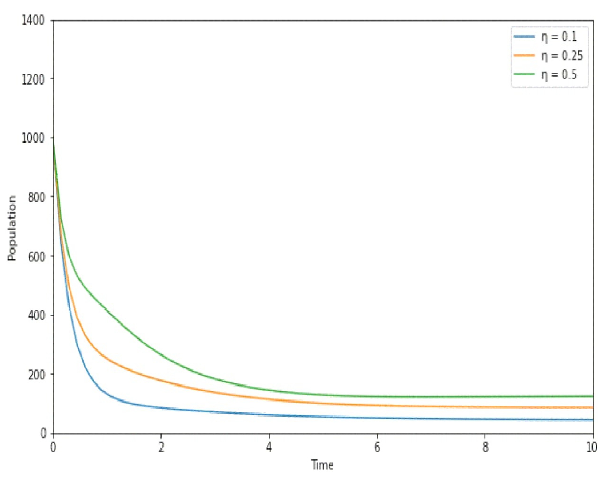
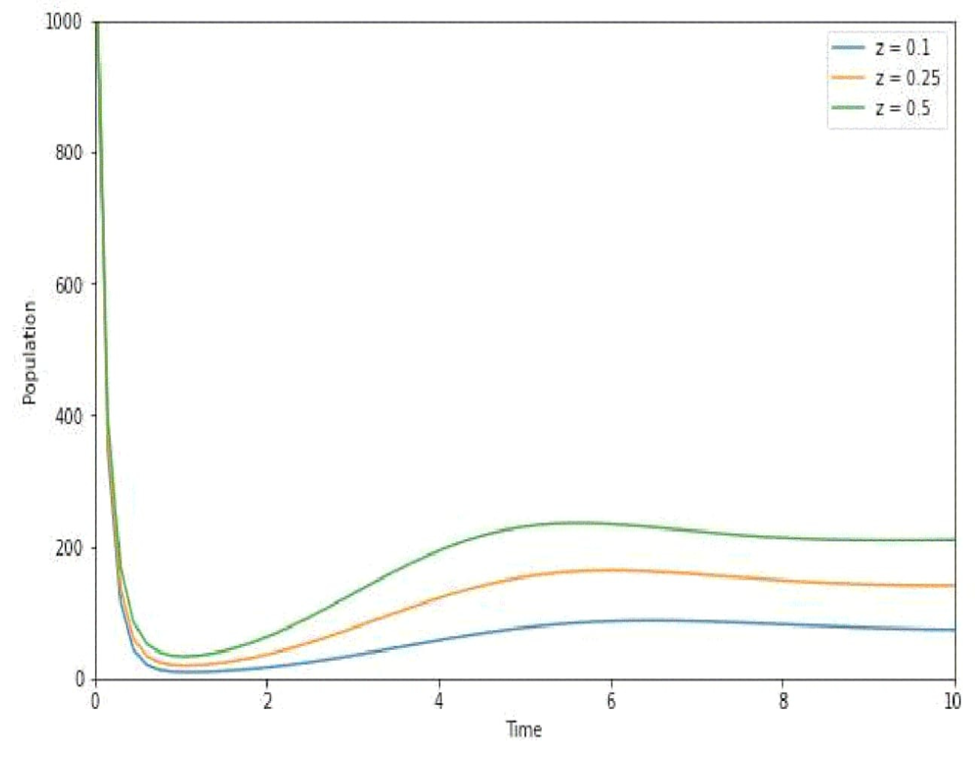
Figure 2, Figure 3 and Figure 4 display the outcomes of the most efficient instances of dynamic behavior among the infected, recovered, and vaccinated individuals at different rates. These figures represent the influence of the rate of progression for infected, recovered, and vaccinated people, respectively. Figure 5a,b shows the phase diagram for the vaccinated, infected, and recovered populations of both disease-free and endemic equilibrium DFE and EE.
In this simulation, we explore the impact of a varying progression rate ( η ), recovery rate ( γ ), and vaccination rate parameter (z) on the dynamics of an infectious disease model. We set the progression rate η at the following three different levels: 0.10, 0.25, and 0.50. As η represents the transition rate from the exposed to the infected class, an increase in its value leads to a gradual rise in the number of infected individuals, a trend visually represented in the simulation results. Furthermore, we investigate the influence of the recovery rate γ , which denotes the rate at which individuals recover due to treatment. For this analysis, we consider the following three recovery rate values: 0.10, 0.25, and 0.50. Notably, as the recovery rate γ increases, there is a pronounced surge in the number of recovered individuals, as depicted in Figure 4. Similarly, we examine the scenario for another parameter (rate of vaccination), z, and observe analogous trends. The outcomes of this investigation are graphically illustrated in the corresponding Figure 5, specifically showing the dynamic behavior of vaccinated individuals with various rates of vaccination. This comprehensive analysis reveals the intricate interplay of input parameters η , γ , and z in shaping the output dynamics of our system. The graphical representation provides a clear visualization of how changes in these key parameters impact the simulated progression of the infectious disease model, offering valuable insights into the system’s behavior under different conditions.

8. Discussion

This section discusses the practical significance of the results and their potential implications for disease control and prevention strategies.
  • Improved Understanding of Transmission Dynamics: The proposed fractional order mathematical model enhanced the understanding of the transmission dynamics of HFMD. By utilizing non-integer derivatives, the model may capture more accurately the complex and memory-dependent aspects of disease spread. This improved understanding is fundamental for designing targeted control strategies;
  • Predictive Capabilities for Outbreaks: This model contributes to the development of more accurate predictive tools for HFMD outbreaks. By considering non-local interactions and historical data more effectively, the model could provide better forecasts, enabling authorities to prepare for and respond to potential outbreaks more proactively;
  • Assessing the Impact of Control Measures: The model’s ability to capture the intricacies of HFMD transmission can be valuable in assessing the impact of implemented control measures. This feedback loop is crucial for evaluating the effectiveness of interventions and refining strategies as needed to enhance overall disease control efforts;
  • Informing Vaccination Policies: Fractional order modeling may assist in informing vaccination policies by providing a more nuanced understanding of how vaccination efforts impact disease transmission. This could aid in optimizing vaccination coverage, determining the most effective age groups for vaccination, and adapting strategies in response to changing epidemiological trends;
  • Resource Allocation and Public Health Planning: A more accurate representation of HFMD transmission dynamics can contribute to better resource allocation and planning. Health agencies can use the model to identify high-risk areas or populations, allocate resources strategically, and plan interventions in a way that maximizes their impact on disease prevention.
The Caputo fractional order mathematical modeling methodology, together with its accompanying methodologies, holds great potential for future applications in various domains, including epidemiology and ecology. The utilization of these advanced modeling tools has the capacity to make a substantial impact across multiple areas. Potential applications encompass the creation of forecasting models for emerging infectious diseases, providing understanding of their dynamics, and assisting in proactive public health interventions. Moreover, these techniques can have a crucial impact on improving vaccination regimens, guiding strong public health policies, and understanding the complex dynamics of ecological systems. As these techniques progress, their use in these and other domains is ready to completely change our understanding and response to intricate difficulties in the fields of health, environment, and beyond.

9. Conclusions

In this study, we focus on investigating the applicability of the CFO mathematical model to understanding the spread dynamics of hand, foot, and mouth disease (HFMD). The focus of our investigation is to determine whether the system is non-negative and bounded, which allowed us to analyze the stability of the model. Through nonlinear analysis, we demonstrated the existence and uniqueness of the model, which enhanced its reliability in predicting disease spread. Furthermore, we calculated the numerical solution of the suggested system using the fractional Euler’s approach. This approach is widely used to solve fractional differential equations, and it provides accurate results that are vital in disease modeling. By utilizing this method, we were able to obtain precise solutions for the model, which allowed us to make better predictions about HFMD’s transmission. Overall, our study demonstrates that the Caputo fractional order mathematical model is a reliable tool for understanding the spread of HFMD. The establishment of positive invariance and boundedness of the system, coupled with the use of nonlinear analysis and numerical solutions, enhances the accuracy of the model, which can be used to inform policies aimed at controlling and preventing the spread of HFMD. The future development of this approach holds promise for even greater contributions to the field of infectious disease modeling. The utilization of advanced computational techniques and evolving mathematical methodologies could further refine the accuracy and efficiency of the Caputo fractional order model. Additionally, the incorporation of real-time data and the consideration of more complex factors, such as spatial dynamics and demographic variations, could enhance the model’s predictive capabilities. These advancements would not only enrich our understanding of HFMD transmission, but also contribute to a more robust and adaptable tool for public health policymakers.

Author Contributions

Conceptualization, A.M. and G.C.; methodology, A.M., G.C. and M.Z.M.; software, A.H.M.; validation, A.M. and A.H.M.; formal analysis, A.M. and G.C.; investigation, A.M.; resources, A.M. and A.H.M.; data curation, A.H.M.; writing—original draft preparation, A.M., G.C. and M.Z.M.; writing—review and editing, A.M. and A.H.M.; visualization, A.M. and M.Z.M.; supervision, G.C. and A.H.M.; project administration, M.Z.M.; funding acquisition, M.Z.M. All authors have read and agreed to the published version of the manuscript.

Funding

This research was funded by the Deputyship for Research and Innovation, Ministry of Education in Saudi Arabia ISP-2024.

Data Availability Statement

Data are contained within the article.

Acknowledgments

The authors extend their appreciation to the Deputyship for Research and Innovation, Ministry of Education in Saudi Arabia, for funding this research work through the project number ISP-2024.

Conflicts of Interest

The authors declare no conflicts of interest.

References

  1. Santhosh Kumar, G.; Gunasundari, C. Turing instability of a Diffusive Predator-Prey Model along with an Allee Effect on a Predator. Commun. Math. Biol. Neurosci. 2022, 40, 1–15. [Google Scholar]
  2. Sharmila, N.B.; Gunasundari, C. Travelling Wave Solutions for a Diffusive Prey-Predator Model with One Predator and Two Preys. Int. J. Appl. Math. 2022, 35, 661. [Google Scholar] [CrossRef]
  3. Ahmadini, A.H.A.; Hassan, A.S.; Zaky, A.N.; Alshqaq, S.S. Bayesian inference of dynamic cumulative residual entropy from Pareto II distribution with application to COVID-19. AIMS Math. 2020, 6, 2196–2216. [Google Scholar] [CrossRef]
  4. Aakash, M.; Gunasundari, C.; Al-Mdallal, Q.M. Mathematical modeling and simulation of SEIR model for COVID-19 outbreak: A case study of Trivandrum. Front. Appl. Math. Stat. 2023, 9, 1124897. [Google Scholar]
  5. Aakash, M.; Gunasundari, C. Effect of Partially and Fully Vaccinated Individuals in some Regions of India: A Mathematical Study on COVID-19 Outbreak. Commun. Math. Biol. Neurosci. 2023, 2023, 25. [Google Scholar]
  6. Sivakumar, S.; Moni, S.I.A.; Aamena, J.; Mohammed, E.E.; Duaa, A.; Gassem, G.; Bassem, O.; Abdulla, M.F.; Ahmed, A.J.; Mahdi, M.A.; et al. Advancements in Vaccine Adjuvants: The Journey from Alum to Nano Formulations. Vaccines 2023, 11, 1704. [Google Scholar]
  7. Abdulaziz, A.; Famara, S.; Mouna, L.; Magloire, P.N.; Francis, B.B.; Ilka, E.; Enagnon, K.A.; Didier, H. Enteroviruses and Type 1 Diabetes Mellitus: An Overlooked Relationship in Some Regions. Microorganisms 2020, 8, 1458. [Google Scholar]
  8. Syed, Z.S.; Basit, J.; Muhammad, U.M.; Muhammad, W.; Shahkaar, A.; Sobia, A.H.; Amjad, A.; Shazia, R.; Muhammad, I.; Asaad, K.; et al. An Immunoinformatics Approach to Design a Potent Multi-Epitope Vaccine against Asia-1 Genotype of Crimean-Congo Haemorrhagic Fever Virus Using the Structural Glycoproteins as a Target. Vaccines 2023, 11, 61. [Google Scholar]
  9. Wongvanich, N.; Tang, I.-M.; Dubois, M.-A.; Pongsumpun, P. Mathematical Modeling and Optimal Control of the Hand Foot Mouth Disease Affected by Regional Residency in Thailand. Mathematics 2021, 9, 2863. [Google Scholar] [CrossRef]
  10. Sun, J.; Wu, S.; Yan, Z.; Li, Y.; Yan, C.; Zhang, F.; Liu, R.; Du, Z. Using geographically weighted regression to study the seasonal influence of potential risk factors on the incidence of HFMD on the Chinese mainland. ISPRS Int. J. Geo-Inf. 2021, 10, 448. [Google Scholar] [CrossRef]
  11. Shi, R.; Lu, T. Dynamic analysis and optimal control of a fractional order model for hand-foot-mouth disease. J. Appl. Math. Comput. 2020, 64, 565–590. [Google Scholar] [CrossRef]
  12. Gashirai, T.B.; Hove-Musekwa, S.D.; Mushayabasa, S. Dynamical analysis of a fractional-order foot-and-mouth disease model. Math. Sci. 2021, 15, 65–82. [Google Scholar] [CrossRef]
  13. Gashirai, T.B.; Hov-Musekwa, S.D.; Mushayabasa, S. Optimal control applied to a fractional-order foot-and-mouth disease model. Int. J. Appl. Comput. Math. 2021, 7, 73. [Google Scholar] [CrossRef]
  14. Rashid, J.; Boulaaras, S.; Alyobi, S.; Jawad, M. Transmission dynamics of Hand–Foot–Mouth Disease with partial immunity through non-integer derivative. Int. J. Biomath. 2023, 16, 2250115. [Google Scholar]
  15. Rao, S.N.; Alesemi, M. On a coupled system of fractional differential equations with nonlocal non-separated boundary conditions. Adv. Differ. Equ. 2019, 2019, 97. [Google Scholar] [CrossRef]
  16. Li, X.P.; DarAssi, M.H.; Khan, M.A.; Chukwu, C.W.; Mohammad, Y.A.; Mesfer, A.S.; Muhammad, B.R. Assessing the potential impact of COVID-19 Omicron variant: Insight through a fractional piecewise model. Results Phys. 2022, 38, 105652. [Google Scholar] [CrossRef] [PubMed]
  17. Kumar, P.R.; Haloi, R.; Bahuguna, D.; Dwijendra, N.P. Existence of solutions to a new class of abstract non-instantaneous impulsive fractional integro-differential equations. Nonlinear Dyn. Syst. Theory. 2016, 16, 73–85. [Google Scholar]
  18. Atangana, A.; Baleanu, D. New fractional derivatives with nonlocal and non-singular kernel: Theory and application to heat transfer model. Therm Sci. 2016, 20, 763–769. [Google Scholar] [CrossRef]
  19. Fatmawati; Shaiful, E.M.; Utoyo, M.I. A fractional-order model for HIV dynamics in a two-sex population. Int. J. Math. Math. Sci. 2018, 2018, 763–769. [Google Scholar]
  20. Bonyah, E.; Zarin, R.; Fatmawati, E.M. Mathematical modeling of cancer and hepatitis co-dynamics with non-local and non-singular kernel. Commun. Math. Biol. Neurosci. 2020.
  21. Tarasova, V.V.; Tarasov, V.E. Comments on the article long and short memory in economics: Fractional-order difference and differentiation. Probl. Mod. Sci. Educ. 2017, 31, 26–28. [Google Scholar] [CrossRef]
  22. Wang, W.; Khan, M.A.; Fatmawati; Kumam, P.; Thounthong, P. A Comparison study of bank data in fractional calculus. Chaos Solitons Fractals 2019, 126, 369–384. [Google Scholar] [CrossRef]
  23. Khan, F.S.; Khalid, M.; Al-moneef, A.; Ali, A.H.; Bazighifan, O. Freelance Model with Atangana–Baleanu Caputo Fractional Derivative. Symmetry 2022, 14, 2424. [Google Scholar] [CrossRef]
  24. Haq, I.U.; Yavuz, M.; Ali, N.; Akgül, A. A SARS-CoV-2 Fractional-Order Mathematical Model via the Modified Euler Method. Math. Comput. Appl. 2022, 27, 82. [Google Scholar] [CrossRef]
  25. Sweilam, N.H.; AL-Mekhlafi, S.M.; Hassan, S.M.; Alsenaideh, N.R.; Radwan, A.E. New Coronavirus (2019-nCov) Mathematical Model Using Piecewise Hybrid Fractional Order Derivatives; Numerical Treatments. Mathematics 2022, 10, 4579. [Google Scholar] [CrossRef]
  26. Sharmila, N.B.; Gunasundari, C. Stability Analysis of a Fractional Order Prey-Predator Model with Disease in Preys. Math. Appl. 2022, 50, 287–302. [Google Scholar]
  27. Nortey, S.N.; Juga, M.; Bonyah, E. Fractional order modelling of Anthrax-Listeriosis coinfection with nonsingular Mittag Leffler law. Sci. Afr. 2022, 16, 287–302. [Google Scholar] [CrossRef]
  28. Aakash, M.; Gunasundari, C.; Rashid, J. Modelling and Analysis of Vaccination Effects on Hand, Foot, and Mouth Disease Transmission Dynamics. Math. Model. Eng. Probl. 2023, 6, 1937–1949. [Google Scholar]
  29. Ramesh, P.; Sambath, M.; Mohd Hafiz, M.; Krishnan, B. Stability analysis of the fractional-order prey-predator model with infection. Int. J. Model. Simul. 2020, 41, 434–450. [Google Scholar] [CrossRef]
  30. Belgaid, Y.; Helal, M.; Lakmeche, A.; Venturino, E. Mathematical Study of a Coronavirus Model with the Caputo Fractional-Order Derivative. Fractal Fract. 2021, 5, 87. [Google Scholar] [CrossRef]
  31. Choi, S.K.; Kang, B.; Koo, N. Stability for Caputo fractional differential systems. Abstr. Appl. Anal. 2014, 2014, 631419. [Google Scholar] [CrossRef]
  32. Wei, Z.; Li, Q.; Che, J. Initial value problems for fractional differential equations involving Riemann-Liouville sequential fractional derivative. J. Math. Anal. Appl. 2010, 367, 260–272. [Google Scholar] [CrossRef]
  33. Ahmad, S.; Ullah, A.; Al-Mdallal, Q.; Khan, H.; Shah, K.; Khan, A. Fractional order mathematical modeling of COVID-19 transmission. Chaos Solitons Fractals 2020, 139, 110256. [Google Scholar] [CrossRef]
  34. Arshad, S.; Siddique, I.; Nawaz, F.; Shaheen, A.; Khurshid, H. Dynamics of a fractional order mathematical model for COVID-19 epidemic transmission. Phys. A Stat. Mech. Its Appl. 2023, 609, 128383. [Google Scholar] [CrossRef]
  35. Askar, S.S.; Ghosh, D.; Santra, P.K.; Elsadany, A.A.; Mahapatra, G.S. A fractional order SITR mathematical model for forecasting of transmission of COVID-19 of India with lockdown effect. Results Phys. 2021, 24, 104067. [Google Scholar] [CrossRef] [PubMed]
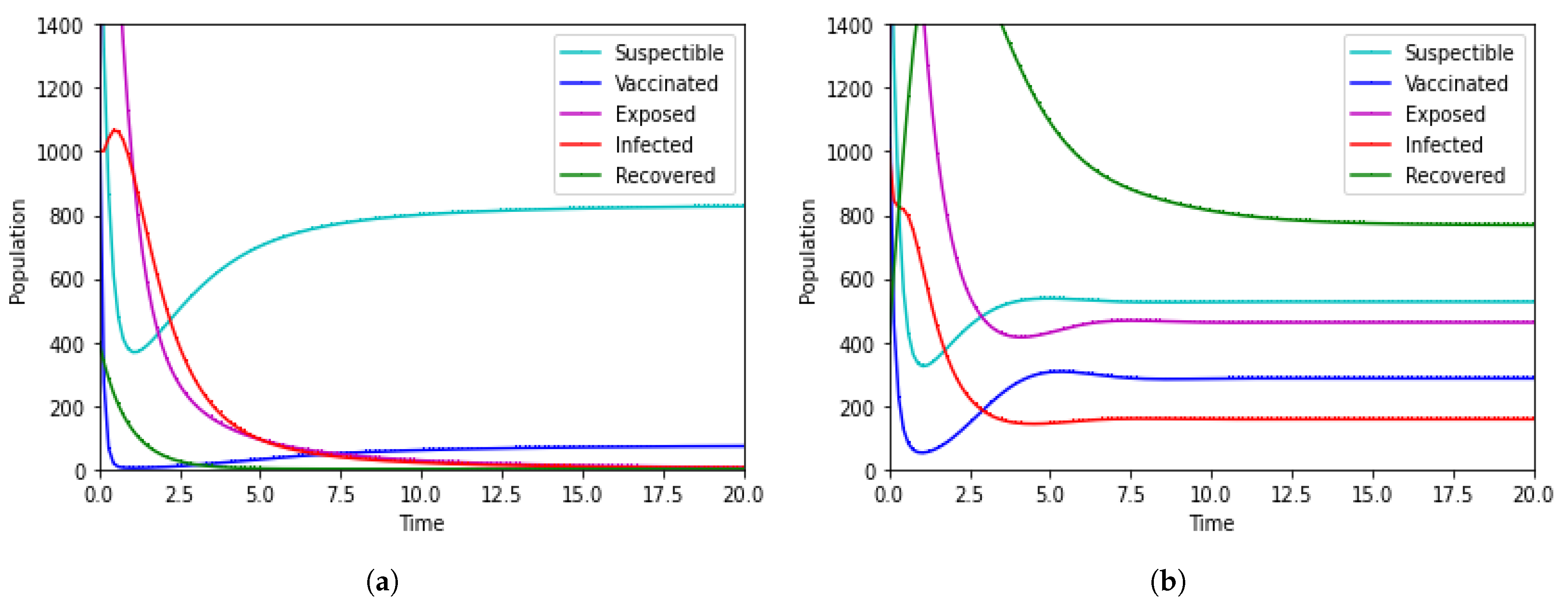
Figure 1. Phase diagram of simulation for the SVEIR model at (a) BRN = 0.945 and (b) BRN = 1.738, respectively.
Axioms 13 00213 g001
Figure 2. Dynamical behavior of infected individuals at various infected rates.
Axioms 13 00213 g002
Figure 3. Dynamical behavior of recovered individuals at various recovered rates.
Axioms 13 00213 g003
Figure 4. Dynamical behavior of vaccinated individuals at various vaccinated rates.
Axioms 13 00213 g004
Figure 5. 3D phase diagram of V, I, R for corresponding (a) E 0 and (b) E 1 .
Axioms 13 00213 g005
Table 1. Overview of the parameters.
ParametersDescription
ARate of recruitment.
δ 1 Rate of transmission from I to S.
δ 2 Rate of transmission from E to S.
δ 3 Rate of transmission from infected to vaccinated.
δ 4 Rate of transmission from exposed to vaccinated.
μ Natural death rate.
α 1 Transmission from recovered to vaccinated.
η Rate of progression from exposed to infected.
γ Rate of recovery.
μ 1 Death due to HFMD disease.
α 0 Rate from recovered to susceptible.
zRate of vaccination [28].
Table 2. Necessary components for the stability of the equilibrium point.
EigenvaluesSignConditionsStability
λ 3 y 1 < 0 , y 2 > 0 , and y 3 > 0 , and hence y 1 > y 2 + y 3 Stable
λ 4 y 1 < 0 , y 2 > 0 , and y 3 > 0 , and hence y 1 y 2 + y 3 < 0 Stable
Disclaimer/Publisher’s Note: The statements, opinions and data contained in all publications are solely those of the individual author(s) and contributor(s) and not of MDPI and/or the editor(s). MDPI and/or the editor(s) disclaim responsibility for any injury to people or property resulting from any ideas, methods, instructions or products referred to in the content.