Construction of Fractional Pseudospectral Differentiation Matrices with Applications

Abstract

Differentiation matrices are an important tool in the implementation of the spectral collocation method to solve various types of problems involving differential operators. Fractional differentiation of Jacobi orthogonal polynomials can be expressed explicitly through Jacobi–Jacobi transformations between two indexes. In the current paper, an algorithm is presented to construct a fractional differentiation matrix with a matrix representation for Riemann–Liouville, Caputo and Riesz derivatives, which makes the computation stable and efficient. Applications of the fractional differentiation matrix with the spectral collocation method to various problems, including fractional eigenvalue problems and fractional ordinary and partial differential equations, are presented to show the effectiveness of the presented method.

1. Introduction

A differentiation matrix plays a key role in implementing the spectral collocation method (also known as the pseudospectral method) to obtain numerical solutions to problems such as partial differential equations. The efficient computation of the differentiation matrix of integer order is discussed in [1,2,3,4,5] and a Matlab suite is introduced in [6].

During the past several decades, the theory and applications of fractional calculus have developed rapidly [7,8,9,10,11]. Researchers note that fractional calculus has broad and significant application prospects [8,12,13,14]. Numerous differential equation models that involve fractional calculus operators, referring to fractional differential equations, have emerged in various areas, including physics, chemistry, engineering and even finance and the social sciences.

Publications devoted to numerical solutions to fractional differential equations are numerous. Among them, the spectral collocation method is highlighted as one of the most important numerical methods. Zayernouri et al. [15] studied fractional spectral collocation methods for linear and nonlinear variable-order fractional partial differential equations. Jiao et al. [16] suggested fractional collocation methods using a fractional Birkhoff interpolation basis for fractional initial and boundary value problems. Dabiri et al. [17] presented a modified Chebyshev differentiation matrix and utilized it to solve fractional differential equations. Al-Mdallal et al. [18] presented a fractional-order Legendre collocation method to solve fractional initial value problems. Gholami et al. [19] derived a new pseudospectral integration matrix to solve fractional differential equations. Wu et al. [20] applied fractional differentiation matrices in solving Caputo fractional differential equations. Moreover, the spectral collocation method has been applied to solve tempered fractional differential equations [21,22,23], variable-order Fokker–Planck equations [24] and Caputo–Hadamard fractional differential equations [25].

The spectral collocation method approximates the unknown solution to fractional differential equations with classical orthogonal polynomials and equates the numerical solution at collocation points (usually Gauss-type quadrature nodes). Fractional differentiation in physical space is performed by the differentiation matrix as a discrete version of its continuous fractional derivative operator. Therefore, a crucial step to implement the spectral collocation method is to form the differentiation matrix. One way to construct a fractional differentiation matrix for the spectral collocation method is based on the following formula of Jacobi polynomials (see Equation (3.96) of p. 71, [26])

$$P_n^{\alpha ,\beta }\left(x\right)=\sum _{k=0}^n\frac{\mathsf{\Gamma }(n+\alpha +1)\mathsf{\Gamma }(n+k+\alpha +\beta +1)}{k!(n-k)!\mathsf{\Gamma }(k+\alpha +1)\mathsf{\Gamma }(n+\alpha +\beta +1)}{\left(\frac{x-1}{2}\right)}^k,$$

which suffers from the roundoff error [27,28]. Another way is based on the well-known three-term recurrence relationship of Jacobi polynomials (Equation (7) in next section), which gives a fast and stable evaluation of a fractional differentiation matrix [29]. Similar recurrence relationships are derived to evaluate the differentiation matrix [21,23,24,25] for various problems. In addition, there is little research on efficiently evaluating the fractional collocation differentiation matrix.

The key point in implementing the spectral collocation method is to stably and efficiently evaluate the collocation differentiation matrix and to solve it. The aim of this work is to present an algorithm to compute the collocation differentiation matrix for fractional integrals and derivatives. In effect, we present a representation of the fractional differentiation matrix that is a product of some special matrices. This representation gives a direct way to form differentiation matrices with relatively fewer operations, which is easy to program. Another benefit of this representation is that the inverses of the differentiation matrices can be obtained in the meantime, which makes the discrete system easy to solve. To show the effectiveness of the algorithm, we apply the fractional differentiation matrix with the Jacobi spectral collocation method to a fractional eigenvalue problem, fractional ordinary differential equations and fractional partial differential equations. In addition, our results provide an alternative option to compute fractional collocation differentiation matrices. We expect that our findings will contribute to further applications of the spectral collocation method to fractional-order problems.

The main contribution of this work is to represent some fractional differentiation matrices as a product of several special matrices. This representation gives not only a direct, fast and stable algorithm of fractional differentiation matrices, but also more information which can be used for inverse or preconditioning.

This paper is organized as follows: We recall several definitions of fractional calculus and Jacobi polynomials with some basic properties in Section 2. We describe the pseudospectral differentiation matrix and its properties in Section 3. We present a representation of the fractional differentiation matrix in Section 4. We also discuss the distribution of the spectrum of the fractional differentiation matrix in this section. We apply the fractional differentiation matrix to fractional eigenvalue problems in Section 5. We apply the fractional differentiation matrix with the Jacobi spectral collocation method to fractional differential equations in Section 6. We finish with the conclusions in Section 7.

2. Preliminaries

2.1. Definitions of Fractional Calculus

In this subsection, we recall some definitions of fractional calculi that include the widely used Riemann–Liouville integral, Riemann–Liouville derivative, Caputo derivative and Riesz derivative. We also present some basic properties of these notions.

Definition 1. 

For $z>0$, Euler’s Gamma function $\mathsf{\Gamma }\left(z\right)$ is defined as

$$\mathsf{\Gamma }\left(z\right)={\int }_0^{\infty }{t}^{z-1}{e}^t\mathrm{d}t.$$

Definition 2 

([7,8]). For a function $f\left(x\right)$ on $(a,b)\subseteq \mathbb{R}$, the μth order left- and right-sided Riemann–Liouville integrals are defined, respectively, as

$${ }_{RL}{\mathrm{D}}_{a,x}^{-\mu }f\left(x\right)=\frac{1}{\mathsf{\Gamma }\left(\mu \right)}{\int }_a^x{(x-\eta )}^{\mu -1}f\left(\eta \right)\mathrm{d}\eta ,\mu >0,$$

and

$${ }_{RL}{\mathrm{D}}_{x,b}^{-\mu }f\left(x\right)=\frac{1}{\mathsf{\Gamma }\left(\mu \right)}{\int }_x^b{(\eta -x)}^{\mu -1}f\left(\eta \right)\mathrm{d}\eta ,\mu >0.$$

Lemma 1 

([8]). For $\mu ,\nu >0$, the Riemann–Liouville integral operator has the following properties:

$$\begin{array}{cc}\hfill { }_{RL}{\mathrm{D}}_{a,x}^{-\mu }{[}_{RL}{\mathrm{D}}_{a,x}^{-\nu }f\left(x\right)]& ={ }_{RL}{\mathrm{D}}_{a,x}^{-(\mu +\nu )}f\left(x\right),\hfill \\ \hfill { }_{RL}{\mathrm{D}}_{x,b}^{-\mu }{[}_{RL}{\mathrm{D}}_{x,b}^{-\nu }f\left(x\right)]& ={ }_{RL}{\mathrm{D}}_{x,b}^{-(\mu +\nu )}f\left(x\right).\hfill \end{array}$$

(1)

Lemma 2 

([11]). For $n>-1$, we have

$$\begin{array}{cc}\hfill { }_{RL}{\mathrm{D}}_{a,x}^{-\mu }{(x-a)}^n& =\frac{\mathsf{\Gamma }(n+1)}{\mathsf{\Gamma }(n+\mu +1)}{(x-a)}^{n+\mu },\hfill \\ \hfill { }_{RL}{\mathrm{D}}_{x,b}^{-\mu }{(b-x)}^n& =\frac{\mathsf{\Gamma }(n+1)}{\mathsf{\Gamma }(n+\mu +1)}{(b-x)}^{n+\mu }.\hfill \end{array}$$

Definition 3 

([7,8]). For a function $f\left(x\right)$ on $(a,b)\subseteq \mathbb{R}$, the μth order left- and right-sided Riemann–Liouville derivatives are defined as

$${ }_{RL}{\mathrm{D}}_{a,x}^{\mu }f\left(x\right)=\frac{1}{\mathsf{\Gamma }(m-\mu )}{\left(\frac{\mathrm{d}}{\mathrm{d}x}\right)}^m{\int }_a^x{(x-\eta )}^{m-\mu -1}f\left(\eta \right)\mathrm{d}\eta ,$$

and

$${ }_{RL}{\mathrm{D}}_{x,b}^{\mu }f\left(x\right)=\frac{1}{\mathsf{\Gamma }(m-\mu )}{\left(-\frac{\mathrm{d}}{\mathrm{d}x}\right)}^m{\int }_x^b{(\eta -x)}^{m-\mu -1}f\left(\eta \right)\mathrm{d}\eta ,$$

respectively. Here and in the subsequent sections, m is a positive integer satisfying $m-1<\mu <m,m\in \mathbb{N}$.

In Definition 2, the given function $f\left(x\right)$ can be absolutely continuous or of bounded variation, or, even more generally, in $L^p(a,b)$ with $p\ge 1$. As for $f\left(x\right)$ in Definitions 3 and 4, it can be in the absolute continuous function space $A{C}^m(a,b)$. In the following discussions, we always assume that $f\left(x\right)$ satisfies the aforementioned conditions such that its Riemann–Liouville integrals and Riemann–Liouville and Caputo derivatives exist.

Lemma 3 

([8]). For $\mu >0$, the following properties are valid:

$${ }_{RL}{\mathrm{D}}_{a,x}^{\mu }{(}_{RL}{\mathrm{D}}_{a,x}^{-\mu }f\left(x\right))=f\left(x\right),{ }_{RL}{\mathrm{D}}_{x,b}^{\mu }{(}_{RL}{\mathrm{D}}_{x,b}^{-\mu }f\left(x\right))=f\left(x\right).$$

(2)

Moreover,

$$\begin{array}{cc}\hfill { }_{RL}{\mathrm{D}}_{a,x}^{-\mu }{(}_{RL}{\mathrm{D}}_{a,x}^{\mu }f\left(x\right))& =f\left(x\right)-\sum _{j=1}^m\frac{{[}_{RL}{\mathrm{D}}_{a,x}^{\mu -j}f]\left(a\right)}{\mathsf{\Gamma }(\mu -j+1)}{(x-a)}^{\mu -j},\hfill \\ \hfill { }_{RL}{\mathrm{D}}_{x,b}^{-\mu }{(}_{RL}{\mathrm{D}}_{x,b}^{\mu }f\left(x\right))& =f\left(x\right)-\sum _{j=1}^m\frac{{(-1)}^{m-j}{[}_{RL}{\mathrm{D}}_{x,b}^{\mu -j}f]\left(b\right)}{\mathsf{\Gamma }(\mu -j+1)}{(b-x)}^{\mu -j}.\hfill \end{array}$$

(3)

Definition 4 

([7,8]). For a function $f\left(x\right)$ defined on $(a,b)\subseteq \mathbb{R}$, the μth order left- and right-sided Caputo derivative is defined, respectively, as

$${ }_C{\mathrm{D}}_{a,x}^{\mu }f\left(x\right)=\frac{1}{\mathsf{\Gamma }(m-\mu )}{\int }_a^x{(x-\eta )}^{m-\mu -1}{f}^{\left(m\right)}\left(\eta \right)\mathrm{d}\eta ,$$

and

$${ }_C{\mathrm{D}}_{x,b}^{\mu }f\left(x\right)=\frac{{(-1)}^m}{\mathsf{\Gamma }(m-\mu )}{\int }_x^b{(\eta -x)}^{m-\mu -1}{f}^{\left(m\right)}\left(\eta \right)\mathrm{d}\eta ,$$

Lemma 4 

([7]). A link between the Riemann–Louville and Caputo derivatives is given as:

$$\begin{array}{cc}\hfill { }_C{\mathrm{D}}_{a,x}^{\mu }f\left(x\right)& ={ }_{RL}{\mathrm{D}}_{a,x}^{\mu }f\left(x\right)-\sum _{j=1}^m\frac{f^{(j-1)}\left(a\right)}{\mathsf{\Gamma }(j-\mu )}{(x-a)}^{j-\mu -1},\hfill \\ \hfill { }_C{\mathrm{D}}_{x,b}^{\mu }f\left(x\right)& ={ }_{RL}{\mathrm{D}}_{x,b}^{\mu }f\left(x\right)-\sum _{j=1}^m\frac{f^{(j-1)}\left(b\right)}{\mathsf{\Gamma }(j-\mu )}{(b-x)}^{j-\mu -1}.\hfill \end{array}$$

(4)

Definition 5 

([30,31]). Let $0<\mu <2,\mu \ne 1$. The Riesz derivative is defined as

$${ }_{RZ}{\mathrm{D}}_x^{\mu }f\left(x\right)=-\frac{1}{2cos\left(\frac{\pi \mu }{2}\right)}{[}_{RL}{\mathrm{D}}_{a,x}^{\mu }f\left(x\right){+}_{RL}{\mathrm{D}}_{x,b}^{\mu }f\left(x\right)].$$

Definition 6 

([11]). The Mittag–Leffler function with two parameters is defined by

$$E_{\lambda ,\rho }\left(z\right)=\sum _{k=0}^{\infty }\frac{z^k}{\mathsf{\Gamma }(\lambda k+\rho )},\lambda ,\rho >0,z\in \mathbb{C},$$

(5)

which is analytic on the whole complex plane.

The Mittag–Leffler function can be efficiently numerically evaluated [32].

2.2. Jacobi Polynomials

Let $I:=[-1,1]$ and ${\mathbb{P}}_N$ be the collection of all algebraic polynomials defined on I with degree at most N. The Pochhammer symbol, for $c\in \mathbb{R}$ and $j\in \mathbb{N}$, is defined by

$${\left(c\right)}_0=1,{\left(c\right)}_j=:c(c+1)\cdots (c+j-1)=\frac{\mathsf{\Gamma }(c+j)}{\mathsf{\Gamma }\left(c\right)},j>0.$$

Jacobi polynomials $P_n^{\alpha ,\beta }\left(s\right),s\in I$ with parameters $\alpha ,\beta \in \mathbb{R}$ ([33]) are defined as

$$\begin{array}{cc}\hfill P_n^{\alpha ,\beta }\left(s\right)=& \frac{{(\alpha +1)}_n}{n!}+\sum _{j=1}^{n-1}\frac{{(n+\alpha +\beta +1)}_j{(\alpha +j+1)}_{n-j}}{j!(n-j)!}{\left(\frac{s-1}{2}\right)}^j\hfill \\ \hfill & +\frac{{(n+\alpha +\beta +1)}_n}{n!}{\left(\frac{s-1}{2}\right)}^n,n\ge 1,\hfill \end{array}$$

(6)

and $P_0^{\alpha ,\beta }\left(s\right)=1$.

The well-known three-term recurrence relationship of Jacobi polynomials $P_n^{\alpha ,\beta }\left(s\right)$ with parameters $\alpha ,\beta \in \mathbb{R}$ is fulfilled for $-(\alpha +\beta +1)\notin {\mathbb{N}}^{+}$:

$$\begin{array}{cc}\hfill P_{n+1}^{\alpha ,\beta }\left(s\right)& =(A_n^{\alpha ,\beta }s-B_n^{\alpha ,\beta })P_n^{\alpha ,\beta }\left(s\right)-C_n^{\alpha ,\beta }{P}_{n-1}^{\alpha ,\beta }\left(s\right),n\ge 1\hfill \\ \hfill P_0^{\alpha ,\beta }\left(s\right)& =1,P_1^{\alpha ,\beta }\left(s\right)=\frac{\alpha +\beta +2}{2}s+\frac{\alpha -\beta }{2},\hfill \end{array}$$

(7)

where

$$\left\{\begin{array}{cc}{A}_n^{\alpha ,\beta }\hfill & {\displaystyle =\frac{(2n+\alpha +\beta +1)(2n+\alpha +\beta +2)}{2(n+1)(n+\alpha +\beta +1)},}\hfill \\ B_n^{\alpha ,\beta }\hfill & {\displaystyle =\frac{({\beta }^2-{\alpha }^2)(2n+\alpha +\beta +1)}{2(n+1)(n+\alpha +\beta +1)(2n+\alpha +\beta )},}\hfill \\ C_n^{\alpha ,\beta }\hfill & {\displaystyle =\frac{(n+\alpha )(n+\beta )(2n+\alpha +\beta +2)}{(n+1)(n+\alpha +\beta +1)(2n+\alpha +\beta )}.}\hfill \end{array}\right.$$

For $\alpha ,\beta >-1$, the Jacobi polynomials are orthogonal with respect to the weight ${\omega }^{\alpha ,\beta }\left(s\right)={(1-s)}^{\alpha }{(1+s)}^{\beta }$, namely

$${(P_n^{\alpha ,\beta },P_m^{\alpha ,\beta })}_{{\omega }^{\alpha ,\beta }}:={\int }_{-1}^1{P}_n^{\alpha ,\beta }\left(s\right)P_m^{\alpha ,\beta }\left(s\right){\omega }^{\alpha ,\beta }\left(s\right)\mathrm{d}s={\gamma }_n^{\alpha ,\beta }{\delta }_{mn},$$

(8)

where

$${\gamma }_n^{\alpha ,\beta }=\frac{2^{\alpha +\beta +1}\mathsf{\Gamma }(n+\alpha +1)\mathsf{\Gamma }(n+\beta +1)}{(2n+\alpha +\beta +1)n!\mathsf{\Gamma }(n+\alpha +\beta +1)},$$

and ${\delta }_{mn}$ is the Kronecker symbol, i.e.,

$${\delta }_{mn}=\left\{\begin{array}{cc}1,\hfill & \mathrm{if}m=n,\hfill \\ 0,\hfill & \mathrm{otherwise}.\hfill \end{array}\right.$$

Gauss-type quadratures hold for $\alpha ,\beta >-1$. Let ${\{x_j^{\alpha ,\beta },{\omega }_j^{\alpha ,\beta }\}}_{j=0}^N$ be Jacobi–Gauss–Lobatto nodes and weights (the definition and computation of these nodes and weights can be found in [26], pp. 83–86). Then,

$${\int }_{-1}^{1}p\left(s\right){\omega }^{\alpha ,\beta }\left(s\right)\mathrm{d}x=\sum _{j=0}^{N}p\left(x_j^{\alpha ,\beta }\right){\omega }_j^{\alpha ,\beta },\forall p\left(s\right)\in {\mathbb{P}}_{2N-1}.$$

(9)

Some additional properties of Jacobi polynomials can be found in [26,33].

A transformation of the Jacobi polynomials from index pair $({\alpha }_1,{\beta }_1)$ to $({\alpha }_2,{\beta }_2)$ is also easy to perform [34].

Theorem 1. 

Let ${\alpha }_1,{\beta }_1>-1$. If

$$\sum _{k=0}^n{a}_k{P}_k^{{\alpha }_1,{\beta }_1}\left(s\right)=\sum _{k=0}^n{b}_k{P}_k^{{\alpha }_2,{\beta }_2}\left(s\right),$$

then there exists a unique transform matrix ${\mathbf{T}}_n^{J_2\to J_1}$ with $J_1=({\alpha }_1,{\beta }_1)$ and $J_2=({\alpha }_2,{\beta }_2)$ such that

$$\mathbf{a}={\mathbf{T}}_n^{J_2\to J_1}\mathbf{b},$$

where $\mathbf{a}={[a_0,\cdots ,a_n]}^T,\mathbf{b}={[b_0,\cdots ,b_n]}^T$ and the $(i,j)$-th entry, denoted as $t_{i,j}^{J_1,J_2}$, of ${\mathbf{T}}_n^{J_2\to J_1}$ can be generated by

$$\begin{array}{cc}\hfill t_{i,j}^{J_1,J_2}& =0,j<i,\hfill \\ \hfill t_{i,j}^{J_1,J_2}& ={\tilde{a}}_{i,j}^{J_1,J_2}{t}_{i+1,j-1}^{J_1,J_2}+{\tilde{b}}_{i,j}^{J_1,J_2}{t}_{i,j-1}^{J_1,J_2}+{\tilde{c}}_{i,j}^{J_1,J_2}{t}_{i-1,j-1}^{J_1,J_2}-C_{j-1}^{J_2}{t}_{i,j-2}^{J_1,J_2},j\ge i\ge 1,\hfill \\ \hfill t_{0,j}^{J_1,J_2}& ={\tilde{a}}_{0,j}^{J_1,J_2}{t}_{1,j-1}^{J_1,J_2}+{\tilde{b}}_{0,j}^{J_1,J_2}{t}_{0,j-1}^{J_1,J_2}-C_{j-1}^{J_2}{t}_{0,j-2}^{J_1,J_2},j\ge 1,\hfill \\ \hfill t_{0,1}^{J_1,J_2}& ={\tilde{b}}_{0,1}^{J_1,J_2}{t}_{0,0}^{J_1,J_2},t_{0,0}^{J_1,J_2}=1\hfill \end{array}$$

with

$$\begin{array}{ccc}\hfill {\tilde{a}}_{i,j}^{J_1,J_2}& =& A_{j-1}^{J_2}\frac{1}{A_i^{J_1}}\frac{{\gamma }_{i+1}^{J_1}}{{\gamma }_i^{J_1}}=\frac{2(i+{\alpha }_1+1)(i+{\beta }_1+1)}{(2i+{\alpha }_1+{\beta }_1+2)(2i+{\alpha }_1+{\beta }_1+3)}{A}_{j-1}^{J_2},\hfill \\ \hfill {\tilde{b}}_{i,j}^{J_1,J_2}& =& A_{j-1}^{J_2}\frac{B_i^{J_1}}{A_i^{J_1}}-B_{j-1}^{J_2}=\frac{{\beta }_1^2-{\alpha }_1^2}{(2i+{\alpha }_1+{\beta }_1)(2i+{\alpha }_1+{\beta }_1+2)}{A}_{j-1}^{J_2}-B_{j-1}^{J_2},\hfill \\ \hfill {\tilde{c}}_{i,j}^{J_1,J_2}& =& A_{j-1}^{J_2}\frac{C_i^{J_1}}{A_i^{J_1}}\frac{{\gamma }_{i-1}^{J_1}}{{\gamma }_i^{J_1}}=\frac{2i(i+{\alpha }_1+{\beta }_1)}{(2i+{\alpha }_1+{\beta }_1-1)(2i+{\alpha }_1+{\beta }_1)}{A}_{j-1}^{J_2}.\hfill \end{array}$$

Proof. 

The existence and uniqueness of the transform ${\mathbf{T}}_n^{J_2\to J_1}$ are clear. From the orthogonality (8) of the Jacobi polynomials, we have

$$a_i{(P_i^{J_1},P_i^{J_1})}_{{\omega }^{J_1}}=\sum _{k=0}^n{b}_k{(P_i^{J_1},P_k^{J_2})}_{{\omega }^{J_1}}.$$

Hence, we have

$$t_{i,j}^{J_1,J_2}=\frac{1}{{\gamma }_i^{J_1}}{(P_i^{J_1},P_j^{J_2})}_{{\omega }^{J_1}}.$$

It is clear that $t_{i,j}^{J_1,J_2}=0$ if $i>j$. For $i\le j(i>0,j>1)$, we have

$$\begin{array}{cc}\hfill {(P_i^{J_1},P_j^{J_2})}_{{\omega }^{J_1}}=& A_{j-1}^{J_2}{(x{P}_i^{J_1},P_{j-1}^{J_2})}_{{\omega }^{J_1}}-B_{j-1}^{J_2}{(P_i^{J_1},P_{j-1}^{J_2})}_{{\omega }^{J_1}}-C_{j-1}^{J_2}{(P_i^{J_1},P_{j-2}^{J_2})}_{{\omega }^{J_1}}\hfill \\ \hfill =& \frac{A_{j-1}^{J_2}}{A_i^{J_1}}{(P_{i+1}^{J_1}+B_i^{J_1}{P}_i^{J_1}+C_i^{J_1}{P}_{i-1}^{J_1},P_{j-1}^{J_2})}_{{\omega }_1^J}\hfill \\ \hfill & -B_{j-1}^{J_2}{(P_i^{J_1},P_{j-1}^{J_2})}_{{\omega }^{J_1}}-C_{j-1}^{J_2}{(P_i^{J_1},P_{j-2}^{J_2})}_{{\omega }^{J_1}}\hfill \\ \hfill =& \frac{A_{j-1}^{J_2}}{A_i^{J_1}}{(P_{i+1}^{J_1},P_{j-1}^{J_2})}_{{\omega }_1^J}+\left(\frac{A_{j-1}^{J_2}}{A_i^{J_1}}{B}_i^{J_1}-B_{j-1}^{J_2}\right){(P_i^{J_1},P_{j-1}^{J_2})}_{{\omega }^{J_1}}\hfill \\ \hfill & -C_{j-1}^{J_2}{(P_i^{J_1},P_{j-2}^{J_2})}_{{\omega }^{J_1}}+\frac{A_{j-1}^{J_2}}{A_i^{J_1}}{C}_i^{J_1}{(P_{i-1}^{J_1},P_{j-1}^{J_2})}_{{\omega }^{J_1}}.\hfill \end{array}$$

Then, we have

$$\begin{array}{cc}\hfill t_{i,j}^{J_1,J_2}=& A_{j-1}^{J_2}\frac{1}{A_i^{J_1}}\frac{{\gamma }_{i+1}^{J_1}}{{\gamma }_i^{J_1}}{t}_{i+1,j-1}^{J_1,J_2}+\left(A_{j-1}^{J_2}\frac{B_i^{J_1}}{A_i^{J_1}}-B_{j-1}^{J_2}\right)t_{i,j-1}^{J_1,J_2}\hfill \\ \hfill & -C_{j-1}^{J_2}{t}_{i,j-2}^{J_1,J_2}+A_{j-1}^{J_2}\frac{C_i^{J_1}}{A_i^{J_1}}\frac{{\gamma }_{i-1}^{J_1}}{{\gamma }_i^{J_1}}{t}_{i-1,j-1}^{J_1,J_2}.\hfill \end{array}$$

For $i=0$ and $j>1$, we have

$$\begin{array}{cc}\hfill {(P_0^{J_1},P_j^{J_2})}_{{\omega }^{J_1}}=& A_{j-1}^{J_2}{(x{P}_0^{J_1},P_{j-1}^{J_2})}_{{\omega }^{J_1}}-B_{j-1}^{J_2}{(P_0^{J_1},P_{j-1}^{J_2})}_{{\omega }^{J_1}}-C_{j-1}^{J_2}{(P_0^{J_1},P_{j-2}^{J_2})}_{{\omega }^{J_1}}\hfill \\ \hfill =& A_{j-1}^{J_2}\frac{2}{{\alpha }_1+{\beta }_1+2}{(P_1^{J_1},P_{j-1}^{J_2})}_{{\omega }^{J_1}}+A_{j-1}^{J_2}\frac{{\beta }_1-{\alpha }_1}{{\alpha }_1+{\beta }_1+2}{(P_0^{J_1},P_{j-1}^{J_2})}_{{\omega }^{J_1}}\hfill \\ \hfill & -B_{j-1}^{J_2}{(P_0^{J_1},P_{j-1}^{J_2})}_{{\omega }^{J_1}}-C_{j-1}^{J_2}{(P_0^{J_1},P_{j-2}^{J_2})}_{{\omega }^{J_1}}.\hfill \end{array}$$

Thus,

$$t_{0,j}^{J_1,J_2}=A_{j-1}^{J_2}\frac{1}{A_0^{J_1}}\frac{{\gamma }_1^{J_1}}{{\gamma }_0^{J_1}}{t}_{1,j-1}^{J_1,J_2}+\left(A_{j-1}^{J_2}\frac{B_0^{J_1}}{A_0^{J_1}}-B_{j-1}^{J_2}\right)t_{0,j-1}^{J_1,J_2}-C_{j-1}^{J_2}{t}_{0,j-2}^{J_1,J_2}.$$

It is easy to determine that $t_{0,0}^{J_1,J_2}=1$, and

$$t_{0,1}^{J_1,J_2}=\left(A_0^{J_2}\frac{B_0^{J_1}}{A_0^{J_1}}-B_0^{J_2}\right).$$

Thus, this completes the proof. □

Remark 1. 

The transform matrix ${\mathbf{T}}_n^{J_2\to J_1}$ is an upper triangle, and

$${\left({\mathbf{T}}_n^{J_2\to J_1}\right)}^{-1}={\mathbf{T}}_n^{J_1\to J_2}.$$

It is clear that ${\mathbf{T}}_n^{J_1\to J_1}={\mathbf{I}}_n$ is the identity matrix of $(n+1)\times (n+1)$. Since only the orthogonality of $P_n^{J_1}\left(x\right)$ with respect to ${\omega }^{J_1}$ is used in the derivation, the condition ${\alpha }_1,{\beta }_1>-1$ ensures the transform is valid.

The following results are very useful.

Lemma 5 

([35]). Let $\mu >0,\alpha \in \mathbb{R},\beta >-1$. Then, the following relations are true

$$\begin{array}{cc}\hfill & { }_{RL}{\mathrm{D}}_{-1,s}^{-\mu }\left\{{(1+s)}^{\beta }{P}_n^{\alpha ,\beta }\left(s\right)\right\}=\frac{\mathsf{\Gamma }(n+\beta +1)}{\mathsf{\Gamma }(n+\beta +\mu +1)}{(1+s)}^{\beta +\mu }{P}_n^{\alpha -\mu ,\beta +\mu }\left(s\right),\hfill \\ \hfill & { }_{RL}{\mathrm{D}}_{-1,s}^{\mu }\left\{{(1+s)}^{\beta +\mu }{P}_n^{\alpha -\mu ,\beta +\mu }\left(s\right)\right\}=\frac{\mathsf{\Gamma }(n+\beta +\mu +1)}{\mathsf{\Gamma }(n+\beta +1)}{(1+s)}^{\beta }{P}_n^{\alpha ,\beta }\left(s\right),\hfill \end{array}$$

(10)

and the following relations are true for $\alpha >-1,\beta \in \mathbb{R}$

$$\begin{array}{cc}\hfill & { }_{RL}{\mathrm{D}}_{s,1}^{-\mu }\left\{{(1-s)}^{\alpha }{P}_n^{\alpha ,\beta }\left(s\right)\right\}=\frac{\mathsf{\Gamma }(n+\alpha +1)}{\mathsf{\Gamma }(n+\alpha +\mu +1)}{(1-s)}^{\alpha +\mu }{P}_n^{\alpha +\mu ,\beta -\mu }\left(s\right),\hfill \\ \hfill & { }_{RL}{\mathrm{D}}_{s,1}^{\mu }\left\{{(1-s)}^{\alpha +\mu }{P}_n^{\alpha +\mu ,\beta -\mu }\left(s\right)\right\}=\frac{\mathsf{\Gamma }(n+\alpha +\mu +1)}{\mathsf{\Gamma }(n+\alpha +1)}{(1-s)}^{\alpha }{P}_n^{\alpha ,\beta }\left(s\right).\hfill \end{array}$$

(11)

3. Pseudospectral Differentiation/Integration Matrix

To set up a pseudospectral differentiation/integration matrix, let ${\left\{x_j\right\}}_{j=0}^N\subseteq [a,b]$, and we interpolate the unknown function $f\left(x\right)$ at nodes ${\left\{x_j\right\}}_{j=0}^N$ with Lagrange basis functions as

$$f\left(x\right)\approx f_N\left(x\right)=\sum _{j=0}^{N}f\left(x_j\right)L_j\left(x\right),$$

(12)

where

$$L_j\left(x\right)=\prod _{i=0,i\ne j}^N\left(\frac{x-x_i}{x_j-x_i}\right),j=0,1,\cdots ,N.$$

The pseudospectral differentiation/integration matrix is derived by performing an integral or derivative operator on $L_j\left(x\right)$ at the nodes ${\left\{x_j\right\}}_{j=0}^N$. In order to impose an initial or boundary value condition, endpoints a and b could be included in ${\left\{x_j\right\}}_{j=0}^N$. For the purpose of efficient implementation of the pseudospectral method, Gauss-type quadrature nodes, e.g., Gauss–Lobatto or Gauss–Radau points (the definition and computation of these points can be found in [26], pp. 80–86), are usually employed. Considering this idea, we take $a=-1,b=1$ and $x_j=x_j^{\alpha ,\beta }$ as the Jacobi–Gauss–Lobatto nodes in increasing order ($x_0=-1,x_N=1$), which are zeros of $(1-x^2)P_{N-1}^{\alpha ,\beta }\left(x\right)$.

Definition 7. 

Let ${\mathrm{F}}^{\mu }$ be a fractional operator (here, we mean one of the Riemann–Liouville integrals and derivatives, Caputo derivative and Riesz derivatives) with order $\mu >0$. The discretized matrix ${\mathbf{F}}^{\mu }$ corresponding to ${\mathrm{F}}^{\mu }$ is an $(N+1)\times (N+1)$ matrix whose $(i,j)$-th entry is given by

$${\left({\mathbf{F}}^{\mu }\right)}_{ij}=\left[{\mathrm{F}}^{\mu }{L}_j\right]\left(x_i\right),i,j=0,1,\cdots ,N.$$

Then, matrices ${ }_{RL}{\mathbf{D}}_l^{-\mu }$ and ${ }_{RL}{\mathbf{D}}_r^{-\mu }$ are the left- and right-sided Riemann–Liouville fractional integration matrices by replacing ${\mathrm{F}}^{\mu }$ with ${ }_{RL}{\mathrm{D}}_{-1,x}^{-\mu }$ and ${ }_{RL}{\mathrm{D}}_{x,1}^{-\mu }$; ${ }_{RL}{\mathbf{D}}_l^{\mu },{ }_{RL}{\mathbf{D}}_r^{\mu },{ }_C{\mathbf{D}}_l^{\mu },{ }_C{\mathbf{D}}_r^{\mu }$ are the left- and right-sided fractional differentiation matrices in the sense of Riemann–Liouville and Caputo by replacing ${\mathrm{F}}^{\mu }$ with ${ }_{RL}{\mathrm{D}}_{-1,x}^{\mu },{ }_{RL}{\mathrm{D}}_{x,1}^{\mu },{ }_C{\mathrm{D}}_{-1,x}^{\mu }$ and ${ }_C{\mathrm{D}}_{x,1}^{\mu }$; and ${ }_{RZ}{\mathbf{D}}^{\mu }$ is the Riesz fractional differentiation matrix by replacing ${\mathrm{F}}^{\mu }$ with ${ }_{RZ}{\mathrm{D}}_x^{\mu }$, respectively.

Theorem 2. 

The first row of ${ }_{RL}{\mathbf{D}}_l^{-\mu },{ }_C{\mathbf{D}}_l^{\mu }$ and the last row of ${ }_{RL}{\mathbf{D}}_r^{-\mu },{ }_C{\mathbf{D}}_r^{\mu }$ are all zeros; e.g., for $j=0,\cdots ,N$

$${{(}_{RL}{\mathbf{D}}_l^{-\mu })}_{0,j}={{(}_{RL}{\mathbf{D}}_r^{-\mu })}_{N,j}={{(}_C{\mathbf{D}}_l^{\mu })}_{0,j}={{(}_C{\mathbf{D}}_r^{\mu })}_{N,j}=0,$$

and ${{(}_{RL}{\mathbf{D}}_l^{\mu })}_{0,0}={{(}_{RL}{\mathbf{D}}_r^{\mu })}_{N,N}=\infty$. Moreover, if $0<\mu <1$, we have

$${{(}_{RL}{\mathbf{D}}_l^{\mu })}_{i,j}={{(}_C{\mathbf{D}}_l^{\mu })}_{i,j},j\ne 0,$$

(13)

and

$${{(}_{RL}{\mathbf{D}}_r^{\mu })}_{i,j}={{(}_C{\mathbf{D}}_r^{\mu })}_{i,j},j\ne N.$$

(14)

Proof. 

For $j=0,1,\cdots ,N$, we expand $L_j\left(x\right)$ as

$$L_j\left(x\right)=\sum _{k=0}^N{h}_{kj}{(x+1)}^k=\sum _{k=0}^N{\overline{h}}_{kj}{(1-x)}^k.$$

(15)

Then,

$${{(}_{RL}{\mathbf{D}}_l^{-\mu })}_{0,j}={[}_{RL}{\mathrm{D}}_{-1,x}^{-\mu }{L}_j]\left(x_0\right)=\sum _{k=0}^N\frac{h_{kj}\mathsf{\Gamma }(k+1)}{\mathsf{\Gamma }(k+\mu +1)}{(x+1)}^{k+\mu }{|}_{x=-1}=0,$$

and

$${{(}_C{\mathbf{D}}_l^{\mu })}_{0,j}={[}_C{\mathrm{D}}_{-1,x}^{\mu }{L}_j]\left(x_0\right)=\sum _{k>\mu }^N\frac{h_{kj}\mathsf{\Gamma }(k+1)}{\mathsf{\Gamma }(k-\mu +1)}{(x+1)}^{k-\mu }{|}_{x=-1}=0.$$

Consider $L_0\left(x\right)$. Since $L_0\left(x_0\right)=1$,

$$L_0\left(x\right)=1+\sum _{k=1}^N{b}_k{(1+x)}^k,$$

with some $b_k$. Hence,

$${ }_{RL}{\mathrm{D}}_{-1,x}^{\mu }{L}_0\left(x\right)=\frac{{(1+x)}^{-\mu }}{\mathsf{\Gamma }(1-\mu )}+\sum _{k=1}^N{b}_k\frac{\mathsf{\Gamma }(k+1)}{\mathsf{\Gamma }(k-\mu +1)}{(1+x)}^{k-\mu }.$$

Let $x\to -1^{+}$, and one has ${{(}_{RL}{\mathbf{D}}_l^{\mu })}_{0,0}=\infty$ for all $\mu >0$.

Since $L_j\left(x_0\right)=0$ for $j=1,\cdots ,N$, one has ${[}_C{\mathrm{D}}_{-1,x}^{\mu }{L}_j]\left(x\right)={[}_{RL}{\mathrm{D}}_{-1,x}^{\mu }{L}_j]\left(x\right)$ if $0<\mu <1$ from Lemma 4. Then, relation (13) is obtained.

By considering the second expression of (15), the desired equalities on the right-hand-sided operators can be derived in a similar way. □

The above theorem states that if $0<\mu <1$, the difference between ${ }_{RL}{\mathbf{D}}_l^{\mu }$ and ${ }_C{\mathbf{D}}_l^{\mu }$ lies only in the entries of the first column, and the difference between ${ }_{RL}{\mathbf{D}}_r^{\mu }$ and ${ }_C{\mathbf{D}}_r^{\mu }$ lies only in the entries of the last column.

We collect the coefficients of (15) in two matrices ${\mathbf{H}}_l$ and ${\mathbf{H}}_r$ as

$${\left({\mathbf{H}}_l\right)}_{ij}=h_{ij},{\left({\mathbf{H}}_r\right)}_{ij}={\overline{h}}_{ij}.$$

(16)

Let us introduce three $(N+1)$-element vectors as

$${\left({\mathbf{v}}_l^{\mu }\right)}_i={(x_i+1)}^{\mu },{\left({\mathbf{v}}_r^{\mu }\right)}_i={(1-x_i)}^{\mu },{\left({\mathbf{c}}^{\mu }\right)}_i=\frac{\mathsf{\Gamma }(i+1)}{\mathsf{\Gamma }(i+\mu +1)},$$

(17)

and two $(N+1)\times (N+1)$ matrices

$${\left({\mathbf{B}}_l\right)}_{ij}={(1+x_i)}^j,{\left({\mathbf{B}}_r\right)}_{ij}={(1-x_i)}^j.$$

(18)

Theorem 3. 

The following representations of the pseudospectral integration matrix are valid,

$$\begin{array}{cc}\hfill { }_{RL}{\mathbf{D}}_l^{-\mu }& =\mathrm{diag}\left({\mathbf{v}}_l^{\mu }\right){\mathbf{B}}_l\mathrm{diag}\left({\mathbf{c}}^{\mu }\right){\mathbf{H}}_l,\hfill \\ \hfill { }_{RL}{\mathbf{D}}_r^{-\mu }& =\mathrm{diag}\left({\mathbf{v}}_r^{\mu }\right){\mathbf{B}}_r\mathrm{diag}\left({\mathbf{c}}^{\mu }\right){\mathbf{H}}_r,\hfill \end{array}$$

(19)

where $\mathrm{diag}(·)$ is a diagonal matrix with the vector in brackets as its diagonal line. Similarly, by replacing $-\mu$ with μ, the following representations of the pseudospectral differentiation matrix are found to be valid

$$\begin{array}{cc}\hfill { }_{RL}{\mathbf{D}}_l^{\mu }& =\mathrm{diag}\left({\mathbf{v}}_l^{-\mu }\right){\mathbf{B}}_l\mathrm{diag}\left({\mathbf{c}}^{-\mu }\right){\mathbf{L}}_l,\hfill \\ \hfill { }_{RL}{\mathbf{D}}_r^{\mu }& =\mathrm{diag}\left({\mathbf{v}}_r^{-\mu }\right){\mathbf{B}}_r\mathrm{diag}\left({\mathbf{c}}^{-\mu }\right){\mathbf{L}}_r.\hfill \end{array}$$

(20)

Proof. 

From the first expression of (15) and Lemma 2, we have

$$\begin{array}{cc}\hfill {{(}_{RL}{\mathbf{D}}_l^{-\mu })}_{ij}& =\sum _{k=0}^N{h}_{kj}\frac{\mathsf{\Gamma }(k+1)}{\mathsf{\Gamma }(k+\mu +1)}{(x_i+1)}^{\mu +k}\hfill \\ \hfill & ={(x_i+1)}^{\mu }\left(\sum _{k=0}^N{(x_i+1)}^k\frac{\mathsf{\Gamma }(k+1)}{\mathsf{\Gamma }(k+\mu +1)}{h}_{kj}\right).\hfill \end{array}$$

Hence, we have the first equality of (19). The second equality of (19) can be obtained in a similar way. Because

$$\begin{array}{cc}\hfill { }_{RL}{\mathrm{D}}_{-1,x}^{\mu }{(x+1)}^m& =\frac{\mathsf{\Gamma }(m+1)}{\mathsf{\Gamma }(m-\mu +1)}{(x+1)}^{m-\mu },\hfill \\ \hfill { }_{RL}{\mathrm{D}}_{x,1}^{\mu }{(1-x)}^m& =\frac{\mathsf{\Gamma }(m+1)}{\mathsf{\Gamma }(m-\mu +1)}{(1-x)}^{m-\mu },\hfill \end{array}$$

the two equalities (20) are clear. □

In fact, since the Lagrange basis function $L_j\left(x\right)$ satisfies $L_j\left(x_i\right)={\delta }_{ij}$, we also have the inverse relation as

$${\mathbf{B}}_l{\mathbf{H}}_l=\mathbf{I},{\mathbf{B}}_r{\mathbf{H}}_r=\mathbf{I},$$

(21)

where $\mathbf{I}$ is the identity matrix of $(N+1)\times (N+1)$.

Noting that ${\left(\mathrm{diag}\left({\mathbf{v}}_l^{\mu }\right)\right)}^{-1}=\mathrm{diag}\left({\mathbf{v}}_l^{-\mu }\right)$, from Theorem 3 and the relation (21), the inverse of the pseudospectral integration/differentiation matrix may be formally written as

$$\begin{array}{cc}\hfill {{(}_{RL}{\mathbf{D}}_l^{-\mu })}^{-1}& ={\mathbf{B}}_l{\left(\mathrm{diag}\left({\mathbf{c}}^{\mu }\right)\right)}^{-1}{\mathbf{L}}_l\mathrm{diag}\left({\mathbf{v}}_l^{-\mu }\right),\hfill \\ \hfill {{(}_{RL}{\mathbf{D}}_r^{-\mu })}^{-1}& ={\mathbf{B}}_r{\left(\mathrm{diag}\left({\mathbf{c}}^{\mu }\right)\right)}^{-1}{\mathbf{L}}_r\mathrm{diag}\left({\mathbf{v}}_r^{-\mu }\right),\hfill \end{array}$$

(22)

and

$$\begin{array}{cc}\hfill {{(}_{RL}{\mathbf{D}}_l^{\mu })}^{-1}& ={\mathbf{B}}_l{\left(\mathrm{diag}\left({\mathbf{c}}^{-\mu }\right)\right)}^{-1}{\mathbf{L}}_l\mathrm{diag}\left({\mathbf{v}}_l^{\mu }\right),\hfill \\ \hfill {{(}_{RL}{\mathbf{D}}_r^{\mu })}^{-1}& ={\mathbf{B}}_r{\left(\mathrm{diag}\left({\mathbf{c}}^{-\mu }\right)\right)}^{-1}{\mathbf{L}}_r\mathrm{diag}\left({\mathbf{v}}_r^{\mu }\right).\hfill \end{array}$$

(23)

Remark 2. 

Some remarks are listed as follows.

• From Lemma 1, we expect

  $${(}_{RL}{\mathbf{D}}_l^{-\mu }){(}_{RL}{\mathbf{D}}_l^{-\nu })={ }_{RL}{\mathbf{D}}_l^{-(\mu +\nu )},{ }_{RL}{\mathbf{D}}_r^{-\mu }{ }_{RL}{\mathbf{D}}_r^{-\nu }={ }_{RL}{\mathbf{D}}_r^{-(\mu +\nu )}.$$
  Similarly, according to Lemma 3, we can expect

  $${(}_{RL}{\mathbf{D}}_l^{\mu }){(}_{RL}{\mathbf{D}}_l^{-\mu })=\mathbf{I},{(}_{RL}{\mathbf{D}}_r^{\mu }){(}_{RL}{\mathbf{D}}_r^{-\mu })=\mathbf{I}.$$
  However, these equalities cannot be verified from Theorem 3 and the above-mentioned equalities. In fact, the first two equalities are not true according to the numerical test.
• It is worth noting that

  $${\left(\mathrm{diag}\left({\mathbf{c}}^{-\mu }\right)\right)}^{-1}\ne \left(\mathrm{diag}\left({\mathbf{c}}^{\mu }\right)\right),{\left(\mathrm{diag}\left({\mathbf{c}}^{\mu }\right)\right)}^{-1}\ne \left(\mathrm{diag}\left({\mathbf{c}}^{-\mu }\right)\right).$$
• We point out that the two matrices ${\mathbf{B}}_l$ and ${\mathbf{B}}_r$ are Vandermonde’s type.
• From Theorem 2, the first entry of ${\mathbf{v}}_l^{\mu }$ and the last entry of ${\mathbf{v}}_r^{\mu }$ are illogical for $\mu <0$, which indicates the endpoint singularity of the fractional differential operator. In order to avoid this issue, the nodes ${\left\{x_j\right\}}_{j=0}^N$ are altered to the Jacobi–Gauss type.
• As stated above, the matrices $\mathrm{diag}\left({\mathbf{v}}_l^{\mu }\right)$ and $\mathrm{diag}\left({\mathbf{v}}_r^{\mu }\right)$ are singular (or some of their entries are not well defined). Thus, the inverse of the singular matrix in (22) and (23) should be considered as a generalized inverse or a pseudo-inverse.

Theorem 4. 

From Definition 7, the following relation holds:

$${ }_{RZ}{\mathbf{D}}^{\mu }=-\frac{1}{2cos\left(\frac{\pi \mu }{2}\right)}{[}_{RL}{\mathbf{D}}_l^{\mu }+{ }_{RL}{\mathbf{D}}_r^{\mu }].$$

As stated in Remark 2, since the decompositions in Theorem 3 involve Vandermonde’s matrix ${\mathbf{B}}_l$ and ${\mathbf{B}}_r$ (as well as their inverse ${\mathbf{L}}_l$ and ${\mathbf{L}}_r$), this causes problems in implementing the collocation method. The condition number of ${\mathbf{B}}_l$ and ${\mathbf{B}}_r$ grows rapidly as N increases.

4. Representation of Fractional Integration/Differentiation Matrices

In this section, we present a novel representation of the above-mentioned fractional integration/differentiation matrices, which also gives a stable method to compute these matrices and their inverses. Let us consider expanding $L_j\left(x\right)$ as

$$L_j\left(x\right)=\sum _{k=0}^N{l}_{kj}^{\alpha ,\beta }{P}_k^{\alpha ,\beta }\left(x\right)=\sum _{k=0}^N{l}_{kj}^{0,0}{P}_k^{0,0}\left(x\right).$$

(24)

where $P_k^{\alpha ,\beta }\left(x\right)$ is a Jacobi orthogonal polynomial of degree k.

Denote

$${\left({\mathbf{L}}^{\alpha ,\beta }\right)}_{ij}=l_{ij}^{\alpha ,\beta },{\left({\mathbf{L}}^{0,0}\right)}_{ij}=l_{ij}^{0,0},{\left({\mathbf{P}}^{\alpha ,\beta }\right)}_{ij}=P_j^{\alpha ,\beta }\left(x_i\right).$$

(25)

From Theorem 1, we have

$${\mathbf{L}}^{0,0}={\mathbf{T}}_N^{(\alpha ,\beta )\to (0,0)}{\mathbf{L}}^{\alpha ,\beta }.$$

(26)

We also have, from [26],

$$l_{ij}^{\alpha ,\beta }=\frac{P_j^{\alpha ,\beta }\left(x_i\right){\omega }_i}{{\gamma }_j^{\alpha ,\beta }},j=0,1,\cdots ,N-1,l_{iN}^{\alpha ,\beta }=\frac{P_N^{\alpha ,\beta }\left(x_i\right){\omega }_i}{\left(2+\frac{\alpha +\beta +1}{N}\right){\gamma }_N^{\alpha ,\beta }},$$

where ${\{x_i,{\omega }_i\}}_{i=0}^N$ denotes the nodes and weights of the Jacobi–Gauss–Lobatto quadrature. Additionally, it is easy to see that

$${\left[{\mathbf{L}}^{\alpha ,\beta }\right]}^{-1}={\left[{\mathbf{P}}^{\alpha ,\beta }\right]}^T.$$

(27)

4.1. Riemann–Liouville Fractional Integral and Derivative

Here, we have the following representations.

Theorem 5. 

The following representations of the pseudospectral integration matrices are valid for $\alpha ,\beta >-1$

$$\begin{array}{cc}\hfill { }_{RL}{\mathbf{D}}_l^{-\mu }& =\mathrm{diag}\left({\mathbf{v}}_l^{\mu }\right){\mathbf{P}}^{-\mu ,\mu }\mathrm{diag}\left({\mathbf{c}}^{\mu }\right){\mathbf{T}}_N^{(\alpha ,\beta )\to (0,0)}{\mathbf{L}}^{\alpha ,\beta },\hfill \\ \hfill { }_{RL}{\mathbf{D}}_r^{-\mu }& =\mathrm{diag}\left({\mathbf{v}}_r^{\mu }\right){\mathbf{P}}^{\mu ,-\mu }\mathrm{diag}\left({\mathbf{c}}^{\mu }\right){\mathbf{T}}_N^{(\alpha ,\beta )\to (0,0)}{\mathbf{L}}^{\alpha ,\beta }.\hfill \end{array}$$

(28)

Moreover, the differentiation matrices are valid for $\alpha ,\beta >-1$

$$\begin{array}{cc}\hfill { }_{RL}{\mathbf{D}}_l^{\mu }& =\mathrm{diag}\left({\mathbf{v}}_l^{-\mu }\right){\mathbf{P}}^{\mu ,-\mu }\mathrm{diag}\left({\mathbf{c}}^{-\mu }\right){\mathbf{T}}_N^{(\alpha ,\beta )\to (0,0)}{\mathbf{L}}^{\alpha ,\beta },\hfill \\ \hfill { }_{RL}{\mathbf{D}}_r^{\mu }& =\mathrm{diag}\left({\mathbf{v}}_r^{-\mu }\right){\mathbf{P}}^{-\mu ,\mu }\mathrm{diag}\left({\mathbf{c}}^{-\mu }\right){\mathbf{T}}_N^{(\alpha ,\beta )\to (0,0)}{\mathbf{L}}^{\alpha ,\beta }.\hfill \end{array}$$

(29)

Proof. 

From (24) and Lemma 5, one has

$$\begin{array}{cc}\hfill { }_{RL}{\mathrm{D}}_{-1,x}^{-\mu }\left[L_j\left(x\right)\right]& =\sum _{k=0}^N{l}_{kj}^{0,0}{ }_{RL}{\mathrm{D}}_{-1,x}^{-\mu }\left[P_k^{0,0}\left(x\right)\right]\hfill \\ \hfill & =\sum _{k=0}^N\left({(1+x)}^{\mu }{P}_k^{-\mu ,\mu }\left(x\right)\frac{\mathsf{\Gamma }(k+1)}{\mathsf{\Gamma }(k+\mu +1)}\right)l_{kj}^{0,0}.\hfill \end{array}$$

Then,

$${ }_{RL}{\mathbf{D}}_l^{-\mu }=\mathrm{diag}\left({\mathbf{v}}_l^{\mu }\right){\mathbf{P}}^{-\mu ,\mu }\mathrm{diag}\left({\mathbf{c}}^{\mu }\right){\mathbf{L}}^{0,0}.$$

Thanks to (26), the first equality of (28) is obtained. The second equality of (28) is derived in a similar way. From (24) and Lemma 5, one has

$$\begin{array}{cc}\hfill { }_{RL}{\mathrm{D}}_{-1,x}^{\mu }\left[L_j\left(x\right)\right]& =\sum _{k=0}^N{l}_{kj}^{0,0}{ }_{RL}{\mathrm{D}}_{-1,x}^{\mu }\left[P_k^{0,0}\left(x\right)\right]\hfill \\ \hfill & =\sum _{k=0}^N\left({(1+x)}^{-\mu }{P}_k^{\mu ,-\mu }\left(x\right)\frac{\mathsf{\Gamma }(k+1)}{\mathsf{\Gamma }(k-\mu +1)}\right)l_{kj}^{0,0}.\hfill \end{array}$$

Then,

$${ }_{RL}{\mathbf{D}}_l^{\mu }=\mathrm{diag}\left({\mathbf{v}}_l^{-\mu }\right){\mathbf{P}}^{\mu ,-\mu }\mathrm{diag}\left({\mathbf{c}}^{-\mu }\right){\mathbf{L}}^{0,0}.$$

The first equality of (29) is derived from (26). The second equality of (29) is derived in a similar way. □

In Theorem 5, the fractional integration and differentiation matrices are expressed as a product of five matrices with size $(N+1)\times (N+1)$. We emphasize that the two matrices $\mathrm{diag}\left({\mathbf{v}}_l^{\mu }\right)$ and $\mathrm{diag}\left({\mathbf{v}}_r^{\mu }\right)$ are not invertible because the first diagonal entry vanishes. In addition, the two matrices $\mathrm{diag}\left({\mathbf{v}}_l^{-\mu }\right)$ and $\mathrm{diag}\left({\mathbf{v}}_r^{-\mu }\right)$ are not well defined since the first entry in the diagonal is equal to $\infty =1/0$. In the following context, the inverse of a singular matrix should be understood as the generalized inverse or the pseudo-inverse.

Theorem 6. 

Let $\mathbf{P}:={\mathbf{P}}^{\alpha ,\beta },\mathbf{L}:={\mathbf{L}}^{\alpha ,\beta }$ and $\alpha ,\beta >-1$. The representations of the inverses of the pseudospectral integration matrices are valid

$$\begin{array}{cc}\hfill {{(}_{RL}{\mathbf{D}}_l^{-\mu })}^{-1}& ={\mathbf{P}}^T{\mathbf{T}}_N^{(0,0)\to (\alpha ,\beta )}{\left(\mathrm{diag}\left({\mathbf{c}}^{\mu }\right)\right)}^{-1}{\mathbf{T}}_N^{(-\mu ,\mu )\to (\alpha ,\beta )}{\mathbf{L}}^T\mathrm{diag}\left({\mathbf{v}}_l^{-\mu }\right),\hfill \\ \hfill {{(}_{RL}{\mathbf{D}}_r^{-\mu })}^{-1}& ={\mathbf{P}}^T{\mathbf{T}}_N^{(0,0)\to (\alpha ,\beta )}{\left(\mathrm{diag}\left({\mathbf{c}}^{\mu }\right)\right)}^{-1}{\mathbf{T}}_N^{(\mu ,-\mu )\to (\alpha ,\beta )}{\mathbf{L}}^T\mathrm{diag}\left({\mathbf{v}}_r^{-\mu }\right).\hfill \end{array}$$

(30)

Moreover, the pseudospectral differentiation matrices are valid

$$\begin{array}{cc}\hfill {{(}_{RL}{\mathbf{D}}_l^{\mu })}^{-1}& ={\mathbf{P}}^T{\mathbf{T}}_N^{(0,0)\to (\alpha ,\beta )}{\left(\mathrm{diag}\left({\mathbf{c}}^{-\mu }\right)\right)}^{-1}{\mathbf{T}}_N^{(\mu ,-\mu )\to (\alpha ,\beta )}{\mathbf{L}}^T\mathrm{diag}\left({\mathbf{v}}_l^{\mu }\right),\hfill \\ \hfill {{(}_{RL}{\mathbf{D}}_r^{\mu })}^{-1}& ={\mathbf{P}}^T{\mathbf{T}}_N^{(0,0)\to (\alpha ,\beta )}{\left(\mathrm{diag}\left({\mathbf{c}}^{-\mu }\right)\right)}^{-1}{\mathbf{T}}_N^{(-\mu ,\mu )\to (\alpha ,\beta )}{\mathbf{L}}^T\mathrm{diag}\left({\mathbf{v}}_r^{\mu }\right).\hfill \end{array}$$

(31)

Proof. 

From Theorem 1, we know that

$$P_j^{-\mu ,\mu }\left(x\right)=\sum _{k=0}^N{\left({\mathbf{T}}_N^{(-\mu ,\mu )\to (\alpha ,\beta )}\right)}_{kj}{P}_k^{\alpha ,\beta }\left(x\right).$$

Then,

$${\mathbf{P}}^{-\mu ,\mu }={\mathbf{P}}^{\alpha ,\beta }{\mathbf{T}}_N^{(-\mu ,\mu )\to (\alpha ,\beta )}.$$

Noting that

$${\left({\mathbf{T}}_N^{({\alpha }_1,{\beta }_1)\to (\alpha ,\beta )}\right)}^{-1}={\mathbf{T}}_N^{(\alpha ,\beta )\to ({\alpha }_1,{\beta }_1)},{\left({\mathbf{L}}^{\alpha ,\beta }\right)}^{-1}={\left({\mathbf{P}}^{\alpha ,\beta }\right)}^T,$$

it is clear that

$${\left({\mathbf{P}}^{-\mu ,\mu }\right)}^{-1}={\mathbf{T}}_N^{(-\mu ,\mu )\to (\alpha ,\beta )}{\left({\mathbf{L}}^{\alpha ,\beta }\right)}^T.$$

Similarly,

$${\left({\mathbf{P}}^{\mu ,-\mu }\right)}^{-1}={\mathbf{T}}_N^{(\mu ,-\mu )\to (\alpha ,\beta )}{\left({\mathbf{L}}^{\alpha ,\beta }\right)}^T.$$

Moreover, we know that

$${\left(\mathrm{diag}\left({\mathbf{v}}_l^{\mu }\right)\right)}^{-1}=\mathrm{diag}\left({\mathbf{v}}_l^{-\mu }\right),{\left(\mathrm{diag}\left({\mathbf{v}}_r^{\mu }\right)\right)}^{-1}=\mathrm{diag}\left({\mathbf{v}}_r^{-\mu }\right).$$

Then, the equalities (30) and (31) are easily derived from Theorem 5. □

Remark 3. 

In Theorems 5 and 6, since the matrices $diag\left({\mathbf{v}}_l^{\mu }\right),diag\left({\mathbf{v}}_r^{\mu }\right),diag\left({\mathbf{c}}^{\mu }\right)$ are diagonal, ${\mathbf{T}}_N^{(\alpha ,\beta )\to ({\alpha }_1,{\beta }_1)}$ is an upper triangle; this means that the fractional differentiation/integration matrices and their inverses can be computed rapidly and stably.

4.2. Caputo Derivative

Theorem 7. 

The following representations of the pseudospectral differentiation matrix are valid for $\alpha ,\beta >-1$

$$\begin{array}{cc}\hfill { }_C{\mathbf{D}}_l^{\mu }& =\mathrm{diag}\left({\mathbf{v}}_l^{m-\mu }\right){\overline{\mathbf{P}}}^{\mu -m,m-\mu }\mathrm{diag}\left({\overline{\mathbf{c}}}^{m-\mu }\right){\mathbf{T}}_{N-m}^{(\alpha +m,\beta +m)\to (0,0)}{\overline{\mathbf{D}}}^m{\overline{\mathbf{L}}}^{\alpha ,\beta },\hfill \\ \hfill { }_C{\mathbf{D}}_r^{\mu }& =\mathrm{diag}\left({\mathbf{v}}_r^{m-\mu }\right){\overline{\mathbf{P}}}^{m-\mu ,\mu -m}\mathrm{diag}\left({\overline{\mathbf{c}}}^{m-\mu }\right){\mathbf{T}}_{N-m}^{(\alpha +m,\beta +m)\to (0,0)}{\overline{\mathbf{D}}}^m{\overline{\mathbf{L}}}^{\alpha ,\beta },\hfill \end{array}$$

(32)

where ${\overline{\mathbf{D}}}^m=\mathrm{diag}\left([d_{m,m}^{\alpha ,\beta },d_{m+1,m}^{\alpha ,\beta },\cdots ,d_{N,m}^{\alpha ,\beta }]\right)$ with $d_{k,m}^{\alpha ,\beta }=\frac{\mathsf{\Gamma }(k+m+\alpha +\beta +1)}{2^m\mathsf{\Gamma }(k+\alpha +\beta +1)}$, ${\left({\overline{\mathbf{P}}}^{\alpha ,\beta }\right)}_{i,j}=P_j^{\alpha ,\beta }\left(x_i\right)$ and ${\left({\overline{\mathbf{L}}}^{\alpha ,\beta }\right)}_{j,i}=l_{j+m,i}^{\alpha ,\beta }$ for $i=0,\cdots ,N;j=0,\cdots ,N-m.$

Proof. 

Differentiating (24) m times, one has

$$\frac{{\mathrm{d}}^m}{\mathrm{d}{x}^m}{L}_j\left(x\right)=\sum _{k=m}^N{d}_{k,m}^{\alpha ,\beta }{l}_{kj}^{\alpha ,\beta }{P}_{k-m}^{\alpha +m,\beta +m}\left(x\right).$$

Let $\mathbf{b}={[b_m,\cdots ,b_N]}^T$ with $b_k=d_{k,m}^{\alpha ,\beta }{l}_{kj}^{\alpha ,\beta }$ and $\mathbf{a}={[a_0,\cdots ,a_{N-m}]}^T$. Then, one uses $\mathbf{a}={\mathbf{T}}_{N-m}^{(\alpha +m,\beta +m)\to (0,0)}\mathbf{b}$ to obtain

$$\frac{{\mathrm{d}}^m}{\mathrm{d}{x}^m}{L}_j\left(x\right)=\sum _{k=0}^{N-m}{a}_k{P}_k^{0,0}\left(x\right).$$

Furthermore, we have

$$\begin{array}{cc}\hfill { }_C{\mathrm{D}}_{-1,x}^{\mu }{L}_j\left(x\right)=& \sum _{k=0}^{N-m}{a}_k{ }_{RL}{\mathrm{D}}_{-1,x}^{-(m-\mu )}{P}_k^{0,0}\left(x\right)\hfill \\ \hfill =& \sum _{k=0}^{N-m}{a}_k\frac{\mathsf{\Gamma }(k+1)}{\mathsf{\Gamma }(k+m-\mu +1)}{(1+x)}^{m-\mu }{P}_k^{-(m-\mu ),m-\mu }\left(x\right).\hfill \end{array}$$

By taking $x=x_i$ (the Jacobi–Gauss–Lobatto nodes as before) for $i=0,1,\cdots ,N$, we have

$${ }_C{\mathbf{D}}_l^{\mu }=\mathrm{diag}\left({\mathbf{v}}_l^{m-\mu }\right){\overline{\mathbf{P}}}^{\mu -m,m-\mu }\mathrm{diag}\left({\overline{\mathbf{c}}}^{m-\mu }\right)\mathbf{a}.$$

Combining this with $\mathbf{a}={\mathbf{T}}_{N-m}^{(\alpha +m,\beta +m)\to (\alpha ,0)}\mathbf{b}$ and $\mathbf{b}={\overline{\mathbf{D}}}^m{\overline{\mathbf{L}}}^{\alpha ,\beta }$, we derive the first equality of (32).

The second equality of (32) can be obtained in a similar way. □

It is clear that ${ }_C{\mathbf{D}}_l^{\mu }$ (or ${ }_C{\mathbf{D}}_r^{\mu }$) is singular because the sizes of ${\overline{\mathbf{P}}}^{\alpha +\mu -m,m-\mu }$ (or ${\overline{\mathbf{P}}}^{m-\mu ,\beta +\mu -m}$) and ${\overline{\mathbf{L}}}^{\alpha ,\beta }$ are $(N+1)\times (N-m+1)$ and $(N-m+1)\times (N+1)$, where $m\ge 1(m-1<\mu <m)$ is an integer.

Two particular cases from Theorem 7 are interesting.

1.

If $\mu =0$, then $m=0$, $\mathrm{diag}\left({\mathbf{v}}_l^0\right),\mathrm{diag}\left({\mathbf{v}}_r^0\right),\mathrm{diag}\left({\mathbf{c}}^0\right)$ and ${\overline{\mathbf{D}}}^0$ are all identity matrices. Here, we also have ${\overline{\mathbf{P}}}^{0,0}={\mathbf{P}}^{0,0},{\overline{\mathbf{L}}}^{\alpha ,\beta }={\mathbf{L}}^{\alpha ,\beta }.$ Then,

$${ }_C{\mathbf{D}}_l^0={ }_C{\mathbf{D}}_r^0={\mathbf{P}}^{0,0}{\mathbf{T}}_N^{(\alpha ,\beta )\to (0,0)}{\mathbf{L}}^{\alpha ,\beta }={\left[{\mathbf{P}}^{\alpha ,\beta }\right]}^T{\mathbf{L}}^{\alpha ,\beta }=\mathbf{I}.$$

2.

If $\mu =k$ is a positive integer, then $m=\mu$, $\mathrm{diag}\left({\mathbf{v}}_l^0\right),\mathrm{diag}\left({\mathbf{v}}_r^0\right)$ and $\mathrm{diag}\left({\mathbf{c}}^0\right)$ are all identity matrices (but of size $(N-m+1)\times (N-m+1)$). Then,

$${ }_C{\mathbf{D}}_l^k={ }_C{\mathbf{D}}_r^k={\overline{\mathbf{P}}}^{0,0}{\mathbf{T}}_{N-k}^{(\alpha ,\beta )\to (0,0)}{\overline{\mathbf{D}}}^k{\overline{\mathbf{L}}}^{\alpha ,\beta }.$$

Because ${\overline{\mathbf{P}}}^{0,0}{\mathbf{T}}_{N-k}^{(\alpha ,\beta )\to (0,0)}={\left[{\overline{\mathbf{P}}}^{\alpha ,\beta }\right]}^T={\left[{\overline{\mathbf{L}}}^{\alpha ,\beta }\right]}^{-1},$ we can obtain the well-known relation of the differentiation matrix of integer order:

$${ }_C{\mathbf{D}}_l^k={ }_C{\mathbf{D}}_r^k={{(}_C{\mathbf{D}}_l^1)}^k={{(}_C{\mathbf{D}}_r^1)}^k.$$

We investigate the eigenvalues of the fractional differentiation matrices obtained as above, which are closely related to the stability of the numerical method. The interior part of the fractional differentiation matrices is employed with consideration of boundary conditions. Tests are performed for all kinds of the fractional derivatives defined in Section 2.1 with various $\mu ,N,\alpha ,\beta$. We report some results as follows. Special emphasis is on the Legendre $\alpha =\beta =0$ and Chebyshev $\alpha =\beta =-0.5$ cases.

Since ${ }_C{\mathbf{D}}_l^{\mu }$ is a real matrix, it has complex conjugate pair eigenvalues. Figure 1 shows the distribution of the spectrum of ${ }_C{\mathbf{D}}_l^{\mu }$ for Chebyshev–Gauss–Lobatto points of $N=64$ with different $\mu =0.1,0.3,0.5,0.7,0.9,1$. It is observed that the real parts of the eigenvalues are positive for all cases. It is well known that the differentiation matrix ${ }_C{\mathbf{D}}^1$ of first order ($\mu =1$) with Chebyshev collocation points is semi-positive definite for every $N\in \mathbb{N}$ (property 5.3 of [17]). Hence, it is reasonable to estimate that ${ }_C{\mathbf{D}}_l^{\mu }$ is semi-positive definite for all $0<\mu \le 1,N\in \mathbb{N}$. Similar conclusions are obtained for Legendre–Gauss–Lobatto points, whose eigenvalues are plotted in Figure 2. For fixed $\mu =0.5$, Figure 3 and Figure 4 demonstrate that, with increasing N, the eigenvalues are more scattered away from the axis in both Chebyshev–Gauss–Lobatto and Legendre–Gauss–Lobatto cases.

Figure 1. Eigenvalues of ${ }_C{\mathbf{D}}_l^{\mu }$: $N=64,\alpha =\beta =-0.5$.

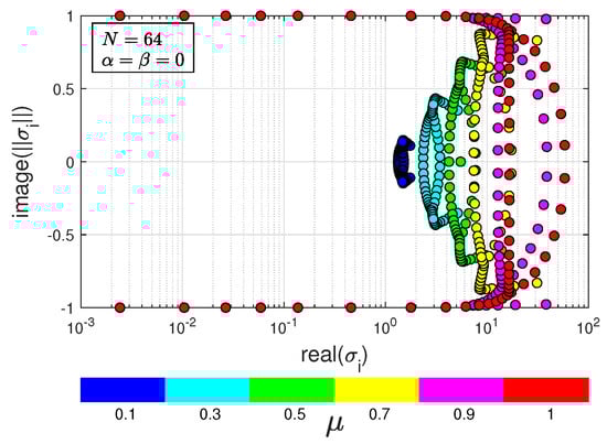
Figure 2. Eigenvalues of ${ }_C{\mathbf{D}}_l^{\mu }$: $N=64,\alpha =\beta =0$.

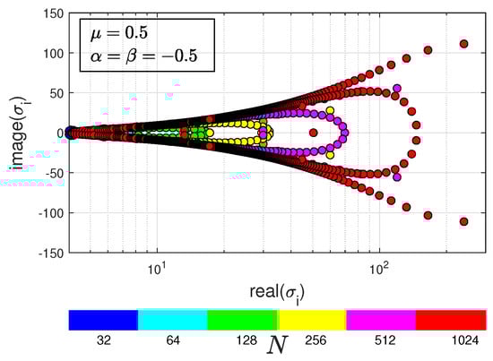
Figure 3. Eigenvalues of ${ }_C{\mathbf{D}}_l^{0.5}$: $\alpha =\beta =-0.5$.

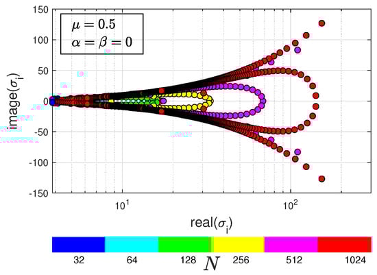
Figure 4. Eigenvalues of ${ }_C{\mathbf{D}}_l^{0.5}$: $\alpha =\beta =0$.

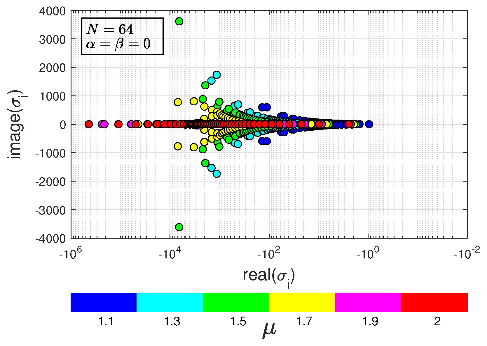
Figure 5 shows the distribution of the spectrum of ${ }_{RL}{\mathbf{D}}_l^{\mu }$ with different $\mu$ = 1.1:0.2:1.9 and 2 for Legendre–Gauss–Lobatto points of $N=64$. It is observed that the real parts of the eigenvalues are negative for all cases. Hence, we estimate that ${ }_{RL}{\mathbf{D}}_l^{\mu }$ is semi-negative definite for all $1<\mu \le 2$. For fixed $\mu =1.5$, Figure 6 demonstrates that, with increasing N, the eigenvalues are also more scattered away from the axis.

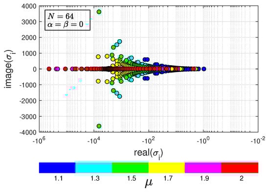
Figure 5. Eigenvalues of ${ }_{RL}{\mathbf{D}}_l^{\mu }$: $\alpha =\beta =0$.

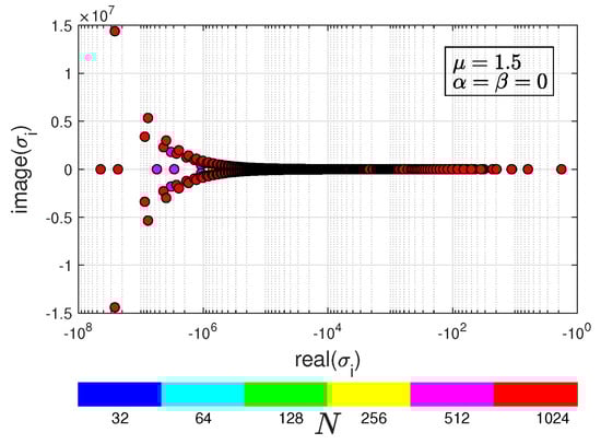
Figure 6. Eigenvalues of ${ }_{RL}{\mathbf{D}}_l^{1.5}$: $\alpha =\beta =0$.

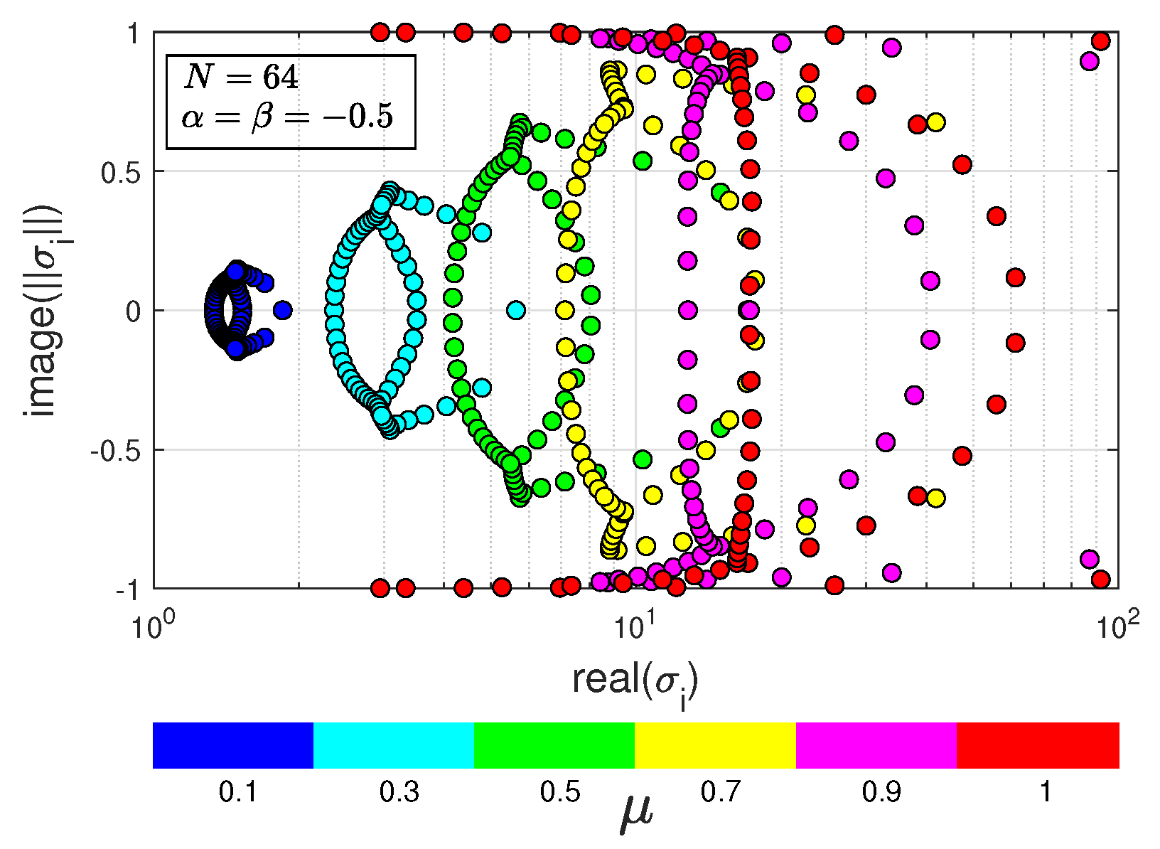
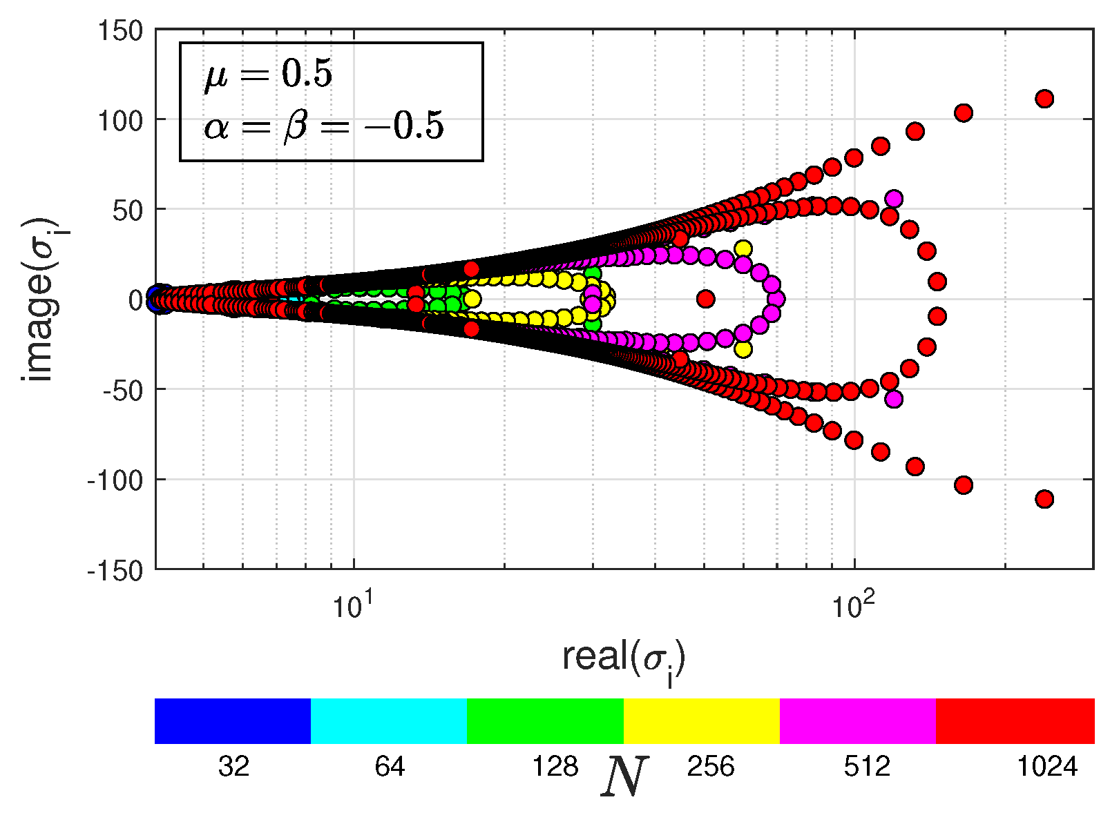
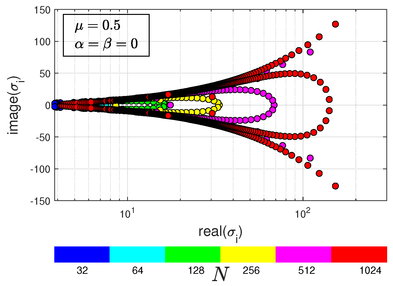
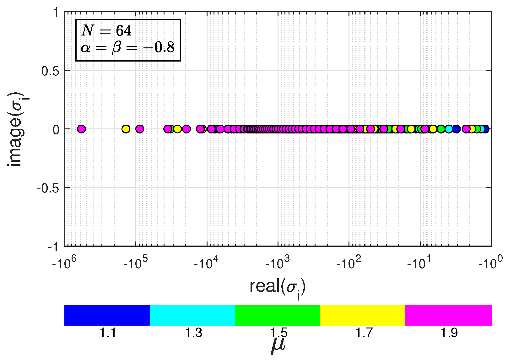
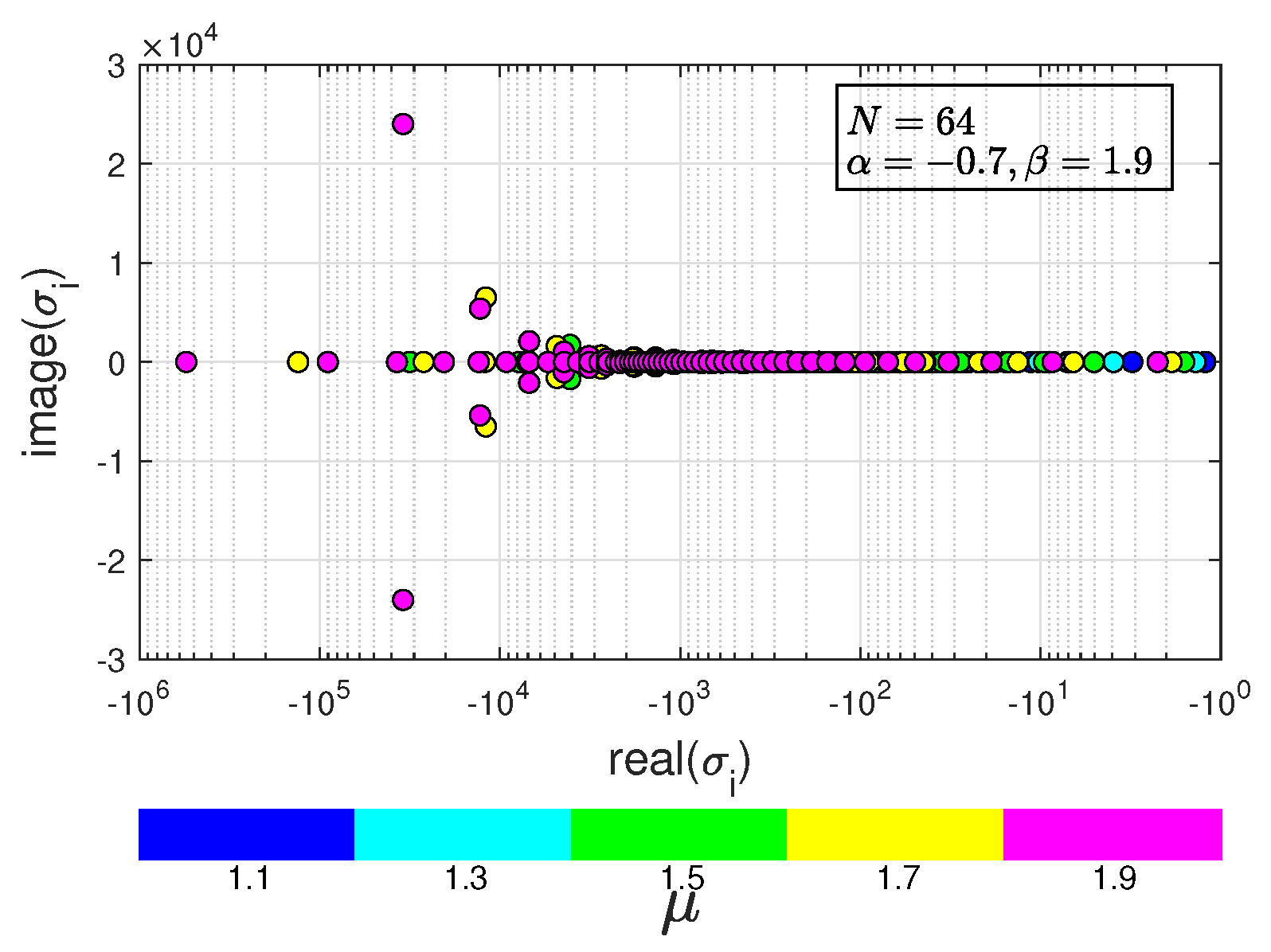
It is verified that the Riesz fractional derivative is self-adjoint and positive definite [36]. Figure 7 shows the distribution of the spectrum of ${ }_{RZ}{\mathbf{D}}^{\mu }$ with different $\mu$ = 1.1, 1.3, 1.5, 1.7, 1.9 for Jacobi–Gauss–Lobatto points of $\alpha =\beta =-0.8$, $N=64$. Figure 8 shows the distribution of the spectrum of ${ }_{RZ}{\mathbf{D}}^{\mu }$ for Jacobi–Gauss–Lobatto points of $\alpha =-0.7$, $\beta =1.9,N=64$. It is observed that the real parts of the eigenvalues are negative for all cases.

Figure 7. Eigenvalues of ${ }_{RZ}{\mathbf{D}}^{\mu }$: $\alpha =\beta =-0.8$.

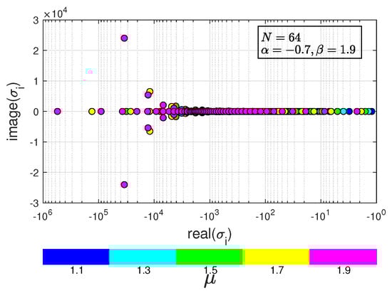
Figure 8. Eigenvalues of ${ }_{RZ}{\mathbf{D}}^{\mu }$: $\alpha =-0.7,\beta =1.9$.

5. Applications in Fractional Eigenvalue Problems

Eigenvalue problems are of importance in the theory and application of partial differential equations. Duan et al. [37] studied fractional eigenvalue problems. Reutskiy [38] presented a numerical method to solve fractional eigenvalue problems based on external excitation and the backward substitution method. He et al. [39] computed second-order fractional eigenvalue problems with the Jacobi–Davidson method. Gupta and Ranta [40] applied the Legendre wavelet method to solve fractional eigenvalue problems.

Example 1. 

Let $1<\mu <2$. Consider the boundary value problem

$$\left\{\begin{array}{c}{ }_C{\mathrm{D}}_{0,x}^{\mu }u\left(x\right)+\lambda u\left(x\right)=0,\hfill \\ pu\left(0\right)-r{u}^{\prime }\left(0\right)=0,qu\left(1\right)+s{u}^{\prime }\left(1\right)=0.\hfill \end{array}\right.$$

(33)

where $p,q,r,s\ge 0$ such that $p^2+r^2\ne 0$ and $q^2+s^2\ne 0$. Our test is for $p=q=1,r=s=0.$ This problem is also solved in [37,38,39,40]. For $\mu =1.8$, the first nine eigenvalues are listed in Table 1, together with the results given in [37,38,39,40] for comparison. Meanwhile, Table 2 lists the first six eigenvalues for $\mu =1.6$ which can be compared with the results in [37,38,40].

Table 1. The first nine eigenvalues of Example 1, computed with the Chebyshev collocation method ($\alpha =\beta =-0.5$) with $\mu =1.8$ and $N=200$.

$\mathit{\lambda }$	Our Method	[40]	[38]	[39]	[37]
${\lambda }_1$	9.45685689126	9.4568568891	9.4568568892	9.4997	9.4569
${\lambda }_2$	28.47687912479	28.4768791170	28.4768791186	28.5116	28.4769
${\lambda }_3$	62.20037779983	62.2003777331	62.2003777529	62.3239	62.2004
${\lambda }_4$	97.06323747284	97.0632373708	97.0632377552	97.0896	97.0632
${\lambda }_5$	155.45013805266	155.4501373840	155.4499080962	155.6972	-
${\lambda }_6$	196.59593024267	196.5959302453	196.5986985127	196.5152	-
${\lambda }_7$	301.52706976868	-	-	304.19 + 3.00i	-
${\lambda }_8$	306.72685026127	-	-	304.19 + 3.00i	-
${\lambda }_9$	461.179 + 43.050i	-	-	461.24 + 43.29i	-

Table 2. The first six eigenvalues of Example 1, computed with the Chebyshev collocation method ($\alpha =\beta =-0.5$) with $\mu =1.6$ and $N=200$.

$\mathit{\lambda }$	Our Method	[40]	[38]	[37]
${\lambda }_1$	13.420474051	13.42047399	13.4204739885	13.4205
${\lambda }_2$	14.645442473	14.64544252	14.6454425351	14.6454
${\lambda }_3$	47.292859 + 18.850956i	47.292858 + 18.850956i	-	-
${\lambda }_4$	91.705190 + 43.625498i	91.705189 + 43.625496i	-	-
${\lambda }_5$	145.569415 + 75.805031i	145.569416 + 75.805025i	-	-
${\lambda }_6$	207.859129 + 114.486222i	207.859147 + 114.486204i	-	-

When $\mu =2$, the analytic solution of the problem is ${\lambda }_n={\left(n\pi \right)}^2,n=1,2,\cdots$ (see [39]). The first six eigenvalues evaluated with the Chebyshev spectral collocation method (with $\alpha =\beta =-0.5$) and the errors between the numerical and analytic solutions are listed in the last two columns of Table 3. We also consider what happens when μ moves closer to 2. The first six eigenvalues for $\mu =1.9,1.999,1.9999,1.99999,1.999999$ are listed in Table 3 and Table 4. It is observed that the corresponding eigenvalues move increasingly closer to those of $\mu =2$.

Table 3. The first six eigenvalues of Example 1, computed with the Chebyshev collocation method ($\alpha =\beta =-0.5$) with $\mu =1.9999,1.99999,1.999999$ and $N=200$.

$\mathit{\lambda }$	$\mathit{\mu }=1.9999$	$\mathit{\mu }=1.99999$	$\mathit{\mu }=1.999999$	$\mathit{\mu }=2$	Error
${\lambda }_1$	9.8691292203	9.8695568729	9.8695996482	9.86960440108	1.073 $\times {10}^{-11}$
${\lambda }_2$	39.4719645919	39.4777722446	39.4783530678	39.47841760434	1.995 $\times {10}^{-11}$
${\lambda }_3$	88.8081881526	88.8246142309	88.8262570696	88.82643960980	7.148 $\times {10}^{-12}$
${\lambda }_4$	157.8754859530	157.9098514892	157.9132885198	157.91367041743	8.527 $\times {10}^{-14}$
${\lambda }_5$	246.6748284659	246.7335809315	246.7394571083	246.74011002723	1.336 $\times {10}^{-12}$
${\lambda }_6$	355.2042026720	355.2956013900	355.3047427196	355.30575843924	2.035 $\times {10}^{-11}$

Table 4. The first six eigenvalues of Example 1, computed with the Chebyshev collocation method ($\alpha =\beta =-0.5$) with different $\mu$ and $N=200$.

$\mathit{\lambda }$	$\mathit{\mu }=1.9$	$\mathit{\mu }=1.9$ [40]	$\mathit{\mu }=1.999$	$\mathit{\mu }=1.999$ [39]
${\lambda }_1$	9.5141431295	9.5141431288	9.8648626632	9.8648
${\lambda }_2$	33.5956714125	33.5956714089	39.4139459491	39.4139
${\lambda }_3$	73.0390172335	73.0390172163	88.6441581077	88.6442
${\lambda }_4$	124.4185311384	124.4185311250	157.5323069955	157.5325
${\lambda }_5$	191.1460514291	191.1460515330	246.0882332022	246.0886
${\lambda }_6$	267.9451997398	267.9452006460	354.2916713396	354.2922

For $\mu =1.1,1.3,1.5$, the first six eigenvalues are listed in Table 5, which are comparable with the results in [40]. It is shown that at least 5–6 digits after the decimal point are consistent. The eigenvalues for other cases of μ are also comparable with the results in [40], which are similar, so we do not list them here.

Table 5. The first six eigenvalues of Example 1, computed with the Chebyshev collocation method ($\alpha =\beta =-0.5$) with $\mu =1.1,1.3,1.5$ and $N=200$.

$\mathit{\lambda }$	$\mathit{\mu }=1.1$	$\mathit{\mu }=1.3$	$\mathit{\mu }=1.5$
${\lambda }_1$	1.3531852 + 7.2497408i	5.4727766 + 8.2732647i	11.1466676 + 6.1222836i
${\lambda }_2$	2.8098353 + 15.7308531i	13.3926574 + 21.8112244i	33.3136683 + 23.1298984i
${\lambda }_3$	4.3033960 + 24.6907235i	22.3712536 + 37.9533918i	61.1959645 + 46.6510167i
${\lambda }_4$	5.8291184 + 33.9686708i	32.1686781 + 55.9626406i	93.8181576 + 75.3667762i
${\lambda }_5$	7.3824934 + 43.4883769i	42.6472214 + 75.4712271i	130.5448587 + 108.4998614i
${\lambda }_6$	8.9599335 + 53.2043853i	53.7149929 + 96.2501648i	170.9467051 + 145.5427194i

From the results in Table 1, Table 2, Table 3, Table 4 and Table 5, it is shown that our method is reliable for the evaluation of the eigenvalues.

Example 2. 

Let $1<\mu <2$. Consider the eigenvalue problem of the Riesz derivative

$$\left\{\begin{array}{c}{ }_{RZ}{\mathrm{D}}_x^{\mu }u\left(x\right)+\lambda u\left(x\right)=0,\hfill \\ u(-1)=0,u\left(1\right)=0.\hfill \end{array}\right.$$

(34)

We solve the eigenvalue problem (34) using the Jacobi spectral collocation method. It is known that the Riesz fractional operator is self-adjoint and positive definite in a proper Sobolev space [36]. This fact is confirmed by numerical tests. It is observed that the discrete Riesz fractional differentiation matrix is strictly diagonally dominant with a negative diagonal for every value of parameter $1<\mu <2,\alpha ,\beta >-1,N$. The same problem has been studied using the Jacobi–Galerkin spectral method [36]. The first five eigenvalues obtained with the proposed method are listed in Table 6 and Table 7, together with the eigenvalues given in [36] for comparison.

Table 6. The first five eigenvalues of Example 2, computed with the Legendre collocation method ($\alpha =\beta =0$) with $\mu =1.2,1.4$ and $N=200$.

$\mathit{\lambda }$	$\mathit{\mu }=1.2$		$\mathit{\mu }=1.4$
	Our Method	[36]	Our Method	[36]
${\lambda }_1$	1.297024021884	1.296995777	1.483262055566	1.4832334320
${\lambda }_2$	3.486806460504	3.486730536	4.458260013435	4.4581739838
${\lambda }_3$	5.911808693986	5.911679975	8.150874006594	8.1507167266
${\lambda }_4$	8.534627231336	8.534441423	12.424593370123	12.424353637
${\lambda }_5$	11.292675855564	11.29243001	17.162678802344	17.162347657

Table 7. The first five eigenvalues of Example 2, computed with the Legendre collocation method ($\alpha =\beta =0$) with $\mu =1.6,1.8$ and $N=200$.

$\mathit{\lambda }$	$\mathit{\mu }=1.6$		$\mathit{\mu }=1.8$
	Our Method	[36]	Our Method	[36]
${\lambda }_1$	1.728321890005	1.72829595710	2.048752746738	2.04873498313
${\lambda }_2$	5.756434650807	5.75634828003	7.503181981160	7.50311692608
${\lambda }_3$	11.312063027525	11.3118933010	15.800031154322	15.7998941633
${\lambda }_4$	18.177615608424	18.1773428791	26.724474991011	26.7242432849
${\lambda }_5$	26.187596954514	26.1872040516	40.114581604547	40.1142338051

From the results in Table 6 and Table 7, we conclude that the presented method is reliable in solving eigenvalue problems.

6. Applications in Fractional Differential Equations

6.1. Fractional Initial Value Problems

The basic fractional initial value problem reads

$$\begin{array}{cc}\hfill & { }_C{\mathrm{D}}_{a,x}^{\mu }u\left(x\right)=f(u,x),m-1<\mu <m,\hfill \\ \hfill & u^{\left(k\right)}\left(a\right)=u_k,k=0,\cdots ,m-1.\hfill \end{array}$$

(35)

For the well posedness of (35), we refer to [11]. For $0<\mu \le 1,$ the discrete system of (35) reads

$${\mathbf{D}}^{\mu }\mathbf{u}=f(\mathbf{u},\mathbf{x})$$

with the collocation point vector $\mathbf{x}={[x_1,\cdots ,x_N]}^T$, the unknown $\mathbf{u}$ that approximates the exact solution at the collocation vector, and the differentiation matrix ${\mathbf{D}}^{\mu }$ with respect to the fractional derivative ${ }_C{\mathrm{D}}_{a,x}^{\mu }$. We obtain the numerical solution $u_N\left(\mathbf{x}\right)=\mathbf{u}\approx u\left(\mathbf{x}\right)$ by solving the system.

While exact solutions are known in the following examples, the error $E_{\infty }$ between the exact and numerical solutions is measured with

$$E_{\infty }:=\underset{1\le i\le N}{max}\{\parallel u\left(t_i\right)-u_N\left(t_i\right)\parallel \},$$

where $u_N\left(t\right)$ is the numerical solution and $t_i$ denotes the mapped collocation points (Jacobi–Gauss–Lobatto points). The numerical convergence order is estimated with

$$CO:=-\frac{log\left(E_{\infty }\left(N_1\right)\right)-log\left(E_{\infty }\left(N_2\right)\right)}{log\left(N_1\right)-log\left(N_2\right)}.$$

(36)

where $N_1$ and $N_2$ are two different degrees of freedom. We employ $CO$ to measure numerically the convergence order, e.g., the convergence rate likes $O\left(N^{-CO}\right)$.

Example 3. 

Let $0<\mu <1$. Consider the scalar linear fractional differential equation

$${ }_C{\mathrm{D}}_{0,t}^{\mu }u\left(t\right)=f\left(t\right),t\in (0,T],u\left(0\right)=u_0.$$

(37)

The right-hand-side term $f\left(t\right)$ is chosen so that the exact solution satisfies one of the following cases:

C11. 

$u\left(t\right)={\sum }_{k=1}^5\frac{t^{k\sigma }}{k},\sigma >0,t\in (0,2],u_0=0.$

C12. 

$u\left(t\right)=tsin\left(t\right),t\in (0,2\pi ],u_0=0.$

C13. 

$u\left(t\right)=E_{\mu ,1}(-t^{\mu }),t\in (0,3],u_0=1.$

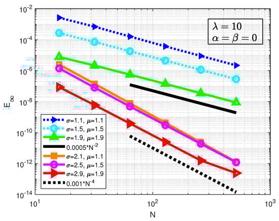
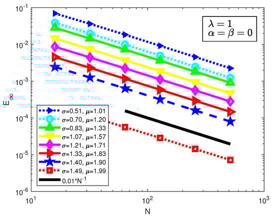
For case C11, the source function is exactly $f\left(t\right)={\sum }_{k=1}^5\frac{\mathsf{\Gamma }(k\sigma +1)t^{k\sigma -\mu }}{k\mathsf{\Gamma }(k\sigma -\mu +1)}$. Since the solution u has low regularity if $\sigma >0$ is a small non-integer, the convergence order is limited. The errors $E_{\infty }$ and convergence orders $CO$ are listed in Table 8 and Table 9. It is shown that the convergence order for this case is clearly $O\left(N^{-2\sigma }\right)$ if $\sigma >0$ is a small non-integer. When σ is an integer, the solution u is smooth and exactly belongs to ${\mathbb{P}}_{5\sigma }$. Hence, we only need $N=5\sigma$ to resolve this problem. Table 10 lists the errors $E_{\infty }$ which show that machine precision is almost achieved for the case when $N=5\sigma$.

Table 8. The error $E_{\infty }$ and convergence order $CO$ of C11 in Example 3, computed with the Chebyshev collocation method ($\alpha =\beta =-0.5$) for $\sigma =2.5$.

N	$\mathit{\mu }=0.2$		$\mathit{\mu }=0.4$		$\mathit{\mu }=0.6$		$\mathit{\mu }=0.8$
	E∞	CO	E∞	CO	E∞	CO	E∞	CO
12	6.434$\times {10}^{-6}$	-	1.329$\times {10}^{-5}$	-	2.627$\times {10}^{-5}$	-	5.384$\times {10}^{-5}$	-
20	2.356$\times {10}^{-7}$	6.47	5.692$\times {10}^{-7}$	6.17	1.109$\times {10}^{-6}$	6.20	1.968$\times {10}^{-6}$	6.48
28	4.373$\times {10}^{-8}$	5.01	1.055$\times {10}^{-7}$	5.01	2.055$\times {10}^{-7}$	5.01	3.648$\times {10}^{-7}$	5.01
36	1.244$\times {10}^{-8}$	5.00	2.998$\times {10}^{-8}$	5.01	5.840$\times {10}^{-8}$	5.01	1.037$\times {10}^{-7}$	5.01
44	4.559$\times {10}^{-9}$	5.00	1.099$\times {10}^{-8}$	5.00	2.140$\times {10}^{-8}$	5.00	3.800$\times {10}^{-8}$	5.00
52	1.977$\times {10}^{-9}$	5.00	4.764$\times {10}^{-9}$	5.00	9.280$\times {10}^{-9}$	5.00	1.648$\times {10}^{-8}$	5.00
60	9.664$\times {10}^{-10}$	5.00	2.328$\times {10}^{-9}$	5.00	4.536$\times {10}^{-9}$	5.00	8.054$\times {10}^{-9}$	5.00
68	5.168$\times {10}^{-10}$	5.00	1.245$\times {10}^{-9}$	5.00	2.426$\times {10}^{-9}$	5.00	4.307$\times {10}^{-9}$	5.00

Table 9. The error $E_{\infty }$ and convergence order $CO$ of C11 in Example 3, computed with the Chebyshev collocation method ($\alpha =\beta =-0.5$) for $\mu =0.5$.

N	$\mathit{\sigma }=0.5$		$\mathit{\sigma }=1.2$		$\mathit{\sigma }=1.8$		$\mathit{\sigma }=2.2$
	E∞	CO	E∞	CO	E∞	CO	E∞	CO
8	4.044$\times {10}^{-2}$	-	1.236$\times {10}^{-3}$	-	1.263$\times {10}^{-3}$	-	7.994$\times {10}^{-2}$	-
16	2.036$\times {10}^{-2}$	0.99	2.410$\times {10}^{-4}$	2.36	1.811$\times {10}^{-5}$	6.12	4.055$\times {10}^{-6}$	14.27
24	1.359$\times {10}^{-2}$	1.00	9.146$\times {10}^{-5}$	2.39	4.193$\times {10}^{-6}$	3.61	6.775$\times {10}^{-7}$	4.41
32	1.020$\times {10}^{-2}$	1.00	4.591$\times {10}^{-5}$	2.40	1.487$\times {10}^{-6}$	3.60	1.908$\times {10}^{-7}$	4.41
40	8.158$\times {10}^{-3}$	1.00	2.689$\times {10}^{-5}$	2.40	6.658$\times {10}^{-7}$	3.60	7.143$\times {10}^{-8}$	4.40
48	6.799$\times {10}^{-3}$	1.00	1.737$\times {10}^{-5}$	2.40	3.453$\times {10}^{-7}$	3.60	3.201$\times {10}^{-8}$	4.40
56	5.828$\times {10}^{-3}$	1.00	1.200$\times {10}^{-5}$	2.40	1.982$\times {10}^{-7}$	3.60	1.624$\times {10}^{-8}$	4.40
64	5.100$\times {10}^{-3}$	1.00	8.708$\times {10}^{-6}$	2.40	1.226$\times {10}^{-7}$	3.60	9.024$\times {10}^{-9}$	4.40

Table 10. The error $E_{\infty }$ of C11 in Example 3, computed with the Chebyshev collocation method ($\alpha =\beta =-0.5$).

$\mathit{N}\left(\mathit{\sigma }\right)$	$\mathit{\mu }=0.1$	$\mathit{\mu }=0.3$	$\mathit{\mu }=0.5$	$\mathit{\mu }=0.7$	$\mathit{\mu }=0.9$	$\mathit{\mu }=0.99$
5(1)	1.776$\times {10}^{-14}$	1.599$\times {10}^{-14}$	1.954$\times {10}^{-14}$	1.776$\times {10}^{-14}$	2.309$\times {10}^{-14}$	1.599$\times {10}^{-14}$
10(2)	2.387$\times {10}^{-12}$	2.132$\times {10}^{-12}$	2.103$\times {10}^{-12}$	2.558$\times {10}^{-12}$	2.217$\times {10}^{-12}$	2.103$\times {10}^{-12}$
15(3)	5.912$\times {10}^{-11}$	2.728$\times {10}^{-11}$	2.819$\times {10}^{-11}$	6.003$\times {10}^{-11}$	2.728$\times {10}^{-11}$	3.547$\times {10}^{-11}$

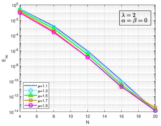
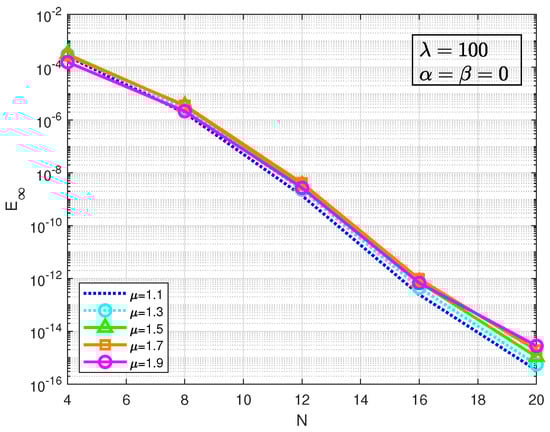
For case C12, the solution is smooth. Thus, we expect the convergence order to be exponential. The errors $E_{\infty }$ in Table 11 show “spectral accuracy".

Table 11. The error $E_{\infty }$ of C12 in Example 3, computed with the Chebyshev collocation method ($\alpha =\beta =-0.5$).

N	$\mathit{\mu }=0.1$	$\mathit{\mu }=0.3$	$\mathit{\mu }=0.5$	$\mathit{\mu }=0.7$	$\mathit{\mu }=0.9$	$\mathit{\mu }=0.99$
6	9.557$\times {10}^{-3}$	2.978$\times {10}^{-2}$	5.208$\times {10}^{-2}$	8.299$\times {10}^{-2}$	1.377$\times {10}^{-1}$	1.931$\times {10}^{-1}$
10	7.758$\times {10}^{-6}$	2.475$\times {10}^{-5}$	4.212$\times {10}^{-5}$	6.440$\times {10}^{-5}$	1.072$\times {10}^{-4}$	1.626$\times {10}^{-4}$
14	1.522$\times {10}^{-9}$	4.709$\times {10}^{-9}$	8.159$\times {10}^{-9}$	1.212$\times {10}^{-8}$	2.043$\times {10}^{-8}$	3.113$\times {10}^{-8}$
18	2.749$\times {10}^{-13}$	5.519$\times {10}^{-13}$	5.405$\times {10}^{-13}$	1.002$\times {10}^{-12}$	1.333$\times {10}^{-12}$	2.055$\times {10}^{-12}$
22	2.398$\times {10}^{-13}$	5.959$\times {10}^{-13}$	3.545$\times {10}^{-14}$	1.024$\times {10}^{-12}$	1.420$\times {10}^{-13}$	1.631$\times {10}^{-13}$

For case C13, the solution u has low regularity since the term $t^{\mu }$ is involved. Thus, the convergence order should be low. Table 12 and Table 13 list the errors $E_{\infty }$ and convergence orders $CO$, which show clearly that the convergence order is $O\left(N^{-2\mu }\right)$.

Table 12. The error $E_{\infty }$ and convergence order $CO$ of C13 in Example 3, computed with the Chebyshev collocation method ($\alpha =\beta =-0.5$).

N	$\mathit{\mu }=0.2$		$\mathit{\mu }=0.3$		$\mathit{\mu }=0.5$		$\mathit{\mu }=0.6$
	E∞	CO	E∞	CO	E∞	CO	E∞	CO
4	6.129$\times {10}^{-2}$	-	8.253$\times {10}^{-2}$	-	1.039$\times {10}^{-1}$	-	1.028$\times {10}^{-1}$	-
8	5.106$\times {10}^{-2}$	0.26	6.075$\times {10}^{-2}$	0.44	5.514$\times {10}^{-2}$	0.91	4.442$\times {10}^{-2}$	1.21
16	4.185$\times {10}^{-2}$	0.29	4.324$\times {10}^{-2}$	0.49	2.803$\times {10}^{-2}$	0.98	1.894$\times {10}^{-2}$	1.23
32	3.379$\times {10}^{-2}$	0.31	3.002$\times {10}^{-2}$	0.53	1.408$\times {10}^{-2}$	0.99	8.145$\times {10}^{-3}$	1.22
64	2.693$\times {10}^{-2}$	0.33	2.049$\times {10}^{-2}$	0.55	7.047$\times {10}^{-3}$	1.00	3.525$\times {10}^{-3}$	1.21
128	2.123$\times {10}^{-2}$	0.34	1.383$\times {10}^{-2}$	0.57	3.524$\times {10}^{-3}$	1.00	1.530$\times {10}^{-3}$	1.20
256	1.659$\times {10}^{-2}$	0.36	9.261$\times {10}^{-3}$	0.58	1.762$\times {10}^{-3}$	1.00	6.653$\times {10}^{-4}$	1.20
512	1.288$\times {10}^{-2}$	0.37	6.170$\times {10}^{-3}$	0.59	8.812$\times {10}^{-4}$	1.00	2.895$\times {10}^{-4}$	1.20

Table 13. The error $E_{\infty }$ and convergence order $CO$ of C13 in Example 3, computed with the Chebyshev collocation method ($\alpha =\beta =-0.5$).

N	$\mathit{\mu }=0.7$		$\mathit{\mu }=0.8$		$\mathit{\mu }=0.9$		$\mathit{\mu }=0.99$
	E∞	CO	E∞	CO	E∞	CO	E∞	CO
4	9.283$\times {10}^{-2}$	-	7.376$\times {10}^{-2}$	-	4.563$\times {10}^{-2}$	-	1.312$\times {10}^{-2}$	-
8	3.180$\times {10}^{-2}$	1.55	1.939$\times {10}^{-2}$	1.93	8.566$\times {10}^{-3}$	2.41	7.498$\times {10}^{-4}$	4.13
16	1.144$\times {10}^{-2}$	1.47	5.948$\times {10}^{-3}$	1.70	2.268$\times {10}^{-3}$	1.92	1.754$\times {10}^{-4}$	2.10
32	4.247$\times {10}^{-3}$	1.43	1.918$\times {10}^{-3}$	1.63	6.379$\times {10}^{-4}$	1.83	4.370$\times {10}^{-5}$	2.01
64	1.597$\times {10}^{-3}$	1.41	6.280$\times {10}^{-4}$	1.61	1.821$\times {10}^{-4}$	1.81	1.103$\times {10}^{-5}$	1.99
128	6.032$\times {10}^{-4}$	1.40	2.066$\times {10}^{-4}$	1.60	5.221$\times {10}^{-5}$	1.80	2.793$\times {10}^{-6}$	1.98
256	2.283$\times {10}^{-4}$	1.40	6.811$\times {10}^{-5}$	1.60	1.499$\times {10}^{-5}$	1.80	7.077$\times {10}^{-7}$	1.98
512	8.647$\times {10}^{-5}$	1.40	2.246$\times {10}^{-5}$	1.60	4.303$\times {10}^{-6}$	1.80	1.794$\times {10}^{-7}$	1.98

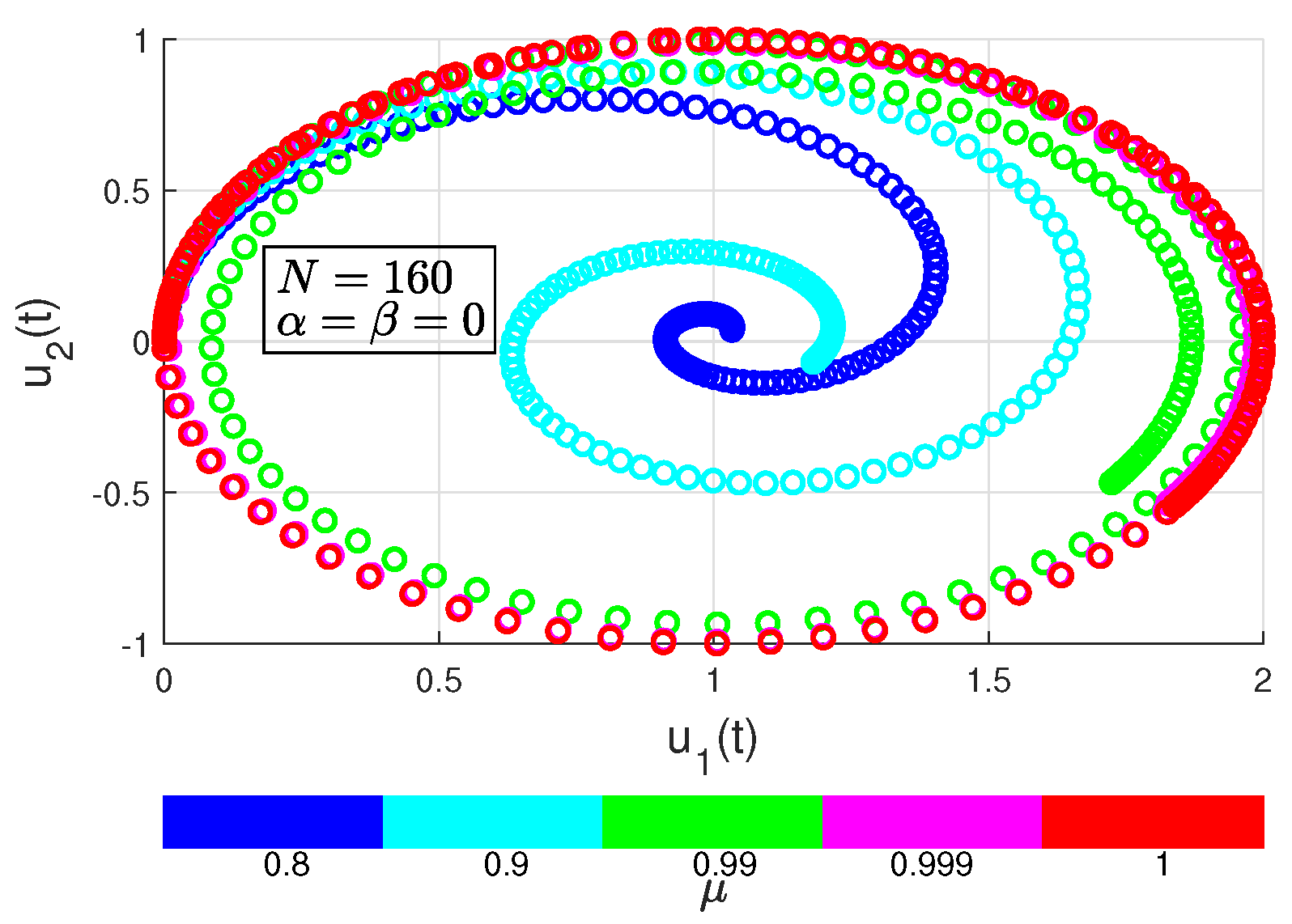
Example 4. 

Let $0<\mu <1$. Consider the linear fractional differential system

$$\left\{\begin{array}{c}{ }_C{\mathrm{D}}_{0,t}^{\mu }{u}_1\left(t\right)=u_2\left(t\right),\hfill \\ { }_C{\mathrm{D}}_{0,t}^{\mu }{u}_2\left(t\right)=-u_1\left(t\right)+1,0<t\le 10\hfill \end{array}\right.$$

(38)

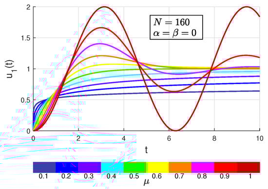
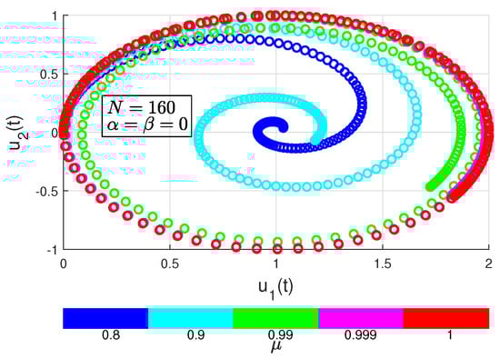
with the initial value $u_1\left(0\right)=u_2\left(0\right)=0$. If $\mu =1$, the solution of (38) is $u_1\left(t\right)=1-cos\left(t\right),u_2\left(t\right)=sin\left(t\right)$. We apply the Legendre spectral collocation method with $N=160$ to produce maximum errors of $E_{1,\infty }=2.3412e-12$ and $E_{2,\infty }=2.2929e-12$. We plot the curves of the numerical solution $u_1\left(t\right)$ for different μ in Figure 9. We plot the portrait of the phase plane $u_1\left(t\right)$ and $u_2\left(t\right)$ in Figure 10. The results show good agreement with the figures in [17].

Figure 9. Curves of numerical solution of Example 4.

Figure 10. Portrait of phase plane $u_1\left(t\right)$ and $u_2\left(t\right)$ of Example 4.

6.2. Fractional Boundary Value Problems

Let $1<\mu <2$. As a benchmark fractional boundary value problem, we consider the one-dimensional fractional Helmholtz equation as

$${\lambda }^{2}u\left(x\right)-{\mathrm{D}}_x^{\mu }u\left(x\right)=f\left(x\right),x\in (a,b),u\left(a\right)=u\left(b\right)=0,$$

(39)

where the fractional derivative operator ${\mathrm{D}}_x^{\mu }$ will be specified in the following examples. The discrete system of (39) in the spectral collocation method reads

$$\left({\lambda }^2\mathbf{I}-{\mathbf{D}}^{\mu }\right)\mathbf{u}=f\left(\mathbf{x}\right)$$

with the $(N-1)\times (N-1)$ identical matrix $\mathbf{I}$, the fractional differentiation matrix ${\mathbf{D}}^{\mu }$ (whose first and last row and column are removed) corresponding to the fractional derivative operator, the undetermined unknowns $\mathbf{u}=u_N\left(\mathbf{x}\right)$ and the interior collocation points $\mathbf{x}={[x_1,\cdots ,x_{N-1}]}^T$ (mapped into $(a,b)$).

Example 5. 

Consider Equation (39) with the Caputo derivative: ${\mathrm{D}}_x^{\mu }={ }_C{\mathrm{D}}_{a,x}^{\mu }$. The source term $f\left(x\right)$ is chosen so that the exact solution satisfies one of the following cases:

C21. 

$u\left(x\right)=x^{\sigma }-x^{2\sigma },\sigma >0,a=0,b=1.$

C22. 

$u\left(x\right)=sin\left(\pi x\right),a=-1,b=1.$

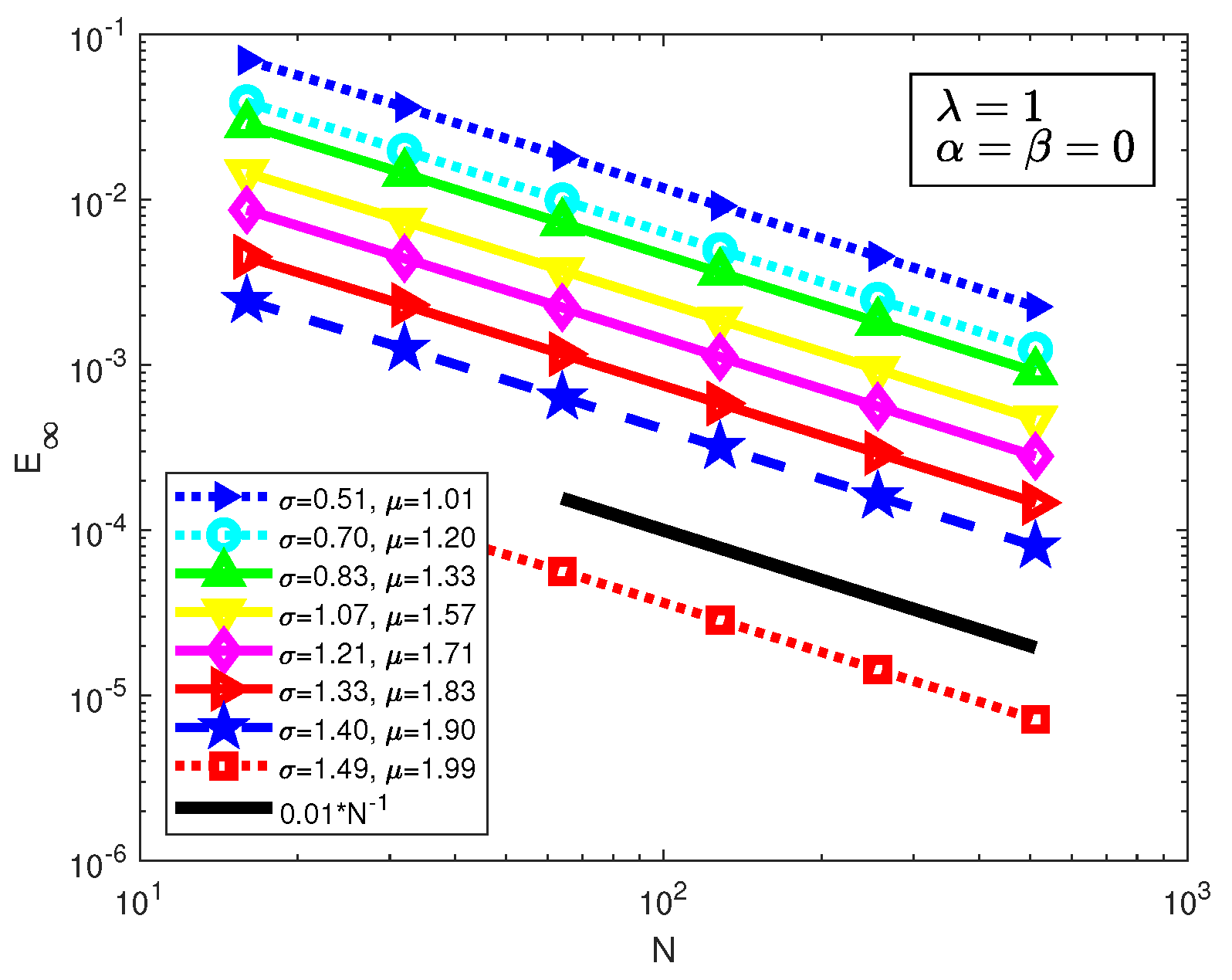
For case C21, since the solution u has low regularity if $\sigma >0$ is a small non-integer, the convergence order is limited. The errors $E_{\infty }$ are plotted in Figure 11 and Figure 12 for different $N,\sigma$ and μ. Figure 12 shows that the convergence order is of the first order. It is shown that the convergence order for this case depends on σ and μ. A possible estimate of the convergence order is $O\left(N^{-2(\sigma -\mu +1)}\right)$ if $\sigma >0$ is a small non-integer.

Figure 11. Errors of C21 of Example 5.

Figure 12. Errors of C21 of Example 5.

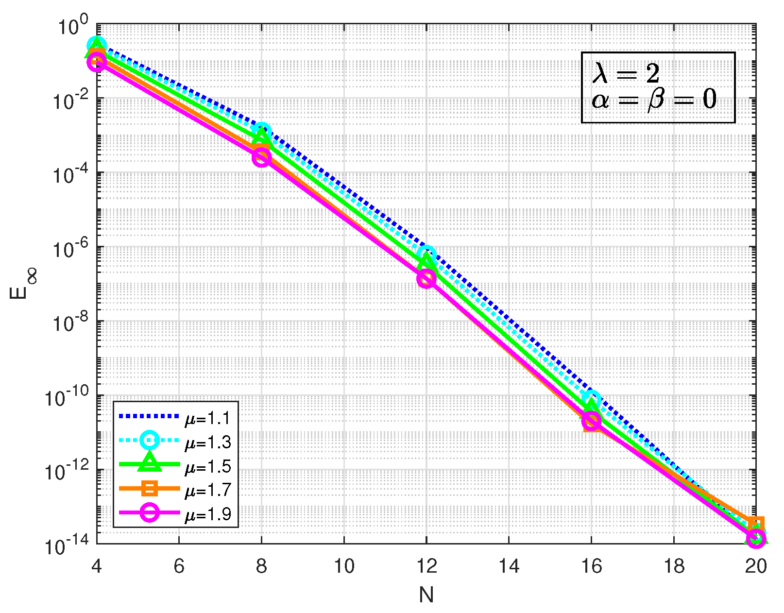
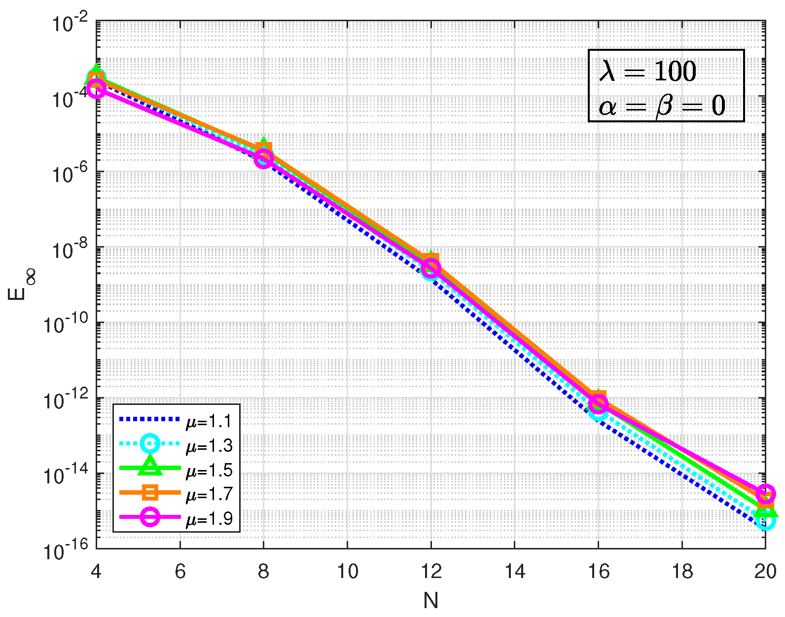
For case C22, the source function is approximated by

$$f\left(x\right)\approx \sum _{k=1}^L\frac{{(-1)}^k{\pi }^{2k+1}}{\mathsf{\Gamma }(2k+2-\mu )}{(x+1)}^{2k+1-\mu }$$

with a sufficiently large integer L (here, $L=50$). Since the solution is smooth, we expect the convergence order to be exponential. Figure 13 and Figure 14 plot the errors $E_{\infty }$, which show “spectral accuracy".

Figure 13. Errors of C22 of Example 5.

Figure 14. Errors of C22 of Example 5.

Example 6. 

Consider Equation (39) with the Riesz derivative ${\mathrm{D}}_x^{\mu }={ }_{RZ}{\mathrm{D}}_x^{\mu }$. The numerical test is performed for the fractional Poisson equation in two cases:

C31. 

$f\left(x\right)=1,\lambda =0,a=-1,b=1.$

C32. 

$f\left(x\right)=sin\left(\pi x\right),\lambda =0,a=-1,b=1.$

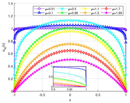
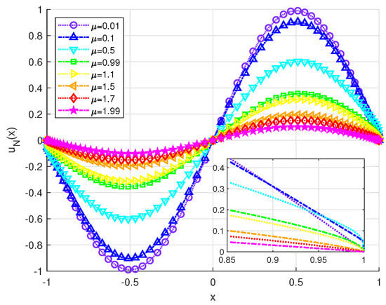
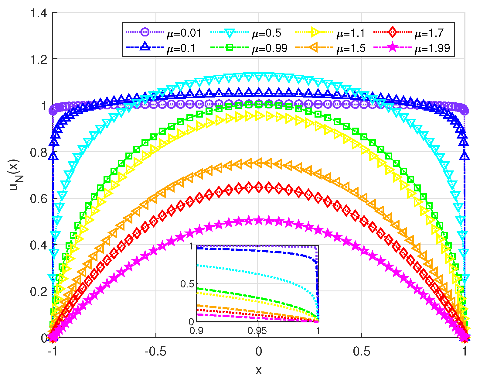
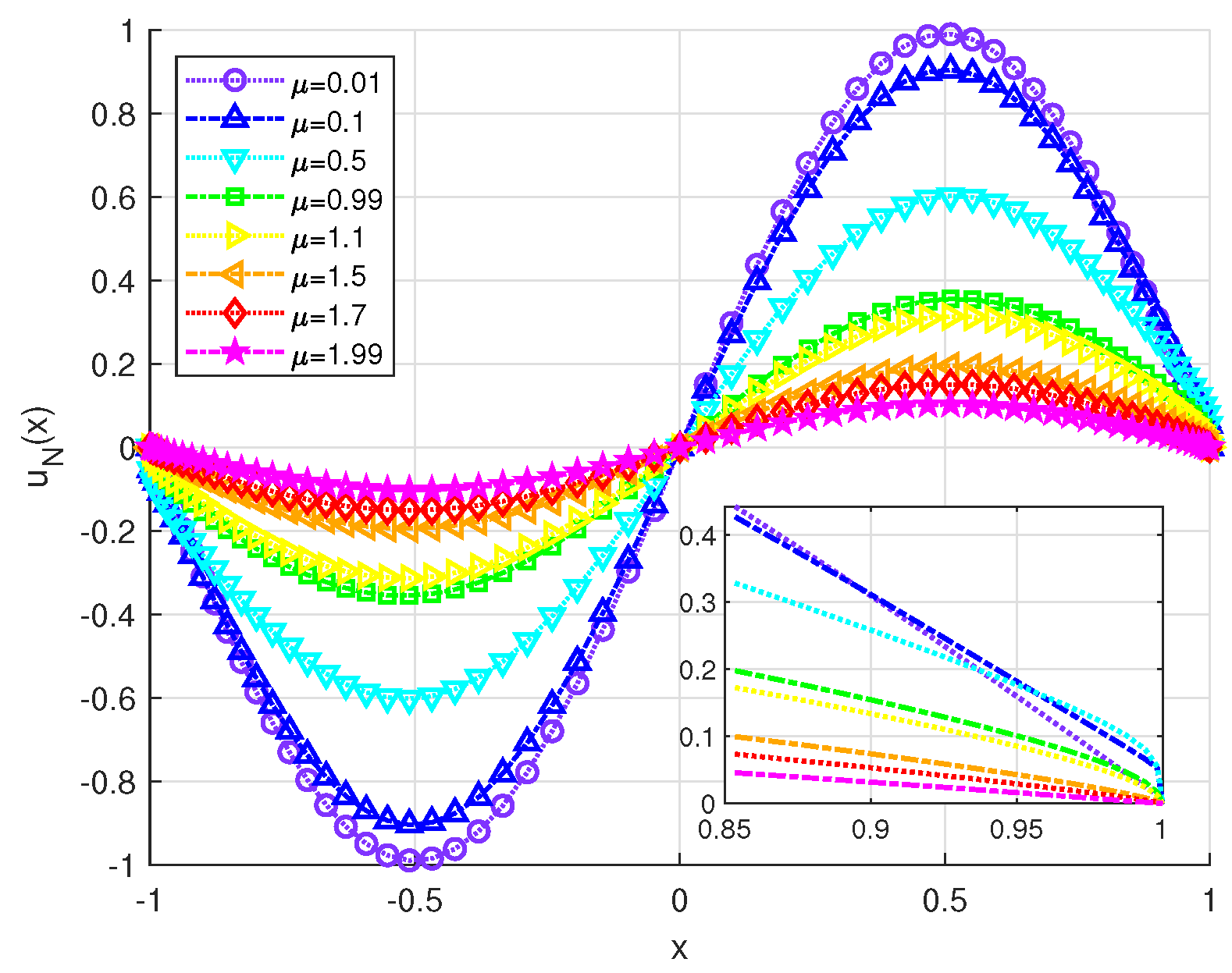
We solve the fractional Poisson problems with the Riesz derivative by employing the Legendre spectral collocation method ($\alpha =\beta =0$) with $N=64$. The profiles of the numerical solutions are plotted in Figure 15 and Figure 16. From a comparison with the curves in [41] (Figure 1 and Figure 4 (left)), the two groups of curves match very well.

Figure 15. Numerical solution of C31 of Example 6 with $N=64,\alpha =\beta =0$.

Figure 16. Numerical solution of C32 of Example 6 with $N=64,\alpha =\beta =0$.

6.3. Fractional Initial Boundary Value Problems

The fractional Burgers equation is a generalized model that describes weak nonlinearity propagation, such as in the acoustic phenomenon of a sound wave through a gas-filled tube. There are many publications that present analytical and numerical solutions to the Riemann–Liouville and Caputo fractional Burgers equations (see [27,42]). One of the fractional Burgers equations (FBEs) in one-dimensional form reads

$${\partial }_{t}u+u{\partial }_{x}u=ϵ{\mathrm{D}}_x^{\mu }u,(x,t)\in (a,b)\times (0,T]$$

(40)

with the boundary condition $u(a,t)=u(b,t)=0$ and the initial profile $u(x,0)=u_0\left(x\right)$. For the time discretization, we employ a semi-implicit time discretization scheme with step size $\tau$, namely the two-step Crank–Nicolson/leapfrog scheme. Then, the full discretization scheme reads:

$$\left\{\begin{array}{cc}\left(\mathbf{I}-ϵ\tau {\mathbf{D}}^{\mu }\right){\mathbf{u}}^{n+1}=\left(\mathbf{I}+ϵ\tau {\mathbf{D}}^{\mu }\right){\mathbf{u}}^{n-1}-2\tau \left(\mathrm{diag}\left({\mathbf{u}}^n\right)\mathbf{D}\right){\mathbf{u}}^n,\hfill & n\ge 1,\hfill \\ {\mathbf{u}}^1=\left(\mathbf{I}+ϵ\tau {\mathbf{D}}^{\mu }\right){\mathbf{u}}^0-\tau \left(\mathrm{diag}\left({\mathbf{u}}^0\right)\mathbf{D}\right){\mathbf{u}}^0\hfill \\ {\mathbf{u}}^0=u_0\left(\mathbf{x}\right),\hfill \end{array}\right.$$

(41)

where $\mathbf{D}$ is the first-order differentiation matrix. In the following examples, we always take $\alpha =\beta =0,N=360$ and $\tau ={10}^{-3}.$

Example 7. 

Consider Equation (40) with the Caputo derivative: ${\mathrm{D}}_x^{\mu }={ }_C{\mathrm{D}}_x^{\mu }$. The numerical test is performed for two cases of initial profiles:

C41. 

$u_0\left(x\right)=sin\left(\pi x\right),a=-1,b=1.$

C42. 

$u_0\left(x\right)=exp(-2x^2),a=-7,b=7.$

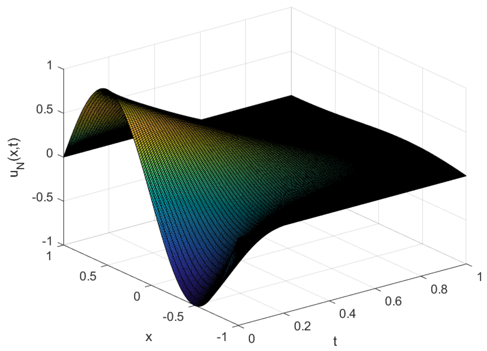
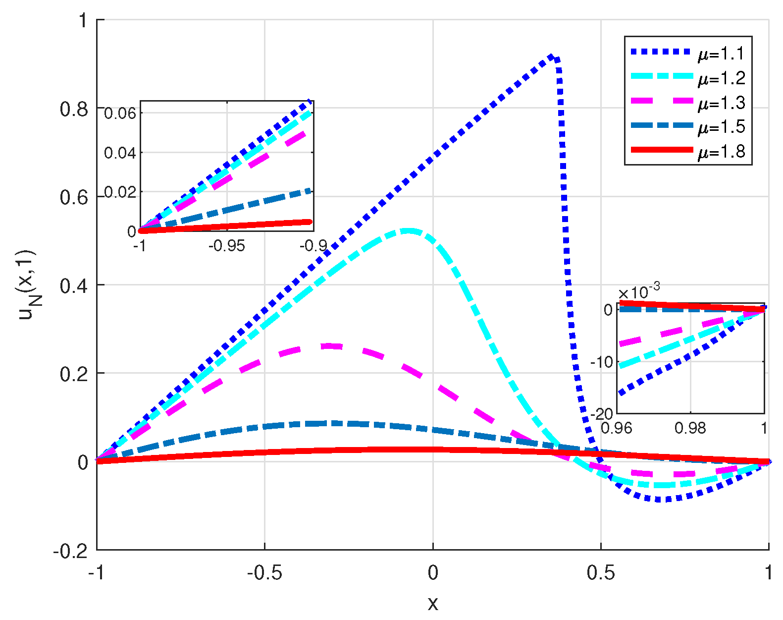
We first consider the initial profile with two peaks, i.e., case C41. The surface of the numerical solution is plotted in Figure 17 for $\mu =1.5$ and $T=1$. The evolution of the numerical solution is observed. The numerical solutions of the FBE at time $t=1$ are plotted in Figure 18 for different values of fractional order $\mu =1.1,1.2,1.3,1.5,1.8$.

Figure 17. Numerical solution of C41 of Example 7 with $u_0\left(x\right)=sin\left(\pi x\right)$.

Figure 18. Numerical solution of C41 of Example 7 with $u_0\left(x\right)=sin\left(\pi x\right)$.

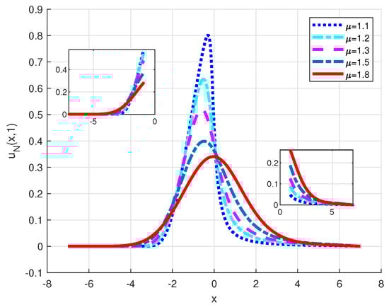
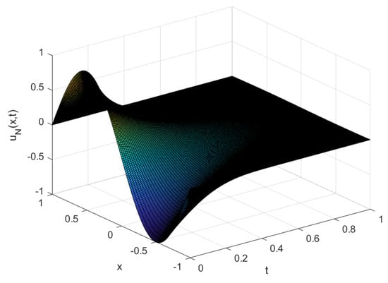
For case C42, the surface of the numerical solution for $\mu =1.5,T=1$ is plotted in Figure 19. The evolution of the numerical solution is observed. The numerical solutions of the FBE at time $t=1$ are plotted in Figure 20 for different values of fractional order $\mu =1.1,1.2,1.3,1.5,1.8$.

Figure 19. Numerical solution of C42 of Example 7 with $u_0\left(x\right)=exp(-x^2)$.

Figure 20. Numerical solution of C42 of Example 7 with $u_0\left(x\right)=exp(-x^2)$.

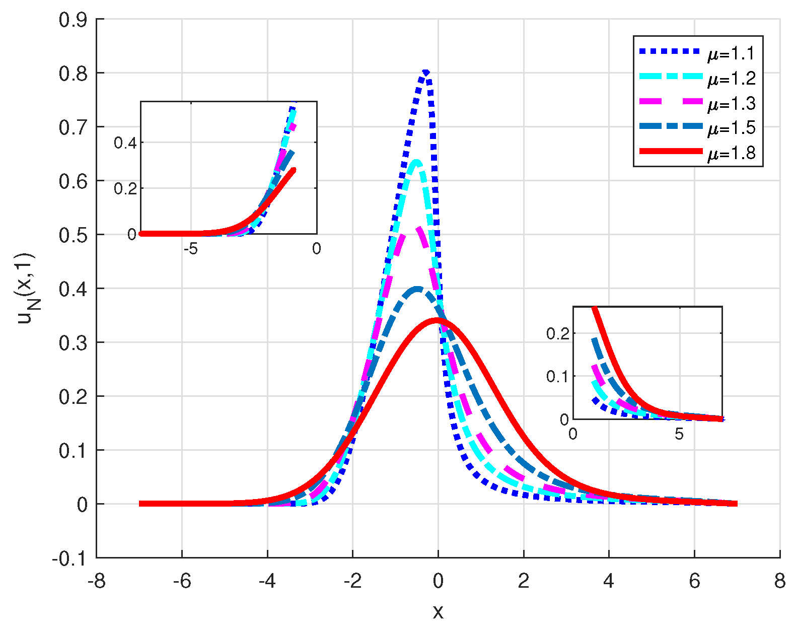
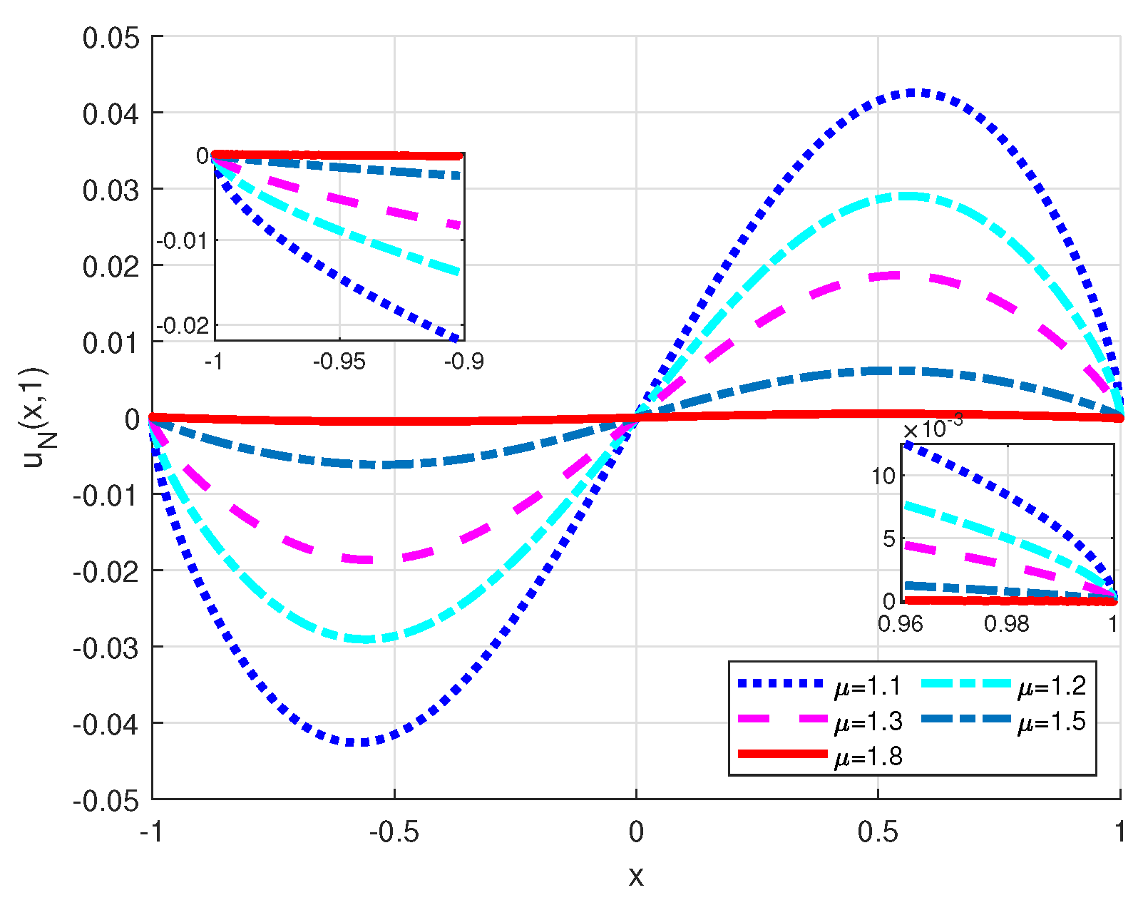
Example 8. 

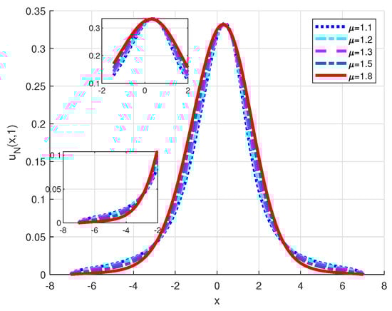
Consider Equation (40) with the Riesz derivative: ${\mathrm{D}}_x^{\mu }={ }_{RZ}{\mathrm{D}}_x^{\mu }$. The numerical test is performed for the same two initial profiles as in (7).

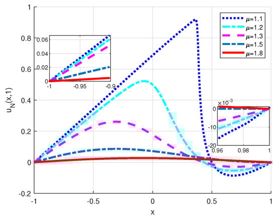
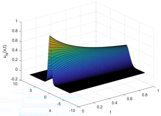
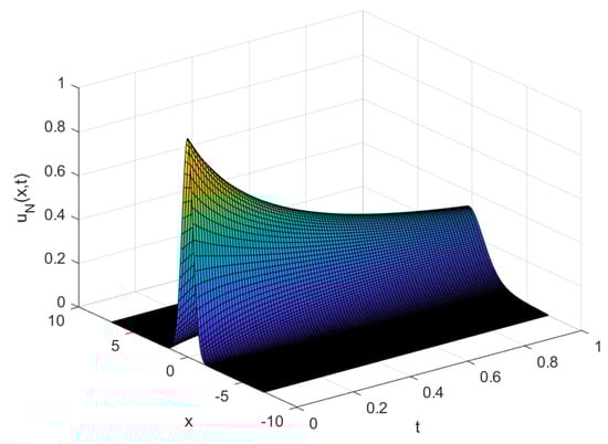
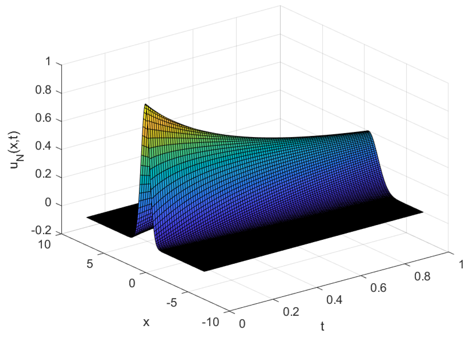
We proceed in the same way as in the above example. We first consider the initial profile with two peaks, i.e., case C41. The surface of the numerical solution is plotted in Figure 21 for $\mu =1.5,T=1$. The evolution of the numerical solution is observed. The numerical solutions of the FBE at time $t=1$ are plotted in Figure 22 for different values of fractional order $\mu =1.1,1.2,1.3,1.5,1.8$.

Figure 21. Numerical solution of Example 8 with $u_0\left(x\right)=sin\left(\pi x\right)$.

Figure 22. Numerical solution of Example 8 with $u_0\left(x\right)=sin\left(\pi x\right)$.

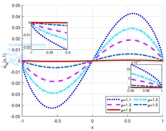
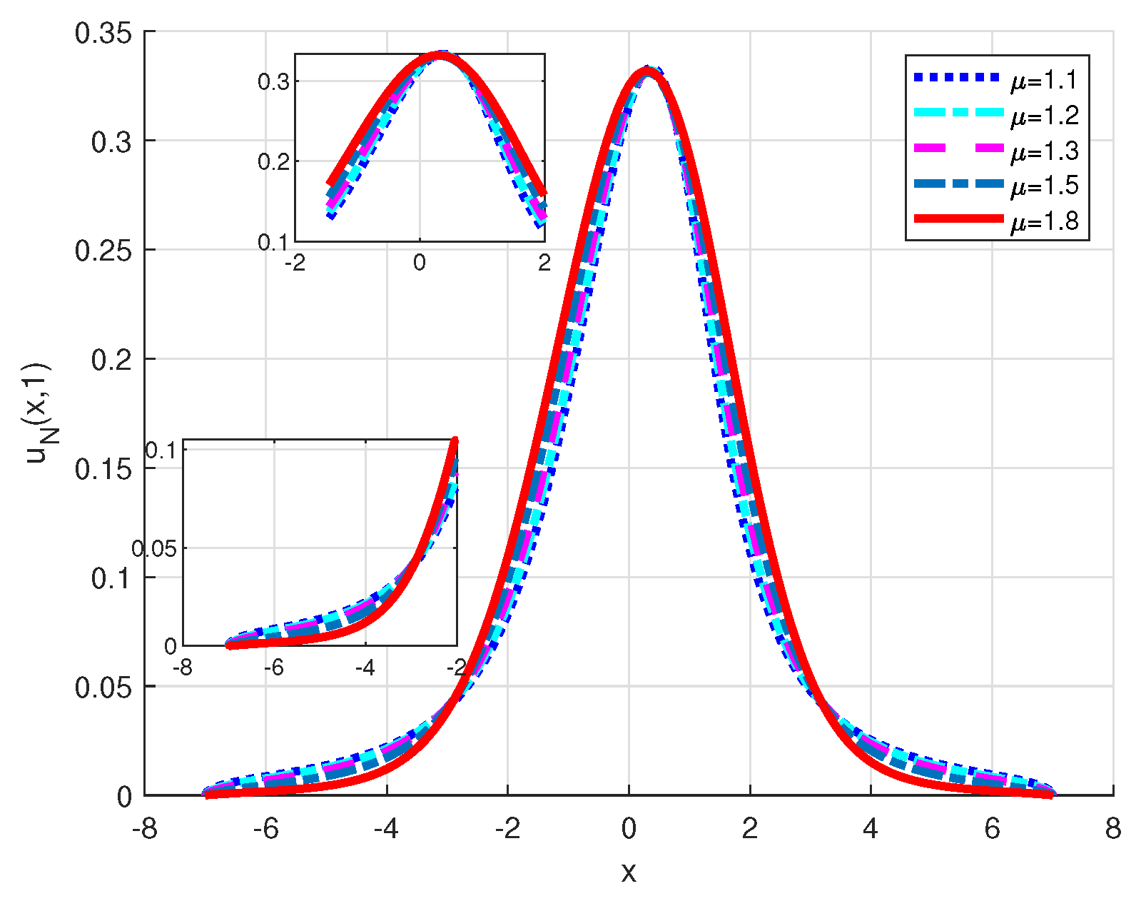
For case C42, the surface of the numerical solution is plotted in Figure 23 for $\mu =1.5,T=1$. The evolution of the numerical solution is observed. The numerical solutions of the FBE at time $t=1$ are plotted in Figure 24 for different values of fractional order $\mu =1.1,1.2,1.3,1.5,1.8$.

Figure 23. Numerical solution of Example 8 with $u_0\left(x\right)=exp(-x^2)$.

Figure 24. Numerical solution of Example 8 with $u_0\left(x\right)=exp(-x^2)$.

7. Conclusions

A fractional differentiation matrix is constructed by employing the Jacobi–Jacobi transformation between two indexes $({\alpha }_1,{\beta }_1)$ and $({\alpha }_2,{\beta }_2)$. In effect, the fractional differentiation matrix is given as a product of some special matrices. With the aid of this representation, the fractional differentiation matrix can be evaluated in a stable, fast, and efficient manner. This representation gives a direct way to form differentiation matrices with relatively fewer operations, which is easy to program. Another benefit of this representation is that the inverses of the differentiation matrices can be obtained in the meantime, which makes the discrete system easy to solve. We develop applications of the fractional differentiation matrix with the Jacobi spectral collocation method to fractional eigenvalue problems and fractional initial and boundary value problems, as well as fractional partial differential equations. Our numerical experiments involve the Riemann–Liouville, Caputo and Riesz derivatives. All numerical experiments demonstrate that the algorithm is efficient. In addition, our results provide an alternative option to compute fractional collocation differentiation matrices. We expect that our findings can contribute to further applications of the spectral collocation method to fractional-order problems.

The effectiveness of the suggested method needs further exploration. We will investigate the complexity of the method and perform comparisons with other methods in the future. We also expect to apply the method to fractional differential equations in high-dimensional domains.

References

- Costa, B.; Don, W.S. On the computation of high order pseudospectral derivatives. Appl. Numer. Math. 2000, 33, 151–159. [Google Scholar] [CrossRef]
- Don, W.S.; Solomonoff, A. Accuracy and speed in computing the Chebyshev collocation derivative. SIAM J. Sci. Comput. 1995, 16, 1253–1268. [Google Scholar] [CrossRef]
- Elbarbary, E.M.E.; El-Sayed, S.M. Higher order pseudospectral differentiation matrices. Appl. Numer. Math. 2005, 55, 425–438. [Google Scholar] [CrossRef]
- Solomonoff, A. A fast algorithm for spectral differentiation. J. Comput. Phys. 1992, 98, 174–177. [Google Scholar] [CrossRef]
- Welfert, B.D. Generation of pseudospectral differentiation matrices I. SIAM J. Numer. Anal. 1997, 34, 1640–1657. [Google Scholar] [CrossRef]
- Weideman, J.A.C.; Reddy, S.C. A MATLAB differentiation matrix suite. ACM Trans. Math. Softw. 2000, 26, 465–519. [Google Scholar] [CrossRef]
- Diethelm, K. The Analysis of Fractional Differential Equations; Springer: Berlin/Heidelberg, Germany, 2004. [Google Scholar]
- Kilbas, A.A.; Srivastava, H.M.; Trujillo, J.J. Theory and Applications of Fractional Differential Equations; Elsevier: Amsterdam, The Netherlands, 2006. [Google Scholar]
- Li, C.P.; Cai, M. Theory and Numerical Approximations of Fractional Integrals and Derivatives; SIAM: Philadelphia, PA, USA, 2019. [Google Scholar]
- Li, C.P.; Zeng, F.H. Numerical Methods for Fractional Calculus; Chapman and Hall/CRC Press: Boca Raton, FL, USA, 2015. [Google Scholar]
- Podlubny, I. Fractional Differential Equations; Academic Press: San Diego, CA, USA, 1999. [Google Scholar]
- Deng, W.H.; Hou, R.; Wang, W.L.; Xu, P.B. Modeling Anomalous Diffusion: From Statistics to Mathematics; World Scientific: Singapore, 2020. [Google Scholar]
- Hilfer, R. Applications of Fractional Calculus in Physics; World Scientific: Singapore, 2000. [Google Scholar]
- Tarasov, V.E. Fractional Dynamics: Application of Fractional Calculus to Dynamics of Particles, Fields and Media; Higher Education Press: Beijing, China, 2010. [Google Scholar]
- Zayernouri, M.; Karniadakis, G.E. Fractional spectral collocation methods for linear and nonlinear variable order FPDEs. J. Comput. Phys. 2015, 293, 312–338. [Google Scholar] [CrossRef]
- Jiao, Y.J.; Wang, L.L.; Huang, C. Well-conditioned fractional collocation methods using fractional Birkhoff interpolation basis. J. Comput. Phys. 2016, 305, 1–28. [Google Scholar] [CrossRef]
- Dabiri, A.; Butcher, E.A. Efficient modified Chebyshev differentiation matrices for fractional differential equations. Commun. Nonlinear Sci. Numer. Simulat. 2017, 50, 284–310. [Google Scholar] [CrossRef]
- Al-Mdallal, Q.M.; Omer, A.S.A. Fractional-order Legendre-collocation method for solving fractional initial value problems. Appl. Math. Comput. 2018, 321, 74–84. [Google Scholar] [CrossRef]
- Gholami, S.; Babolia, E.; Javidi, M. Fractional pseudospectral integration/differentiation matrix and fractional differential equations. Appl. Math. Comput. 2019, 343, 314–327. [Google Scholar] [CrossRef]
- Wu, Z.S.; Zhang, X.X.; Wang, J.H.; Zeng, X.Y. Applications of fractional differentiation matrices in solving Caputo fractional differential equations. Fractal Fract. 2023, 7, 374. [Google Scholar] [CrossRef]
- Zhao, T.G. Efficient spectral collocation method for tempered fractional differential equations. Fractal Fract. 2023, 7, 277. [Google Scholar] [CrossRef]
- Dahy, S.A.; El-Hawary, H.M.; Alaa Fahim, A.; Aboelenen, T. High-order spectral collocation method using tempered fractional Sturm–Liouville eigenproblems. Comput. Appl. Math. 2023, 42, 338. [Google Scholar] [CrossRef]
- Zhao, T.G.; Zhao, L.J. Efficient Jacobian spectral collocation method for spatio-dependent temporal tempered fractional Feynman-Kac equation. Commun. Appl. Math. Comput. 2024; to appear. [Google Scholar]
- Zhao, T.G.; Zhao, L.J. Jacobian spectral collocation method for spatio-temporal coupled Fokker–Planck equation with variable-order fractional derivative. Commun. Nonlinear Sci. Numer. Simulat. 2023, 124, 107305. [Google Scholar] [CrossRef]
- Zhao, T.G.; Li, C.P.; Li, D.X. Efficient spectral collocation method for fractional differential equation with Caputo-Hadamard derivative. Frac. Calc. Appl. Anal. 2023, 26, 2902–2927. [Google Scholar] [CrossRef]
- Shen, J.; Tang, T.; Wang, L.L. Spectral Methods: Algorithms, Analysis and Applications; Springer: Berlin/Heidelberg, Germany, 2011. [Google Scholar]
- Wu, Q.Q.; Zeng, X.Y. Jacobi collocation methods for solving generalized space-fractional Burgers’ equations. Commun. Appl. Math. Comput. 2020, 2, 305–318. [Google Scholar] [CrossRef]
- Doha, E.H.; Bhrawy, A.H.; Ezz-Eldien, S.S. A new Jacobi operational matrix: An application for solving fractional differential equations. Appl. Math. Model. 2012, 36, 4931–4943. [Google Scholar] [CrossRef]
- Li, C.P.; Zeng, F.H.; Liu, F.W. pectral approximations to the fractional integral and derivative. Frac. Calc. Appl. Anal. 2012, 15, 383–406. [Google Scholar] [CrossRef]
- Cai, M.; Li, C.P. Regularity of the solution to Riesz-type fractional differential equation. Integral Transform. Spec. Funct. 2019, 30, 711–742. [Google Scholar] [CrossRef]
- Cai, M.; Li, C.P. On Riesz derivative. Fract. Calc. Appl. Anal. 2019, 22, 287–301. [Google Scholar] [CrossRef]
- Garrappa, R. Numerical evaluation of two and three parameter Mittag–Leffler functions. SIAM Numer. Anal. 2015, 53, 1350–1369. [Google Scholar] [CrossRef]
- Szegő, G. Orthogonal Polynomials, 4th ed.; American Mathematical Society: Providence, RI, USA, 1975. [Google Scholar]
- Shen, J.; Wang, Y.W.; Xia, J.L. Fast structured Jacobi-Jacobi transforms. Math. Comput. 2019, 88, 1743–1772. [Google Scholar] [CrossRef]
- Chen, S.; Shen, J.; Wang, L.L. Generalized Jacobi functions and their applications to fractional differential equations. Math. Comput. 2016, 85, 1603–1638. [Google Scholar] [CrossRef]
- Chen, L.Z.; Mao, Z.P.; Li, H.Y. Jacobi-Galerkin spectral method for eigenvalue problems of Riesz fractional differential equations. arXiv 2018, arXiv:1803.03556. [Google Scholar] [CrossRef]
- Duan, J.S.; Wang, Z.; Liu, Y.L.; Qiu, X. Eigenvalue problems for fractional ordinary differential equations. Chaos Solitons Fractals 2013, 46, 46–53. [Google Scholar] [CrossRef]
- Reutskiy, S.Y. A novel method for solving second order fractional eigenvalue problems. J. Comput. Appl. Math. 2016, 306, 133–153. [Google Scholar] [CrossRef]
- He, Y.; Zuo, Q. Jacobi-Davidson method for the second order fractional eigenvalue problems. Chaos Solitons Fractals 2021, 143, 110614. [Google Scholar] [CrossRef]
- Gupta, S.; Ranta, S. Legendre wavelet based numerical approach for solving a fractional eigenvalue problem. Chaos Solitons Fractals 2022, 155, 111647. [Google Scholar] [CrossRef]
- Lischke, A.; Pang, G.F.; Gulian, M.; Song, F.Y.; Glusa, C.; Zheng, X.N.; Mao, Z.P.; Cai, W.; Meetschaert, M.M.; Ainsworth, M.; et al. What is the fractional Laplacian? A comparative review with new results. J. Comput. Phys. 2020, 404, 109009. [Google Scholar] [CrossRef]
- Mao, Z.P.; Karniadakis, G.E. Fractional Burgers equation with nonlinear non-locality: Spectral vanishing viscosity and local discontinuous Galerkin methods. J. Comput. Phys. 2017, 336, 143–163. [Google Scholar] [CrossRef]
Disclaimer/Publisher’s Note: The statements, opinions and data contained in all publications are solely those of the individual author(s) and contributor(s) and not of MDPI and/or the editor(s). MDPI and/or the editor(s) disclaim responsibility for any injury to people or property resulting from any ideas, methods, instructions or products referred to in the content. |
© 2024 by the authors. Licensee MDPI, Basel, Switzerland. This article is an open access article distributed under the terms and conditions of the Creative Commons Attribution (CC BY) license (https://creativecommons.org/licenses/by/4.0/).