Abstract
To gather enough data from studies that are ongoing for an extended duration, a newly improved adaptive Type-II progressive censoring technique has been offered to get around this difficulty and extend several well-known multi-stage censoring plans. This work, which takes this scheme into account, focuses on some conventional and Bayesian estimation missions for parameter and reliability indicators, where the unit log-log model acts as the base distribution. The point and interval estimations of the various parameters are looked at from a classical standpoint. In addition to the conventional approach, the Bayesian methodology is examined to derive credible intervals beside the Bayesian point by leveraging the squared error loss function and the Markov chain Monte Carlo technique. Under varied settings, a simulation study is carried out to distinguish between the standard and Bayesian estimates. To implement the proposed procedures, two actual data sets are analyzed. Finally, multiple precision standards are considered to pick the optimal progressive censoring scheme.
Keywords:
unit log-log model; reliability estimation; classical estimation; bayesian estimation; optimal censoring MSC:
62F10; 62F15; 62N01; 62N02; 62N05
1. Introduction
In the modern world, product reliability is more crucial than ever. Customers today have the benefit of expecting great quality and a long lifespan from each item they buy. One strategy used by manufacturers to bring customers to their products in this very challenging market is to offer lifetime guarantees. Product failure-time distributions are a critical topic for producers to understand in order to develop a cost-effective assurance. Reliability tests are conducted to obtain this information before the release of products onto the market; see Balakrishnan and Aggarwala [1]. Because newly released products have a long lifespan, it is usual practice to obtain information about their lifetime through censored data. When an experimenter fails to record the failure times of every unit put through a life test, whether on purpose or accidentally, censored sampling occurs. Literature has a wide variety of censorship techniques. One of the most commonly used plans is progressive Type-II censoring (T2-PC). The T2-PC scheme is one of the most widely utilised strategies. This plan allows some still-living units to be removed during the experiment at predetermined points. Adaptive progressive Type-II censoring (AT2-PC) is a more comprehensive censorship scheme that was presented by Ng et al. [2]. If a predetermined time is met, the experimenter can modify the removal units in this technique. This strategy is specifically designed to address a few observed issues with the progressive Type-I hybrid censoring method by Kundu and Joarder [3]. Numerous research took the AT2-PC plan into account for certain lifetime models. Sobhi and Soliman [4], Chen and Gui [5], Panahi and Moradi [6], Kohansal and Shoaee [7], Du and Gui [8], and Alotaibi et al. [9] are some examples. On the other hand, if the test units are very dependable, the testing period will be unduly long, and the AT2-PC will not have been effective in ensuring a suitable overall test duration. To solve this issue, Yan et al. [10] created a new censoring method referred to as an improved adaptive progressive Type-II censoring (IT2-APC) mechanism.
The following is a thorough explanation of the IT2-APC sample: Assume two limits, , a progressive censoring plan (PSP) , and the number of observed failures are assigned before starting of the test, which includes n independent and identical units at time zero. A random subset of the remaining items is removed from the test at the time of the first failure . Again, following the second failure at time , items are eliminated at random from the test, and so on. We can obtain one of the three probable outcomes from the IT2-APC plan: Case-1: If , then is where the experiment ends, and at the mth failure, all of the leftover items are removed, that is . The T2-PC sample is shown in this case. Case-2: The test ends at if . All items that did not fail are eliminated at the failure, that is . The number of failures before the initial limit is denoted by in this instance. It is significant to note that after experiencing , no items are eliminated from the test. As a result, the PSP is changed to be . The AP2-PC sample is described in this case. Case-3: The test stops at the limit if . All items that remain at this threshold are eliminated, i.e., , where represents the total number of observed failures obtained prior to . When the experiment reaches , the PSP adjustment is likewise used here as Case-2. As a result, becomes the PSP. The IT2-APC plan has not received much attention, according to a review of the literature. Several estimation issues for some lifetime models were examined using the IT2-APC scheme by Nassar and Elshahhat [11], Elshahhat and Nassar [12], Elbatal et al. [13], Alam and Nassar [14] and Dutta and Kayal [15]. Let us now assume the observed IT2-APC sample with PSP, denoted, respectively, as ) and . Next, it is possible to formulate the likelihood function (LF) of the unknown parameters ; see Yan et al. [10], as
where is the unknown parameters vector, C is a constant and, for simplicity, . Table 1 lists the potential values of , , , and for Cases 1, 2, and 3.

Table 1.
Possible values of , , , and .
An essential issue in terms of inferences is modelling real data sets with novel statistical models. A notable distinction can be observed between bounded (with boundaries) and unbounded (without boundaries) distributions. Limited values such as fractions, percentages, and proportions are frequently encountered in real-world scenarios. Instances of such data include percentages of educational attainment, training data, fractional debt payback, working hours, and international tests. Consequently, modelling methodologies on the unit interval have increased recently, throughout the past ten years. Recovery rates, death rates, proportions in educational assessments, and other particular challenges are the subject of these models. To represent random variables within a range of zero to one, we require a distribution unit. Recently, Korkmaz and Korkmaz [16] introduced a novel two-parameter distribution defined on the bounded (0,1) interval, named the unit–log–log (ULL) distribution. A random variable X is said to have the ULL distribution, denoted as , where , if its probability density function (PDF) and cumulative distribution function (CDF) are given by
and
respectively, where . The reliability function (RF) and hazard rate function (HRF) correspond to X, and are given, respectively, by
and
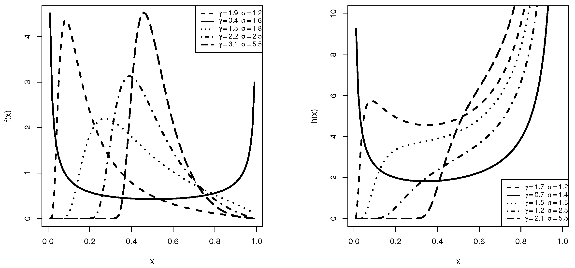
where and . The main purpose of the ULL lifetime model order is to model the educational measurements as well as other real data sets supported on the unit interval; see Korkmaz and Korkmaz [16] for additional details. Korkmaz et al. [17] investigated six classical estimation methods for the ULL model using the complete sample. Taking several selections of and , Figure 1 indicates that the density in (2) can take different shapes, including unimodal and U shape. On the other hand, the hazard rate in (5) can be increasing, bathtub, or N-shaped. Figure 1 shows that the ULL model’s varied density and hazard rate shapes make it highly flexible on the unit interval.
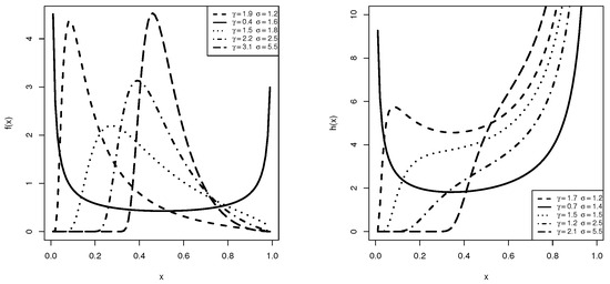
Figure 1.
Density (left) and Hazard rate (right) shapes of the ULL distribution.
We are motivated to complete the current work for the following three reasons:
- The superiority of the ULL model in fitting real data sets compared to several competing models, such as the beta and Kumaraswamy models, among others, is demonstrated later in the real data section.
- To the best of our knowledge, this is the first investigation of the estimations of the ULL distribution under censorship plans. So we consider the IT2-APC scheme, which generalizes some common censoring plans such as Type-II censoring, T2-PC, and AT2-PC schemes. As a result, the estimations employing these schemes can be directly deduced from the findings of this study.
- It is critical to understand the appropriate estimation approach for the ULL distribution and which PSP provides more information about the unknown parameters.
Before progressing further, we refer to , RF and HRF as the unknown parameters. Considering the flexibility of the ULL model and the efficiency of the IT2-APC scheme, this paper has three specific objectives, as listed below:
- Obtaining the traditional and Bayesian estimations of the unknown parameters. Employing the asymptotic properties (APs) of the maximum likelihood estimates (MLEs), the traditional maximum likelihood (ML) approach is taken into consideration in order to derive the approximate confidence intervals (ACIs) in addition to the MLEs. The squared error loss function with the Markov chain Monte Carlo (MCMC) method was then used to obtain the Bayesian estimates. Additionally, the highest posterior density (HPD) ranges are calculated.
- Examining the effectiveness of the various point and interval estimations, it is worth mentioning that assessing the different estimations theoretically is more complex. For this reason, we employ simulations to accomplish this goal. Furthermore, we prove the validity of the ULL model and the suitability of the suggested techniques through the examination of two environmental and engineering actual data sets.
- Researching the issue of choosing the best PSP for the ULL model when IT2-APC data are available. This is conducted using four precision standards. By analyzing the two given genuine data sets, these standards are numerically compared.
The remaining sections of this work are arranged as follows: Section 2 covers the classical estimation to obtain the MLEs and ACIs using the APs for various parameters. The Bayesian estimation, including prior information, posterior distribution and point and HPD interval estimations, is studied in Section 3. Section 4 presents the simulation design and simulation results based on several PSP, n, m and time boundary circumstances. In Section 5, two real environmental and engineering data sets are examined to demonstrate the effectiveness of the ULL model and the feasibility of the suggested approaches. Section 6 presents the PSP selection process as well as a comparative analysis of the various criteria that were considered. A few conclusions are presented in Section 7.
2. Likelihood Methodology
The ML estimation methodology is widely used for parameter estimation for statistical models. The ML estimation of the ULL parameters, including RF and HRF, is discussed in this part. The estimation is employed via an IT2-APC sample and PSP . Both point and interval estimates of the specified quantities are taken into consideration in this section.
2.1. Point Estimation
Considering the observable IT2-APC sample , the joint LF supplied by (1) with the PDF provided by (2), as well as the CDF in (3), can be used to write the LF of as follows, after omitting the constant term,
where
The log-LF of (6) is
The solution of the next two normal equations provides the MLEs of and , shown by and , respectively,
and
where
and
with and . Given the nonlinear functions in (8) and (9), it is evident that the MLEs cannot be determined explicitly. To find a solution to this challenge, some numerical techniques can be implemented to obtain the necessary estimates and . The invariance trait of the MLEs can be applied to find the MLEs of RF and HRF, at a given time t, by changing the genuine parameters in (4) and (5) with their MLEs, respectively, as
and
2.2. Interval Estimation of and
The ACIs of and can be created using the APs of the MLEs. Obtaining the variance-covariance matrix, denoted by , is the first step towards achieving this. However, we can approximate the necessary variance-covariance matrix by inverting the observed Fisher information matrix, as a result of the intricate formulations of the Fisher information matrix. Therefore, the approximate variance covariance matrix can be expressed as
where and
and
where
and
with , and .
The asymptotic distribution of is known to be a bivariate normal distribution with a mean of zero and an estimated variance-covariance matrix as displayed in (10), as per the APs of the MLEs. Now, at a confidence level , one can compute the required ACIs of and , respectively, as
where the standard normal distribution is used to determine .
2.3. Interval Estimation of RF and HRF
One of the problems statisticians face when developing an estimator of any function of unknown parameters is figuring out the variance of the estimator. This variance is necessary for confidence interval estimation and/or hypothesis testing. To obtain the variance of an estimator, statisticians use a procedure called the delta method, which essentially involves approximating the more complex function with a linear function that can be obtained using calculus techniques; see, for more detail, Greene [18] and Alevizakos and Koukouvinos [19]. In our case, we employ the delta method to approximate the variances of the MLEs of RF and HRF in order to obtain the ACIs of and . Let and be two vectors defined as
where
and
Therefore, one can calculate the approximate estimates of the variances of the estimators of and , respectively, as given below
Then, the ACIs for and are, as follows
3. Bayesian Methodology
This section of the paper focuses on finding Bayes estimations for the unknown parameters, RF and HRF, providing point and HPD credible interval estimates. The Bayesian method not only offers an alternative analysis but also uses informed priori densities to incorporate historical data on the parameters. Uncertainty about this knowledge is taken into account when considering noninformative priori. The Bayesian methodology uses the posterior marginal distributions to gain knowledge about the model parameters. Notably, the squared error loss function serves as the foundation for the Bayes estimations in this paper, while any other loss function can be used with ease.
3.1. Prior and Posterior Distributions
The prior distribution is a crucial component in Bayesian estimation, as it represents what is currently known about the unknown parameters. It is evident that the unknown parameters and do not have any conjugate priors. In addition, it is not easy to compute the Jeffreys prior due to the complex form of the variance-covariance matrix. We therefore presume that and have gamma prior distributions and are independent. The gamma (G) prior is chosen because of its adaptability, particularly in computational tasks. The parameter is assumed to follow . On the other hand, for , we use the three-parameter G distribution with a location parameter equal to one using the same way by Nassar et al. [20], i.e., . It should be noted that all hype-parameter values are nonnegative. Using these assumptions, the joint prior can be written as
where . The joint posterior distribution of the unknown parameters can be determined by merging the data from observations produced by the LF, as provided by (6), with the prior information that is already known, as supplied by the joint prior distribution in (11), as follows
where
The posterior mean of any parametric function, say , can be used to obtain the Bayes estimator by using the squared error loss function. Let denote the Bayes estimator of . Then, from (12), can be derived as
The ratio of integrals in (13) results in the inability to obtain the Bayes estimator in a closed form, as anticipated. We suggest using the MCMC technique to overcome this issue to obtain the required Bayes estimates as well as the HPD credible intervals. The next section discusses this topic. It is worth mentioning that another method to calculate the ratio of the integrals in Equation (13) is through a numerical integration. In Bayesian estimation, MCMC methods are commonly preferred over numerical integration for various reasons. This preference is particularly strong when dealing with models that involve two or more parameters and a complex censoring plan.
3.2. MCMC, Bayes Estimates and HPD Intervals
Employing the MCMC technique allows sampling from the posterior distribution to compute relevant posterior values. As with other Monte Carlo techniques, the MCMC makes use of repeated random sampling to make use of the law of large numbers. Partitioning the joint posterior distribution into full conditional distributions for each model parameter is required when using this technique; colorredsee the work of Noii et al. [21] for more detail about the MCMC methods. To gain the necessary estimates, a sample must be taken from each of these conditional distributions. For the parameters and , the full conditional distributions are provided, respectively, by
and
It is important to determine whether or not the full conditional distributions fit into any well-known distributions before applying the MCMC approach. Choosing which MCMC algorithm to utilize is a crucial stage in this process. As we can observe, there is no well-known distribution that can be used to describe the distributions in (14) and (15). In this circumstance, the Metropolis–Hastings (M-H) method is appropriate for obtaining the required samples from and . Following the next steps, we can use the M-H process with a normal proposal distribution (NPD) to collect the necessary samples.
- Step 1.
- Set .
- Step 2.
- Put .
- Step 3.
- Use NPD and the M-H steps to simulate from (14).
- Step 4.
- Based on NPD and the M-H steps, generate from (15).
- Step 5.
- Use to estimate pute the RF and HRF as and .
- Step 6.
- Put .
- Step 7.
- Redo steps 3 to 6 and M replications to obtain
It is crucial to eliminate the impact of the initial guesses while applying the MCMC technique. Removing the initial B replications as a burn-in phase will accomplish this. The Bayes estimate for any of the four parameters in this instance, let us say , can be acquired, as shown below
By sorting the acquired as , the HPD credible interval of can be computed accordingly
with , such that
where the greatest integer that is either smaller than or equal to is found to be .
4. Numerical Evaluations
This part establishes Monte-Carlo simulations to observe how well our estimates of , , , and from earlier sections work.
4.1. Simulation Scenarios
We constructed one thousand samples from in order to assess the relative performance of several obtained estimators for , , , and . At , the true value of () is taken as (0.49272, 1.93743). To evaluate the effectiveness of the proposed estimators under different conditions, Table 2 displays various combinations of (threshold times), n(full sample size), m(full failure size), and (progressive pattern). Additionally, to show the effects of the removal patterns, five designs of are utilized, namely: L (left), M (middle), R (right), D (doubly), and U (uniformly) censoring fashions. For example, censoring () means 1 repeats 20 times. To show how the chosen times affect the estimates, for , we also consider two different options for and . Different options of m are also determined as failure percentages (FPs) out of each n, such as %.
Table 2.
Testing scenarios performed in the Monte Carlo study.
To draw an IT2-APC sample, after assigning the values of , , and , perform the next steps:
- Step 1.
- Fix the actual values of and .
- Step 2.
- Obtain a T2-PC sample as:
- a.
- Simulate an uniform sample denoted as ().
- b.
- Set .
- c.
- Set for .
- d.
- Obtain a T2-PC sample from as .
- Step 3.
- Find at , and ignore .
- Step 4.
- Find the first order statistics (say ) from a truncated distribution with sample size .
- Step 5.
- Obtain an IT2-APC sample case as follows:
- a.
- Case-1: If ; stop the test at .
- b.
- Case-2: If ; stop the test at .
- c.
- Case-3: If ; stop the test at .
Upon gathering the desired 1000 IT2-APC samples, we install two suggested packages using the 4.2.2 programming software:
- The ‘’ tool to perform the classical estimates developed by Henningsen and Toomet [22].
- The ‘’ tool, developed by Plummer et al. [23], to perform the Bayes estimates.
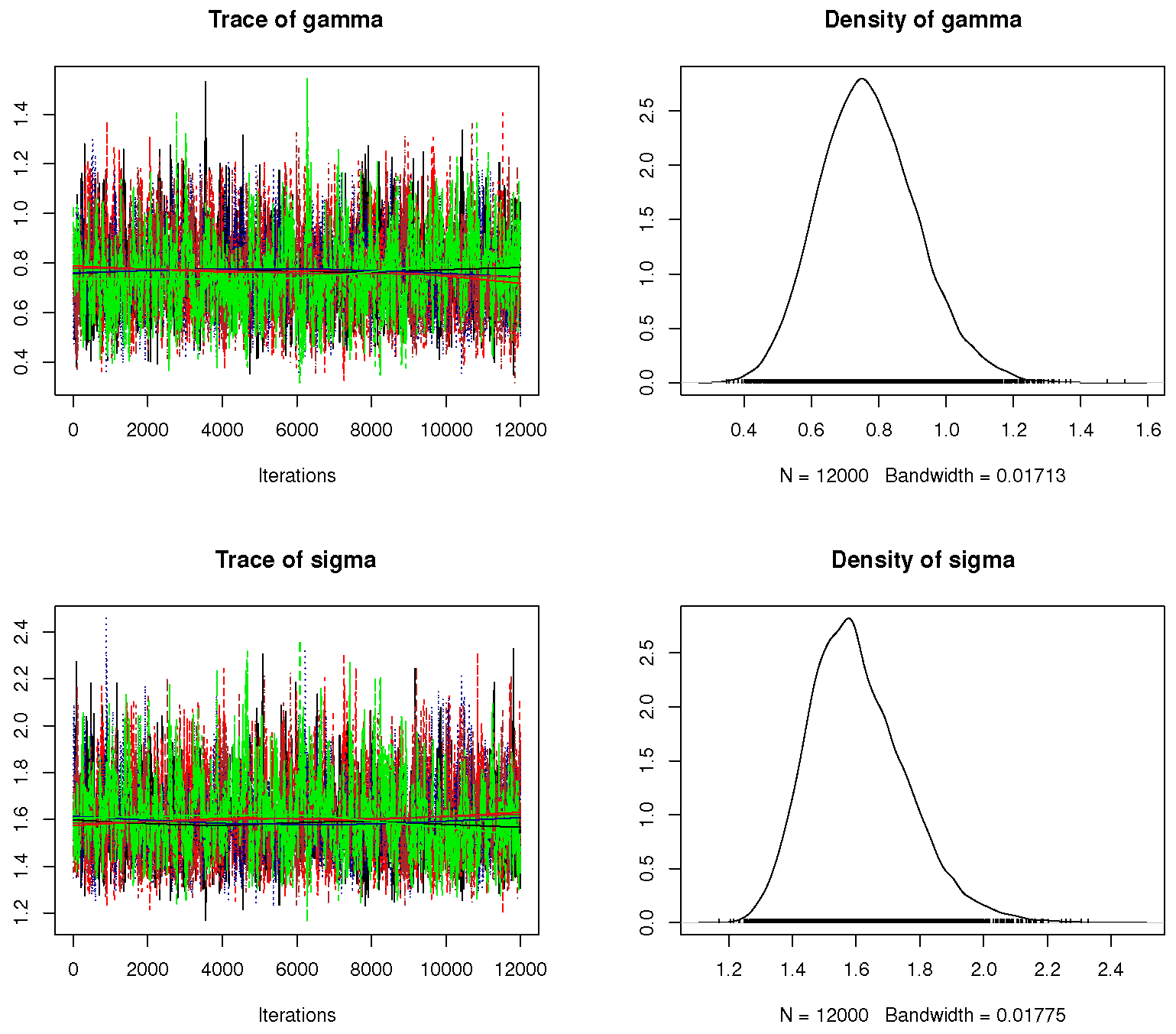
We decline the first 2000 iterations (out of 12,000) as a “burn-in” period, under the M–H steps. The Bayes–MCMC estimates and 95% HPD intervals are then computed. The Bayes inferences are performed using two informative sets of , referred to as Pr.A: (7.5, 5, 10, 10) and Pr.B: (15, 10, 20, 20), which are compatible with both prior-mean and prior-variance criteria. The suggested values of for are allocated so that the sample mean of or is achieved by the prior mean. In order to obtain an appropriate sample from the objective posterior distribution in MCMC assessments, we must ensure the convergence of the generated chains. Four convergence operators, (i) the auto-correlation function (ACF), (ii) Trace, (iii) Brooks–Gelman–Rubin (BGR) diagnostic, and (iv) Trace thinning-based are utilized to achieve this goal (here, we used every fifth point). When , , , , and Pr.A. are applied, these measures are carried out. Figure 2a demonstrates that there is a strong correlation between the lag in each chain and the autocorrelation of each parameter. This suggests that the simulated chains are highly mixed together. Figure 2b shows that the variance within the Markovian chains and the variance between them are not significantly different. This also shows that the size of the burn-in sample is a good way to get rid of the effects of the starting points. Figure 2c displays that the simulated chains are substantially mixed. All Markovian chains, shown in Figure 3, seem to explore the same region of the actual parameter values of or , which is a good sign. These chains support the same facts displayed in Figure 2c, which states that the simulated chains are substantially mixed. As a result, the computed point (or interval) estimates of , , , and are reliable and good. The same findings are observed when using Pr.B.
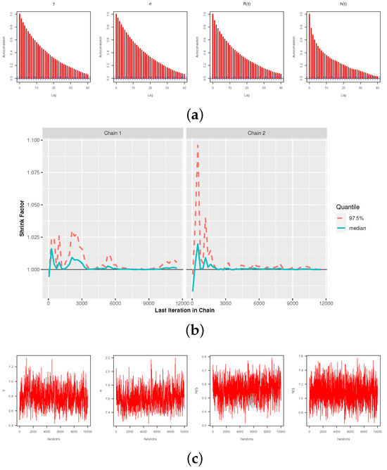
Figure 2.
The MCMC visuals of , , , and with (a) ACF, (b) BGR and (c) Trace, for Monte Carlo simulation.
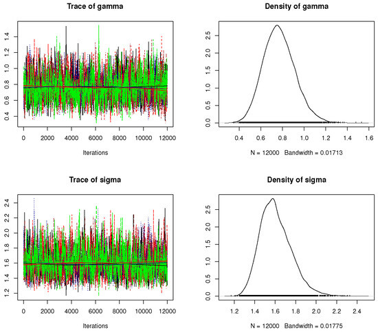
Figure 3.
Trace (left panel) and density (right panel) plots and in Monte Carlo simulation.
From the acquired estimates, say for the parameter as an example, we obtain some statistical measures, namely the average estimates (AEs), root mean squared-errors (RMSEs), mean absolute biases (MABs), average confidence widths (ACWs) and coverage percentages (CPs). The expressions of these measures are, respectively, given by
and
where where is the estimate of at ith sample, denotes the indicator operator and denote the (lower,upper) limits of ACI (or HPD) interval of .
4.2. Simulation Results
All outcomes of the simulation of , , , and are displayed in the supplementary file. In Table 3 and Table 4, for brevity, the point and interval estimations of , , , and when n[FP%] = 40[50%] are presented. Considering the lowest values of RMSE, MAB, and ACW along with the greatest values of CP, we list the following observations:
Table 3.
Av.Es (1st column), RMSEs (2nd column) and MABs (3rd column) of , , , and when n[FP%] = 40[50%].
Table 4.
The ACWs (1st column) and CPs (2nd column) of 95% ACI/HPD intervals of , , , and when n[FP%] = 40[50%].
- The most significant finding is that the provided , , , or estimates are accurate.
- As n(or m) grows, all estimates of , , , or behave better. When decreases, a similar conclusion is offered.
- As for increase, all offered estimates of , , , or perform satisfactorily.
- Due to the additional information we already have about and , the Bayes estimates of all parameters are more accurate than other estimates, as expected. The same thing is noticed when comparing the HPD credible intervals with the ACIs.
- By changing the hyperparameters from Pr.A to Pr.B, we can observe the same conclusion that the Bayes point estimates and HPD credible intervals outperform those based on the ML method.
- Because the variance of Pr.B is smaller than the variance of Pr.A, all the Bayes estimations based on Pr.B are more accurate than others.
- Comparing the proposed schemes L, M, R, D, and U, it is observed that all results of , , , or behave superiorly based on censoring-U ‘uniformly’ (next, censoring-D ‘doubly’) than others.
- So, in order to obtain accurate results for any parameter of life, the practitioner doing the experiment needs to make the experiment last for as long as possible if and only if the experiment cost is enough.
- In summary, when dealing with data gathered using an IT2-APC process, it is recommended to use the Bayes’ framework with M-H sampling to estimate the ULL parameters ( and ) or reliability features ( and ).
5. Real-Life Applications
This part illustrates two examples that show how to use the suggested methods in real-life situations. These examples use real data from the fields of environmental science and engineering.
5.1. Environmental Data Analysis
In this application, we will study a set of data that shows the maximum (highest) flood level (MFL) of the Susquehanna River in Harrisburg, Pennsylvania. The data are measured in millions of cubic feet per second; see Table 5. Dumonceaux and Antle [24] presented this information, which was later assessed by Dey et al. [25].
Table 5.
The MFL data of Susquehanna River.
To highlight the superiority of the ULL lifetime model based on the full MFL data, we will compare it with seven other models in the literature, named:
- (1)
- unit-Birnbaum-Saunders (UBS) by Mazucheli et al. [26];
- (2)
- unit-Gompertz (UGom) by Mazucheli et al. [27];
- (3)
- unit-Weibull (UW) by Mazucheli et al. [28];
- (4)
- unit-gamma (UG) by Mazucheli et al. [29];
- (5)
- Topp-Leone (TL) by Topp and Leone [30];
- (6)
- Kumaraswamy (Kum) by Mitnik and Baek [31];
- (7)
- Beta by Gupta and Nadarajah [32].
To specify the best model among the ULL and its competitors, we consider the following metrics:
- (1)
- Estimated log-likelihood (say ), where ;
- (2)
- Akaike information (), where ;
- (3)
- Bayesian information (), where ;
- (4)
- Consistent Akaike information (), where ;
- (5)
- Hannan-Quinn information (), where ;
- (6)
- The Kolmogorov–Smirnov () statistic is defined aswhere and , such as its P-value being given by
- (7)
- Anderson–Darling () statistic is defined aswhere , is the cumulative of the standard normal distribution, s and denote the standard deviation and mean data points. The P-value of statistic is provided bywhere is a modified statistic; see Table 4.9 in Stephens [33].
- (8)
- Cramér-von Mises () statistic is defined assuch as its P-value is given bywhere is a modified statistic; see Table 4.9 in Stephens [33].
Except for the highest P-values, the best model is the one that yields the lowest values for all goodness of fit statistics. Table 6 shows the MLEs (with standard errors (St.Ers)) of and for the ULL or its rivals based on the full MFL data, together with the fitted values of all the criteria that were previously mentioned. Because the ULL lifetime model yields the greatest P-values from the , , or test and the lowest values for all other metrics, it is the best option among the fitted models, as presented in Table 6.
Table 6.
Fitting outputs of the ULL and its competitive models from MFL data.
We also presented five graphical demonstrations of our fitting, namely:
- (1)
- Probability–probability (PP); see Figure 4a;
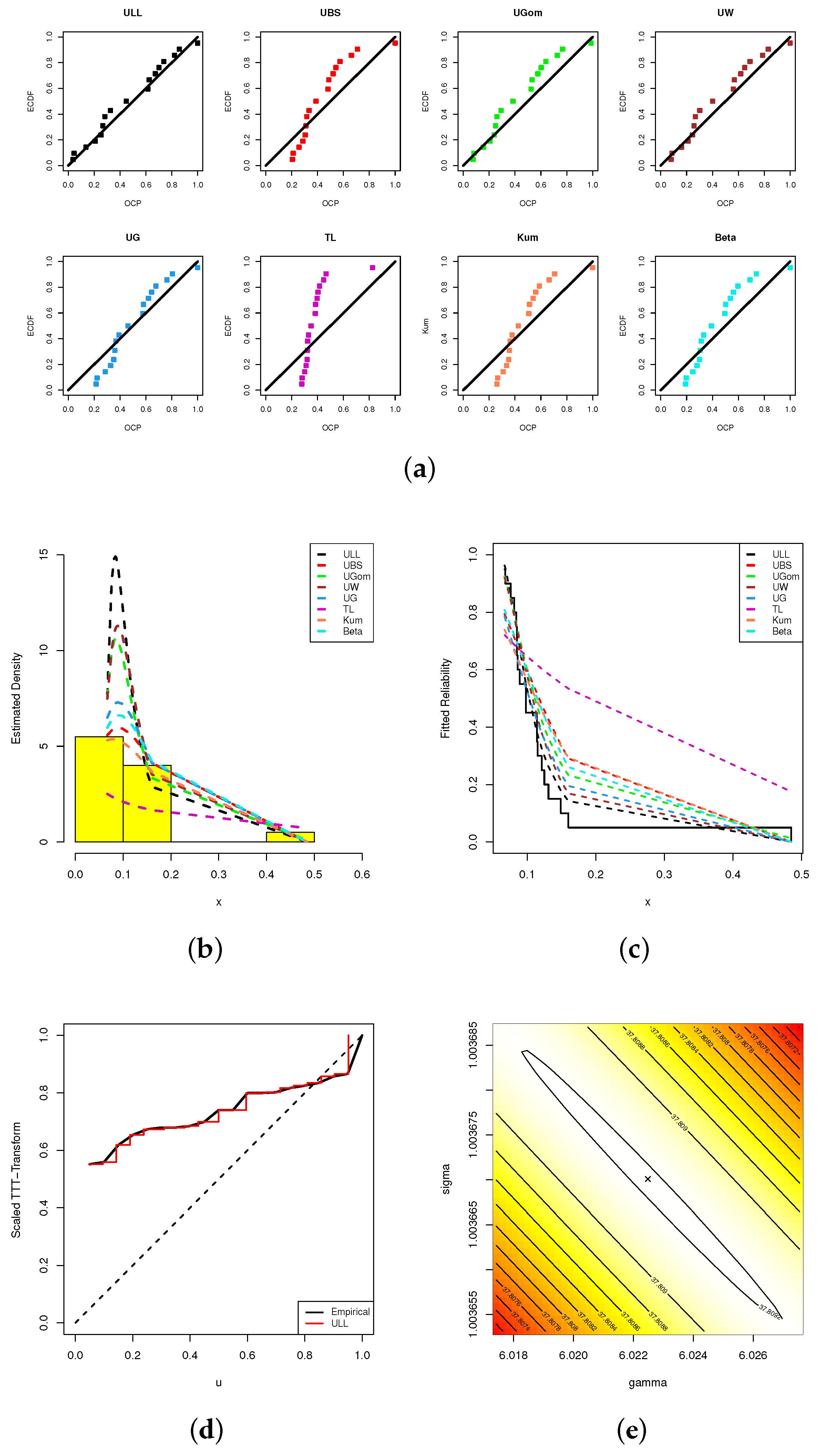
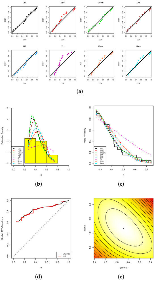 Figure 4. Fitting visualizations, including (a) PP, (b) Histogram, (c) Reliability, (d) TTT, and (e) Contour, from MFL data.
 - (2)
- Data histograms with fitted density lines; see Figure 4b;
- (3)
- Fitted reliability lines; see Figure 4c;
- (4)
- Scaled–TTT transform; see Figure 4d;
- (5)
- Contour; see Figure 4e.
Figure 4a shows that the probability dots closely match the theoretical probability line. The fitted ULL density line in Figure 4b accurately captures the MFL data histograms. The fitted reliability line of the ULL model in Figure 4c is a better match for the empirical reliability line compared to other models. Figure 4d also illustrates that the MFL data set has an increasing failure rate, which confirms the same information shown in Figure 1. Additionally, Figure 4e displays that the estimated values of and exist and are unique. Henceforth, we suggest using and as starting points to run any additional computations.
To examine the proposed inference methodologies, from Table 5, for a fixed FP = 50% and several choices of and , different IT2-APC samples of size are created; see Table 7. For each data set in Table 7, the MLE and Bayes’ MCMC estimate (along with their St.Ers) as well as the 95% ACI/HPD interval estimates (along with their interval widths (IWs)) of , , , or (at ) are obtained; see Table 8. After repeating the MCMC sampler 50,000 times and removing the first 10,000 times (burn-in), the acquired Bayes and HPD interval estimators are evaluated using improper gamma priors. For computational logic, we set for equal to 0.001. The results reported in Table 8 indicate that the offered point and HPD interval estimates using the Bayesian approach outperform the classical ones in terms of minimum St.Ers and IWs.
Table 7.
Artificial IT2-APC samples from MFL data.
Table 8.
Estimates of , , , and from MFL data.
To show that the acquired MLEs of and exist and are unique, we look at their profile log-likelihood functions. Please refer to the supplementary file. They demonstrate, based on all samples produced from MFL, that the estimated values of or exist and are unique.
Both density and trace plots of , , , and for each data set mentioned in Table 7 are shown in the supplementary file to demonstrate the convergence of MCMC iterations. These plots indicate that the MCMC approach yields satisfactory results. The recommended number of samples to be discarded is sufficient to mitigate the impact of the recommended beginning values. In these plots, the dotted line represents the 95% HPD interval boundaries, and the solid line represents the Bayes estimate. Additionally, the findings show that while the estimated values of are negatively skewed, the values of , , and are almost symmetrical. We extracted several characteristics from the remaining 40,000 MCMC variates of , , , and , including mean, first quartile, median, third quartile, mode, standard deviation (St.Dv.), and skewness (Skew.), which are also provided in the supplementary file.
5.2. Engineering Data Analysis
This application examines a collection of data indicating the duration of twenty mechanical components (MCs) until they cease functioning. This data set was first provided by Murthy et al. [34]. In Table 9, the MCs data are provided.
Table 9.
Failure times of 20 mechanical components.
Before considering the estimations, we have two concerns: (i) what is the validity of ULL for MCs data, and (ii) what is the superiority of the ULL model compared to the other models discussed in Section 5.1? Table 10 presents the MLEs (with their St.Ers) of and in addition to all fitted criteria (including: , , , , , (p-value), (p-value), and (p-value)). The findings reported in Table 10 show that the ULL distribution provides a good fit for the MCs data set compared to others.
Table 10.
Fitting outputs of the ULL and its competitive models from MCs’ data.
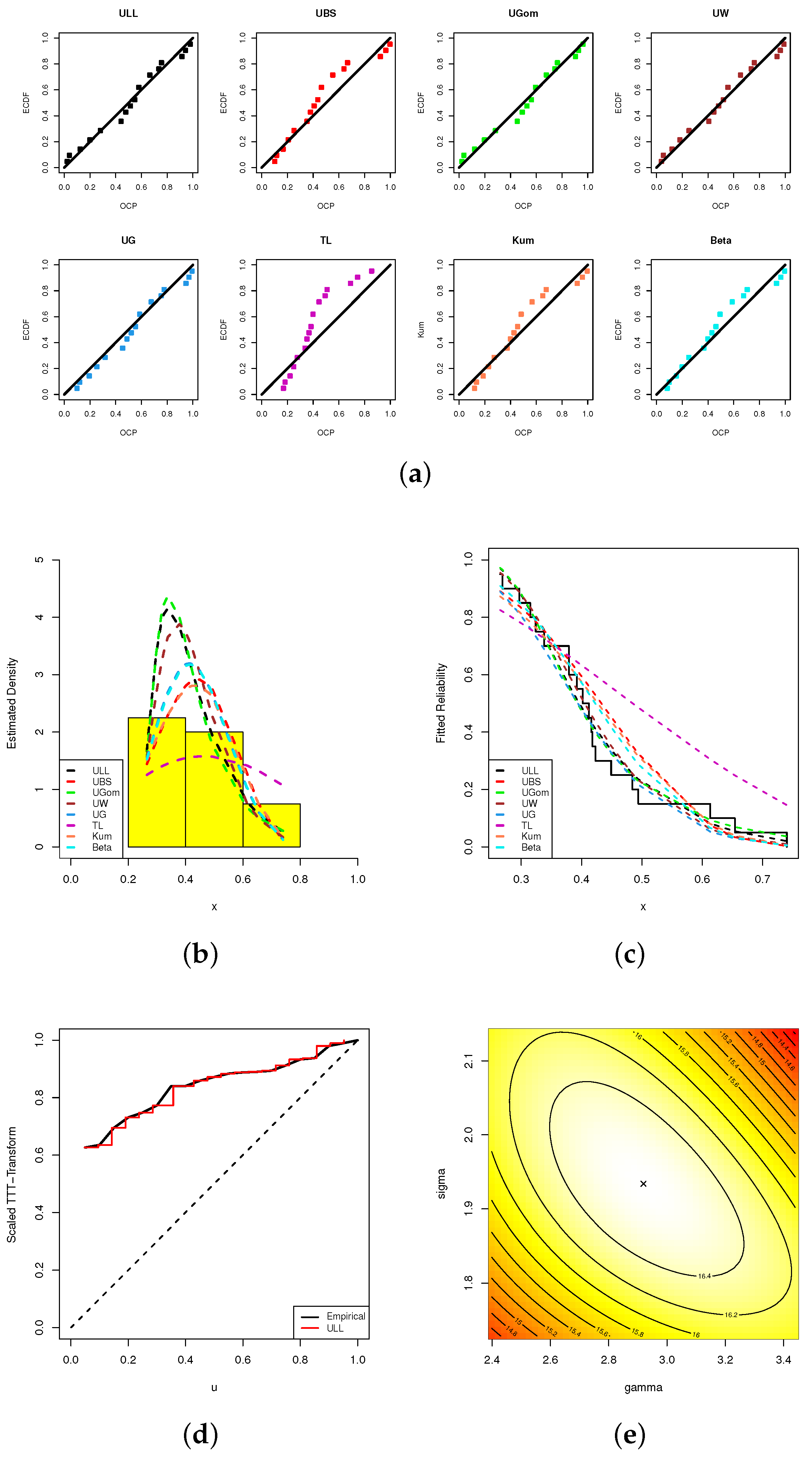
Following the same graphical tools depicted in Figure 4, Figure 5a shows that the dots representing probability closely match the line representing the theoretical probability more than others. The estimated ULL density line in Figure 5b shows that the ULL distribution matches better with the histograms of the MCs data than others. The ULL model’s reliability line in Figure 5c matches the real-life reliability line better than other models. The information depicted in Figure 5d is reinforced by the observation that the MCs’ data set exhibits an increasing failure rate. Additionally, it can be observed from Figure 5e that the estimated values exist and are unique for both and . We thus consider the estimates and as initial guess points to perform any additional computations based on MCs’ data.
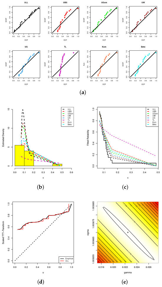
Figure 5.
Fitting visualizations, including (a) PP, (b) Histogram, (c) Reliability, (d) TTT, and (e) Contour, from MCs data.
Just like our scenarios discussed in Section 5.1, from the complete MCs data, we shall evaluate all offered estimators of , , , and (at ). From Table 11, by taking , based on some choices of and , five various IT2-APC samples are generated; see Table 9. Frequentist and Bayes’ MCMC estimates (with their St.Ers) of , , , and are calculated; see Table 12. Additionally, in Table 12, two-sided 95% ACI/HPD interval estimates (with their IWs) of the same unknown parameters are reported. From Table 12, one can observe that the Bayesian-based point and HPD interval estimates are superior to the conventional estimates in terms of minimum St.Ers and IWs.
Table 11.
Artificial IT2-APC samples from MCs data.
Table 12.
Estimates of , , , and from MCs’ data.
The profile log-likelihood functions of and (shown in the Supplementary File) indicate the existence and uniqueness of the estimates of and . We examine the trace plots of the variables , , , and to observe whether the MCMC algorithm is operating efficiently. All trace plots illustrate that applying the final 40,000 MCMC iterations is effective and produces good results for all the unknown values. Additionally, the vital statistics of , , , and (presented in the supplementary file) demonstrate that although the computed estimates for are negatively skewed, those for , , or are fairly symmetrical.
6. Optimum Progressive Scenario
The goal during reliability trials is to assess and decide upon the optimal (best) progressive censoring from a group of available options. So, choosing the best progressive design has been a topic of interest in statistics. For more information, one can refer to Ng et al. [35], Pradhan and Kundu [36], and other researchers have also studied this topic. To determine the best fashion of progressive censoring among others to gather information about unknown parameters under consideration, Table 1 lists different criteria to help us choose the best progressive plan.
Our objective for Crit[1] is to maximize the values of the numbers found on the main diagonal of the estimated Fisher information. In the same way, considering both Crit[i] for , we aim to reduce both trace and determinant of the approximated OVC matrix, respectively. Furthermore, criterion Crit[4] helps to decrease the variance of log-MLE of the qth quantile, denoted by , such as
where the delta method is reconsidered here to evaluate . Subsequently, to choose the best progressive design, one needs to find the progressive pattern that has the smallest values for Crit[i] for , and the largest value for Crit[1].
6.1. Optimum Progressive Using Environmental Data
To pick the optimum progressive scenario from the given MFL data, all optimum criteria reported in Table 13 are evaluated through the acquired MLEs and (which are provided in Table 8). In order to ascertain the optimal progressive design among the suggested schemes utilized in samples A, B, C, D, and E, Table 14 presents the optimum Crit[i] for derived from the MFL data.
Table 13.
Criteria of the best progressive censoring.
Table 14.
Optimum progressive plans from MFL data.
Results in Table 14 indicate that:
- Via Crit[i] for ; the R-censoring (in Sample C) is the optimum than others.
- Via Crit[2]; the U-censoring (in Sample E) is optimal one vs. others.
6.2. Optimum Progressive Using Engineering Data
Using the MCs’ data, to find the optimum progressive pattern, all optimum criteria reported in Table 13 are evaluated through the acquired MLEs and (which are provided in Table 12). In Table 15, the fitted optimum Crit[i] for , from the MCs’ data, are provided.
Table 15.
Optimum progressive plans from MCs’ data.
Results in Table 15 indicated that:
- Via Crit[1]; the L-censoring (in Sample A) is the optimal one vs. others.
- Via Crit[2]; the U-censoring (in Sample E) is the optimal one vs. others.
- Via Crit[i] for ; the R-censoring (in Sample C) is the optimal one vs. others.
The best progressive designs, based on the highest flood level and data on mechanical parts, support the same conclusions mentioned in Section 2. In simpler terms, based on the analysis conducted in the environment and engineering fields, we can say that the suggested methods work well on real-world data and provide a good understanding of the lifetime model. These findings are limited by the use of the ULL model and the IT2-APC plan, and they cannot be generalised to other lifetime models or censorship techniques.
7. Concluding Remarks
This study provided a range of statistical inference methodologies covering the estimation of the unit log-log model, including the model parameters and some reliability benchmarks in the context of improved adaptive progressively Type-II censored data. The work in this paper is divided into three parts. The first part derives the point and interval estimations using classical and Bayesian approaches. The maximum likelihood and Bayesian estimation via squared error loss functions are employed for this purpose. The second part includes the numerical comparison between the various estimates. A simulation study under several situations is considered to compare the various point and interval estimations using some statistical standards, including the mean square error and coverage probability. Two genuine data sets from various domains are analyzed from a practical perspective to demonstrate the applicability of the proposed methodologies. The primary deduction drawn from the second part is that the Bayesian method outperforms the conventional method. Furthermore, the two applications demonstrated how adaptable the unit log-log model is as well as how it can yield better results than certain well-known models. The final part explored the selection of the appropriate progressive censoring approach. For this, four precision criteria are considered. We applied the given criteria to the real data sets examined in the real data section to demonstrate their significance. In future work, it is important to compare the proposed analytical methods with some other methods, such as the product of spacings and E-Bayesian methods.
Supplementary Materials
The following supporting information can be downloaded at: https://www.mdpi.com/article/10.3390/axioms13030152/s1, Table S1: Av.Es (1st column), RMSEs (2nd column) and MABs (3rd column) of when ; Table S2: Av.Es (1st column), RMSEs (2nd column) and MABs (3rd column) of when ; Table S3: Av.Es (1st column), RMSEs (2nd column) and MABs (3rd column) of when ; Table S4: Av.Es (1st column), RMSEs (2nd column) and MABs (3rd column) of when ; Table S5: Av.Es (1st column), RMSEs (2nd column) and MABs (3rd column) of when ; Table S6: Av.Es (1st column), RMSEs (2nd column) and MABs (3rd column) of when ; Table S7: Av.Es (1st column), RMSEs (2nd column) and MABs (3rd column) of when ; Table S8: Av.Es (1st column), RMSEs (2nd column) and MABs (3rd column) of when ; Table S9: The ACWs (1st column) and CPs (2nd column) of 95% ACI/HPD intervals of when ; Table S10: The ACWs (1st column) and CPs (2nd column) of 95% ACI/HPD intervals of when ; Table S11: The ACWs (1st column) and CPs (2nd column) of 95% ACI/HPD intervals of when ; Table S12: The ACWs (1st column) and CPs (2nd column) of 95% ACI/HPD intervals of when ; Table S13: The ACWs (1st column) and CPs (2nd column) of 95% ACI/HPD intervals of when ; Table S14: The ACWs (1st column) and CPs (2nd column) of 95% ACI/HPD intervals of when ; Table S15: The ACWs (1st column) and CPs (2nd column) of 95% ACI/HPD intervals of when ; Table S16: The ACWs (1st column) and CPs (2nd column) of 95% ACI/HPD intervals of when ; Table S17: Properties of , , , and from MFL data; Table S18: Properties of , , , and from MCs data; Figure S1: Profile log-likelihoods of (left) and (right) from MFL data; Figure S2: Density (left) and Trace (right) plots of , , , and from MFL data; Figure S3: Profile log-likelihoods of (left) and (right) from MFL data; and Figure S4: Density (left) and Trace (right) plots of , , , and from MCs data.
Author Contributions
Methodology, R.A. and M.N.; Funding acquisition, R.A.; Software, A.E.; Supervision, M.N.; Writing—original draft, R.A. and M.N.; Writing—review and editing, A.E. and M.N. All authors have read and agreed to the published version of the manuscript.
Funding
This research was funded by Princess Nourah bint Abdulrahman University Researchers Supporting Project number (PNURSP2024R50), Princess Nourah bint Abdulrahman University, Riyadh, Saudi Arabia.
Data Availability Statement
The authors confirm that the data supporting the findings of this study are available within the article.
Acknowledgments
The authors would also like to express thanks to the Editor-in-Chief and three anonymous referees for their constructive comments and suggestions, which significantly improved the paper. Princess Nourah bint Abdulrahman University Researchers Supporting Project number (PNURSP2024R50), Princess Nourah bint Abdulrahman University, Riyadh, Saudi Arabia.
Conflicts of Interest
The authors declare no conflicts of interest.
References
- Balakrishnan, N.; Aggarwala, R. Progressive Censoring: Theory, Methods, and Applications; Springer Science & Business Media: Berlin, Germany, 2000. [Google Scholar]
- Ng, H.K.T.; Kundu, D.; Chan, P.S. Statistical analysis of exponential lifetimes under an adaptive Type-II progressive censoring scheme. Nav. Res. Logist. 2009, 56, 687–698. [Google Scholar] [CrossRef]
- Kundu, D.; Joarder, A. Analysis of Type-II progressively hybrid censored data. Comput. Stat. Data Anal. 2006, 50, 2509–2528. [Google Scholar] [CrossRef]
- Sobhi, M.M.A.; Soliman, A.A. Estimation for the exponentiated Weibull model with adaptive Type-II progressive censored schemes. Appl. Math. Model. 2016, 40, 1180–1192. [Google Scholar] [CrossRef]
- Chen, S.; Gui, W. Statistical analysis of a lifetime distribution with a bathtub-shaped failure rate function under adaptive progressive type-II censoring. Mathematics 2020, 8, 670. [Google Scholar] [CrossRef]
- Panahi, H.; Moradi, N. Estimation of the inverted exponentiated Rayleigh distribution based on adaptive Type II progressive hybrid censored sample. J. Comput. Appl. Math. 2020, 364, 112345. [Google Scholar] [CrossRef]
- Kohansal, A.; Shoaee, S. Bayesian and classical estimation of reliability in a multicomponent stress-strength model under adaptive hybrid progressive censored data. Stat. Pap. 2021, 62, 309–359. [Google Scholar] [CrossRef]
- Du, Y.; Gui, W. Statistical inference of adaptive type II progressive hybrid censored data with dependent competing risks under bivariate exponential distribution. J. Appl. Stat. 2022, 49, 3120–3140. [Google Scholar] [CrossRef] [PubMed]
- Alotaibi, R.; Elshahhat, A.; Rezk, H.; Nassar, M. Inferences for Alpha Power Exponential Distribution Using Adaptive Progressively Type-II Hybrid Censored Data with Applications. Symmetry 2022, 14, 651. [Google Scholar] [CrossRef]
- Yan, W.; Li, P.; Yu, Y. Statistical inference for the reliability of Burr-XII distribution under improved adaptive Type-II progressive censoring. Appl. Math. Model. 2021, 95, 38–52. [Google Scholar] [CrossRef]
- Nassar, M.; Elshahhat, A. Estimation procedures and optimal censoring schemes for an improved adaptive progressively type-II censored Weibull distribution. J. Appl. Stat. 2023, 1–25. [Google Scholar] [CrossRef]
- Elshahhat, A.; Nassar, M. Inference of improved adaptive progressively censored competing risks data for Weibull lifetime models. Stat. Pap. 2023, 1–34. [Google Scholar] [CrossRef]
- Elbatal, I.; Nassar, M.; Ben Ghorbal, A.; Diab, L.S.G.; Elshahhat, A. Reliability Analysis and Its Applications for a Newly Improved Type-II Adaptive Progressive Alpha Power Exponential Censored Sample. Symmetry 2023, 15, 2137. [Google Scholar] [CrossRef]
- Alam, F.M.A.; Nassar, M. On Entropy Estimation of Inverse Weibull Distribution under Improved Adaptive Progressively Type-II Censoring with Applications. Axioms 2023, 12, 751. [Google Scholar] [CrossRef]
- Dutta, S.; Kayal, S. Inference of a competing risks model with partially observed failure causes under improved adaptive type-II progressive censoring. Proceedings of the Institution of Mechanical Engineers. Part J. Risk Reliab. 2023, 237, 765–780. [Google Scholar]
- Korkmaz, M.Ç.; Korkmaz, Z.S. The unit log–log distribution: A new unit distribution with alternative quantile regression modeling and educational measurements applications. J. Appl. Stat. 2023, 50, 889–908. [Google Scholar] [CrossRef] [PubMed]
- Korkmaz, M.Ç.; Karakaya, K.; Akdoğan, Y.; Yener, Ü.N.A.L. Parameters Estimation for the Unit log-log Distribution. Cumhur. Sci. J. 2023, 44, 224–228. [Google Scholar] [CrossRef]
- Greene, W.H. Econometric Analysis, 4th ed.; Prentice-Hall: NewYork, NY, USA, 2000. [Google Scholar]
- Alevizakos, V.; Koukouvinos, C. An asymptotic confidence interval for the process capability index Cpm. Commun.-Stat.-Theory Methods 2019, 48, 5138–5144. [Google Scholar] [CrossRef]
- Nassar, M.; Alotaibi, R.; Elshahhat, A. Reliability Estimation of XLindley Constant-Stress Partially Accelerated Life Tests using Progressively Censored Samples. Mathematics 2023, 11, 1331. [Google Scholar] [CrossRef]
- Noii, N.; Khodadadian, A.; Ulloa, J.; Aldakheel, F.; Wick, T.; Francois, S.; Wriggers, P. Bayesian inversion with open-source codes for various one-dimensional model problems in computational mechanics. Arch. Comput. Methods Eng. 2022, 29, 4285–4318. [Google Scholar] [CrossRef]
- Henningsen, A.; Toomet, O. maxLik: A package for maximum likelihood estimation in R. Comput. Stat. 2011, 26, 443–458. [Google Scholar] [CrossRef]
- Plummer, M.; Best, N.; Cowles, K.; Vines, K. CODA: Convergence diagnosis and output analysis for MCMC. R News 2006, 6, 7–11. [Google Scholar]
- Dumonceaux, R.; Antle, C.E. Discrimination between the log-normal and the Weibull distributions. Technometrics 1973, 15, 923–926. [Google Scholar] [CrossRef]
- Dey, S.; Menezes, A.F.; Mazucheli, J. Comparison of estimation methods for unit-gamma distribution. J. Data Sci. 2019, 17, 768–801. [Google Scholar] [CrossRef]
- Mazucheli, J.; Menezes, A.F.; Dey, S. The unit-Birnbaum-Saunders distribution with applications. Chil. J. Stat. 2018, 9, 47–57. [Google Scholar]
- Mazucheli, J.; Menezes, A.F.; Dey, S. Unit-Gompertz distribution with applications. Statistica 2019, 79, 25–43. [Google Scholar]
- Mazucheli, J.; Menezes, A.F.B.; Fern, L.B.; De Oliveira, R.P.; Ghitany, M.E. The unit-Weibull distribution as an alternative to the Kumaraswamy distribution for the modeling of quantiles conditional on covariates. J. Appl. Stat. 2020, 47, 954–974. [Google Scholar] [CrossRef] [PubMed]
- Mazucheli, J.; Menezes, A.F.B.; Dey, S. Improved maximum-likelihood estimators for the parameters of the unit-gamma distribution. Commun.-Stat.-Theory Methods 2018, 47, 3767–3778. [Google Scholar] [CrossRef]
- Topp, C.W.; Leone, F.C. A family of J-shaped frequency functions. J. Am. Stat. Assoc. 1955, 50, 209–219. [Google Scholar] [CrossRef]
- Mitnik, P.A.; Baek, S. The Kumaraswamy distribution: Median-dispersion re-parameterizations for regression modeling and simulation-based estimation. Stat. Pap. 2013, 54, 177–192. [Google Scholar] [CrossRef]
- Gupta, A.K.; Nadarajah, S. Handbook of Beta Distribution and Its Applications; CRC Press: Boca Raton, FL, USA, 2004. [Google Scholar]
- Stephens, M.A. Tests based on EDF statistics. In Goodness-of-Fit Techniques; D’Agostino, R.B., Stephens, M.A., Eds.; Marcel Dekker: New York, NY, USA, 1986. [Google Scholar]
- Murthy, D.N.P.; Xie, M.; Jiang, R. Weibull Models; Wiley Series in Probability and Statistics; Wiley: Hoboken, NJ, USA, 2004. [Google Scholar]
- Ng, H.K.T.; Chan, C.S.; Balakrishnan, N. Optimal progressive censoring plans for the Weibull distribution. Technometrics 2004, 46, 470–481. [Google Scholar] [CrossRef]
- Pradhan, B.; Kundu, D. On progressively censored generalized exponential distribution. Test 2009, 18, 497–515. [Google Scholar] [CrossRef]

Disclaimer/Publisher’s Note: The statements, opinions and data contained in all publications are solely those of the individual author(s) and contributor(s) and not of MDPI and/or the editor(s). MDPI and/or the editor(s) disclaim responsibility for any injury to people or property resulting from any ideas, methods, instructions or products referred to in the content. |
© 2024 by the authors. Licensee MDPI, Basel, Switzerland. This article is an open access article distributed under the terms and conditions of the Creative Commons Attribution (CC BY) license (https://creativecommons.org/licenses/by/4.0/).