Stress–Strength Reliability Analysis for Different Distributions Using Progressive Type-II Censoring with Binomial Removal

Abstract

In the statistical literature, one of the most important subjects that is commonly used is stress–strength reliability, which is defined as $\delta =P\left[W<V\right]$, where V and W are the strength and stress random variables, respectively, and $\delta$ is reliability parameter. Type-II progressive censoring with binomial removal is used in this study to examine the inference of $\delta =P\left[W<V\right]$ for a component with strength V and being subjected to stress W. We suppose that V and W are independent random variables taken from the Burr XII distribution and the Burr III distribution, respectively, with a common shape parameter. The maximum likelihood estimator of $\delta$ is derived. The Bayes estimator of $\delta$ under the assumption of independent gamma priors is derived. To determine the Bayes estimates for squared error and linear exponential loss functions in the lack of explicit forms, the Metropolis–Hastings method was provided. Utilizing comprehensive simulations and two metrics (average of estimates and root mean squared errors), we compare these estimators. Further, an analysis is performed on two actual data sets based on breakdown times for insulating fluid between electrodes recorded under varying voltages.

1. Introduction

A growing amount of pressure has been placed on manufacturers in recent years to create high-quality goods while lowering manufacturing costs and time frames. Studying reliability is increasingly important as global competitiveness increases. Reliability estimates, prediction, and optimization are built on the pillars of lifetime testing, structural reliability, and machine maintenance. The stress–strength (SS) model is mathematically written as $\delta =P\left[W<V\right]$, where V is the strength random variable, W is the stress random variable, and $\delta$ is the reliability parameter. In this model, the probability that the system can withstand the pressures placed on it is known as the system’s reliability, or $\delta =P\left[W<V\right].$ A good illustration of both mechanical engineering and aerodynamics is the reliability of aircraft windshields. Various fields, including engineering, medicine, and the military, can employ SS models. SS reliability can provide scenarios for reliable structures such as carbon fiber, bridges, lifts, and others. The parameter $\delta$ is undoubtedly applicable in a wide range of sectors and offers more than just an SS model. It also gives a broad assessment of the differences between the two populations. For instance, in clinical investigations, we may assess the effectiveness of two treatments to compare V, the patient’s life expectancy while receiving one medicine, and W, the patient’s life expectancy when receiving a different medication. Information on more applications of this model can be found in [1]. Numerous studies on the S-S model using complete and censored samples have been conducted by [2,3,4,5,6,7,8,9,10,11,12] and others. Some recent studies concerning SS models can be found in [13,14,15,16,17,18,19].

Censored samples are used to analyze lifetime data because, in life-testing trials, one frequently runs into circumstances where it takes a long time to accumulate sufficient number of failures needed to make a meaningful judgment. In the past ten years, the Type-II progressive censoring (TII-PC) scheme has become one of the most popular censoring methods. The following is an explanation of it: Assume that n identical units will be tested, and m failures will be recorded. When the first failure occurs, $R_1$ items are randomly selected and eliminated from the ($n-1$). Similar to the first failure, $R_2$ items of the surviving objects are selected at random and eliminated, and so on. The remaining items are all suppressed at the moment of the $mth$ failure. $R=(R_1,R_2,\dots ,R_m)$ displays the TII-PC scheme. For $R=(0,0,\dots ,n-m)$ in TII-PC, Type-II censoring is obtained, and a complete sampling scheme when ($n=m$) and $(R_1=\dots =R_{m-1}=R_m=0)$. Research on the various characteristics of progressive censoring systems was provided by Balakrishnan [20] and Aggarwala and Balakrishnan [21]. The prefixes $R_1,R_2,\dots ,R_m$ are all present in this system. However, these numbers might happen at random in some real-world scenarios. According to Yuen and Tse [22], for instance, it is random and impossible to predict how many patients will withdraw from a clinical test at any given point. Additionally, even when some of the tested units have not failed, an experimenter may determine in some reliability trials that it is unsuitable or too unsafe to continue testing on some of the tested units. In these situations, the removal pattern is arbitrary at every failure (Yuen and Tse [22] and Amin [23]). This results in arbitrary removals and gradual censoring. As a result, several writers, including Wu et al. [24], Tse et al. [25], Dey and Dey [26], and Yan et al. [27], have examined the statistical inference on lifetime distributions under TII-PC with random removals.

In the literature, there is only one study regarding the parametric inference of the SS model with the stress and strength random variables belonging to the Marshall–Olkin extended Weibull family and where the observed samples are the TII-PC with fixed or random removal, as reported by Mokhlis et al. [28]. The main goal of the present work is to examine the estimate of the SS reliability parameter $\delta =P\left[W<V\right]$ when the W and V are independent random variables with distinct distributions and the observed samples are the TII-PC with binomial removal. So, we will now give a brief summary of our research.

1.

The parent distributions, Burr XII (BXII) with shape parameters $(\vartheta ,{\phi }_1)$ and Burr III (BIII) with shape parameters $(\vartheta ,{\phi }_2)$, linked to $\delta$, are described, and their significance is discussed.

2.

An explicit expression of the SS reliability parameter $\delta$ is derived, when V and W are independent random variables following BXII $(\vartheta ,{\phi }_1)$ and BIII $(\vartheta ,{\phi }_2)$, respectively. This expression shows that $\delta$ does not depend on $\vartheta .$

3.

The maximum likelihood estimate (MLE) of $\delta$ is obtained based on TII-PC with binomial removal.

4.

Under two distinct loss functions (squared error loss function (SEF) and linear exponential loss function (LNx)), the Bayes estimators of $\delta$ utilizing informative (INF) and non-informative (N-INF) priors are provided.

5.

The effectiveness of the developed estimates is evaluated using a Monte Carlo simulation analysis.

6.

A real data example is provided that illustrates the theoretical findings.

This article is organized as follows. Section 2 provides the description of the parent distributions along with the SS reliability formula. The MLE of $\delta$ based on TII-PC is obtained in Section 3. Section 4 proposes Bayesian estimates using the Metropolis–Hastings algorithm for both symmetric and asymmetric loss functions. We provide a simulation analysis in Section 5 that compares the aforementioned estimation techniques. Section 6 provides a demonstration of how the suggested model and approaches may be applied to engineering issues. In Section 7, there is a summary and a few conclusions.

2. Description of the Parent Distributions and Expression of $\mathit{\delta }=\mathit{P}\left[\mathit{W}<\mathit{V}\right]$

In this section, a description of the parent distributions, namely the BXII and BIII distributions, is given. Also, the expression of the SS reliability $\delta =P\left[W<V\right]$ is provided, where V is the strength random variable that follows the BXII distribution, and W is the stress random variable that has the BIII distribution.

Burr [29] created a distributional scheme with twelve categories. Special focus has been placed on the BXII and BIII distributions. In the fields of lifetime and failure time modeling, the two-parameter BXII distribution is frequently used. In modeling lifetime data, or survival data, BXII and BIII have received special consideration because of their strong statistical and reliability characteristics.

Reference [30] noted that a significant amount of the curve shape properties in the Pearson family are covered when the parameters of the Burr distribution are chosen suitably. Since its shape parameter generates a variety of forms that are excellent fits for varied data, the BXII distribution has been used in research related to medicine, business, chemical engineering, quality control, and reliability. For instance, Ref. [31] illustrated the general applicability of the BXII distribution to any given collection of uni-model data, as well as the distribution’s link to other distributions. To create an economical statistical design of the control chart for the non-normally distributed data, Ref. [32] employed the BXII distribution. It was used by [33] to simulate inpatient costs in English hospitals. 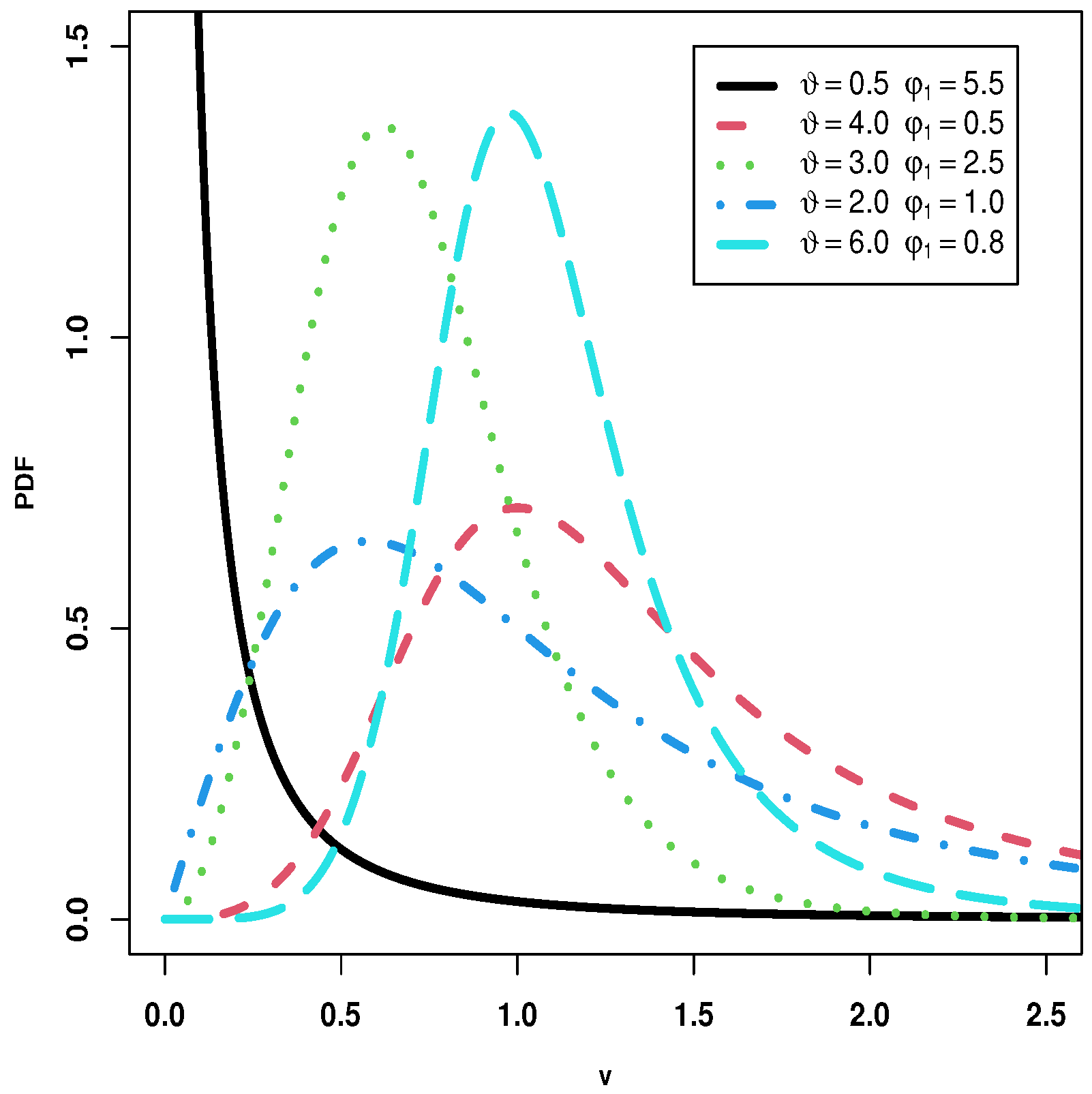The BXII distribution has recently been applied to a number of disciplines, including finance and economics (McDonald and Richards [34], hydrology (Mielke and Johnson [35]), medicine (Wingo [36]), mineralogy (Cook and Johnson [37]). The probability density function (PDF) and the survival (SF) of the BXII distribution are defined by:

$$h\left(v\right)=\vartheta {\phi }_1{v}^{\vartheta -1}{(1+v^{\vartheta })}^{-{\phi }_1-1}v\in {\mathbb{R}}^{+}$$

(1)

and

$$\overline{H}\left(v\right)={(1+v^{\vartheta })}^{-{\phi }_1}v\in {\mathbb{R}}^{+},$$

(2)

where $\vartheta ,{\phi }_1>0$ are the shape parameters. The BXII distribution’s inferences have been the subject of several studies (see, for example, [38,39,40,41,42,43,44]). Figure 1 shows the plots of PDF for the BXII distribution.

Figure 1. Plots of PDF for the BXII distribution.

On the other hand, the BIII distribution has a wide range of applications in statistical modeling fields, including forestry (Gove et al. [45]), meteorology (Mielke [46]), fracture roughness data (Nadarajah and Kotz [47], and life testing (Hassen et al. [48]). In studies of the distribution of income, wages, and wealth, the BIII distribution is also known as the Dagum distribution [30]. It is referred to as the inverse Burr distribution in the actuarial literature [49] and the Kappa distribution in the meteorological literature [46]. 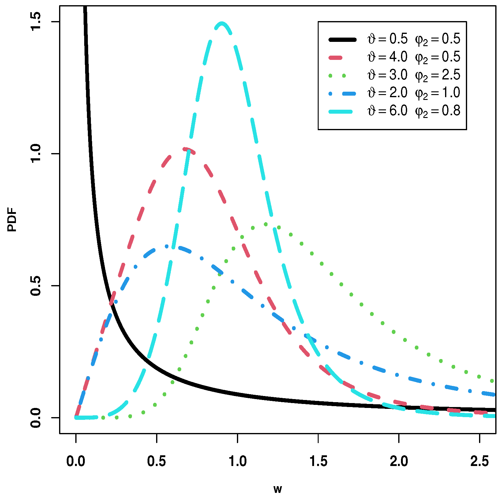For a random variable $w\in {\mathbb{R}}^{+}$, the PDF and SF of the BIII distribution, respectively, are given below:

$$g\left(w\right)=\vartheta {\phi }_2{w}^{-(\vartheta +1)}{(1+w^{-\vartheta })}^{-{\phi }_2-1},$$

(3)

and

$$\overline{G}\left(w\right)=1-{(1+w^{-\vartheta })}^{-{\phi }_2},$$

(4)

where $\vartheta ,{\phi }_2>0$, are the shape parameters. Several studies have looked at the implications of the BIII distribution (for instance, [50,51,52,53]). Figure 2 shows the plots of PDF for the BIII distribution.

Figure 2. Plots of PDF for the BIII distribution.

Let strength V∼ BXII $(\vartheta ,{\phi }_1)$ and stress W∼BIII $(\vartheta ,{\phi }_2)$ be independently distributed random variables with the common shape parameter $\vartheta$ and the different shape parameter $({\phi }_1,{\phi }_2).$ The SS reliability formula of $\delta =P\left[W<V\right]$ is computed as follows:

$$\begin{array}{c}\delta =\underset{0}{\overset{\infty }{\int }}h\left(v\right)H_W\left(v\right)dv=\underset{0}{\overset{\infty }{\int }}\vartheta {\phi }_1{v}^{\vartheta -1}{(1+v^{\vartheta })}^{-{\phi }_1-1}{(1+v^{-\vartheta })}^{-{\phi }_2}dv\hfill \\ ={\phi }_1\mathrm{B}\left({\phi }_2+1,{\phi }_1\right)=\left[\frac{\mathrm{\Gamma }({\phi }_1+1)\mathrm{\Gamma }({\phi }_2+1)}{\mathrm{\Gamma }({\phi }_1+{\phi }_2+1)}\right],\hfill \end{array}$$

(5)

where $\mathrm{\Gamma }(.)$ is the gamma function. The SS parameter $\delta$ depends on the shape parameters ${\phi }_1$ and ${\phi }_2$.

3. Maximum Likelihood Estimator of $\mathit{\delta }$

Let $(v_{1:m_1:n_1},\dots ,v_{m_1:m_1:n_1})=(v_1,\dots ,v_{m_1})$ be the TII-PC from BXII $(\vartheta ,{\phi }_1)$ with censoring scheme $R=(R_1,\dots ,R_{m_1})$ having PDF (1) and SF (2). Let $(w_{1:m_2:n_2},\dots ,w_{m_2:m_2:n_2})=(w_1,\dots ,v_{m_2})$ be the TII-PC from BIII $(\vartheta ,{\phi }_2)$ with censoring scheme $R^{\circ }=(R_1^{\circ },\dots ,R{m}_{{}_2}^{\circ })$ having PDF (3) and SF (4). The joint likelihood function is obtained as follows:

$$L=K_1{K}_2\prod _{i=1}^{m_1}{h}_V(v_i){\left[{\overline{H}}_V\left(v_i\right)\right]}^{R_i}\prod _{j=1}^{m_2}{g}_W\left(w_j\right){\left[{\overline{G}}_W\left(w_j\right)\right]}^{R_j^{\circ }},$$

(6)

where

$$K_1=n_1(n_1-1-R_1)(n_1-2-R_1-R_2)\times ...\times (n_1-m_1+1-R_1-...-R_{m_1}-1),$$

and

$$K_2=n_2(n_2-1-R_1^{\circ })(n_2-2-R_1^{\circ }-R_2^{\circ })\times ...\times (n_2-m_2+1-R_1^{\circ }-...-R_{m_2}^{\circ }-1).$$

Using (1), (2), (3), and (4) in (6) we have

$$L\propto {\left(\vartheta {\phi }_1\right)}^{m_1}{\left(\vartheta {\phi }_2\right)}^{m_2}\prod _{i=1}^{m_1}{v}_i^{\vartheta -1}{(1+v_i^{\vartheta })}^{-{\phi }_1-1}{\left[{(1+v_i^{\vartheta })}^{-{\phi }_1}\right]}^{R_i}\prod _{j=1}^{m_2}{w}_j^{-\left(\vartheta +1\right)}{(1+w_j^{-\vartheta })}^{-{\phi }_2-1}{\left[1-{(1+w_j^{-\vartheta })}^{-{\phi }_2}\right]}^{R_j^{\circ }}.$$

(7)

Now, the log-likelihood of (7) is:

$$\begin{array}{c}{\ell }^{*}\propto m_{1}ln\left(\vartheta {\phi }_1\right)+m_{2}ln\left(\vartheta {\phi }_2\right)+\vartheta \left[{\displaystyle \sum _{i=1}^{m_1}}ln\left(v_i\right)-{\displaystyle \sum _{j=1}^{m_2}}ln\left(w_j\right)\right]\hfill \\ -({\phi }_1+1){\displaystyle \sum _{i=1}^{m_1}}ln(1+\underset{i}{\overset{\vartheta }{v}})-{\displaystyle \sum _{i=1}^{m_1}}{R}_i{\phi }_{1}ln(1+\underset{i}{\overset{\vartheta }{v}})\hfill \\ -({\phi }_2+1){\displaystyle \sum _{j=1}^{m_2}}ln(1+\underset{j}{\overset{-\vartheta }{w}})+{\displaystyle \sum _{j=1}^{m_2}}\underset{j}{\overset{\circ }{R}}ln\left[1-{(1+\underset{j}{\overset{-\vartheta }{w}})}^{-{\phi }_2}\right].\hfill \end{array}$$

(8)

Differentiating (8) with regard to $\vartheta ,{\phi }_1$, and ${\phi }_2$ and then equalizing them to zero, we obtain

$$\begin{array}{c}\frac{\partial {\ell }^{*}}{\partial \vartheta }=\frac{m_1+m_2}{\widehat{\vartheta }}+\sum _{i=1}^{m_1}ln\left(v_i\right)-\sum _{j=1}^{m_2}ln\left(w_j\right)-({\widehat{\phi }}_1+1)\sum _{i=1}^{m_1}\frac{ln{v}_i}{(1+\underset{i}{\overset{-\widehat{\vartheta }}{v}})}-\sum _{i=1}^{m_1}\frac{R_i{\widehat{\phi }}_{1}ln{v}_i}{(1+\underset{i}{\overset{-\widehat{\vartheta }}{v}})}\hfill \\ +({\widehat{\phi }}_2+1)\sum _{j=1}^{m_2}\frac{ln{w}_j}{(1+\underset{j}{\overset{\widehat{\vartheta }}{w}})}-\sum _{j=1}^{m_2}\frac{\underset{j}{\overset{\circ }{R}}{\widehat{\phi }}_2{(1+\underset{j}{\overset{-\widehat{\vartheta }}{w}})}^{-{\widehat{\phi }}_2-1}\underset{j}{\overset{-\widehat{\vartheta }}{w}}ln{w}_j}{1-{(1+\underset{j}{\overset{-\vartheta }{w}})}^{-{\widehat{\phi }}_2}}=0,\hfill \end{array}$$

(9)

$$\frac{\partial {\ell }^{*}}{\partial {\phi }_1}=\frac{m_1}{{\widehat{\phi }}_1}-\sum _{i=1}^{m_1}ln(1+v_i^{\widehat{\vartheta }})-\sum _{i=1}^{m_1}{R}_{i}ln(1+v_i^{\widehat{\vartheta }})=0,$$

(10)

and

$$\frac{\partial {\ell }^{*}}{\partial {\phi }_2}=\frac{m_2}{{\widehat{\phi }}_2}-\sum _{j=1}^{m_2}ln(1+w_j^{-\widehat{\vartheta }})+\sum _{j=1}^{m_2}\frac{R_j^{\circ }ln(1+w_j^{-\widehat{\vartheta }})}{\left[{(1+w_j^{-\widehat{\vartheta }})}^{{\widehat{\phi }}_2}-1\right]}=0.$$

(11)

It is obvious that the normal Equations (9)–(11) lack explicit forms. The Newton–Raphson technique is used to obtain MLEs of $\vartheta ,{\phi }_1$, and ${\phi }_2$.

Furthermore, we assumed that $R_i,i=1,\dots ,m_1$, $R_j^{\circ },j=1,\dots ,m_2$ are independent random variables following binomial distributions. Hence,

$$P(R_1=r_1)=\left(\begin{array}{c}{n}_1-m_1\\ r_1\end{array}\right)P_1^{r_1}{\left(1-P_1\right)}^{n_1-m_1-r_1},$$

and

$$P\left(R_i=r_i\left|R_{i-1}=r_{i-1},\dots ,R_1=r_1\right.\right)=\left(\begin{array}{c}{n}_1-m_1-\sum _{s_1=1}^{i-1}{r}_{s_1}\\ r_i\end{array}\right)P_1^{r_i}{\left(1-P_1\right)}^{n_1-m_1-\sum _{s_1=1}^{i-1}{r}_{s_1}},$$

where $0⩽r_1⩽n_1-m_1,0⩽r_i⩽n_1-m_1-\sum _{s_1=1}^{i-1}{r}_{s_1},i=2,\dots ,m_1-1,R_{m_1}=n_1-m_1-\sum _{s_1=1}^{m_1-1}{r}_{s_1}$. Similarly,

$$P(R_1^{\circ }=r_1^{\circ })=\left(\begin{array}{c}{n}_2-m_2\\ r_1^{\circ }\end{array}\right)P_2^{r_{{}_1}^{\circ }}{\left(1-P_2\right)}^{n_2-m_2-r_1^{\circ }},$$

and

$$P\left(R_j^{\circ }=r_j^{\circ }\left|R_{j-1}^{\circ }=r_{j-1}^{\circ },\dots .,R_1^{\circ }=r_1^{\circ }\right.\right)=\left(\begin{array}{c}{n}_2-m_2-\sum _{s_2=1}^{j-1}{r}_{s_2}^{\circ }\\ r_j^{\circ }\end{array}\right)P_2^{r_j^{\circ }}{\left(1-P_2\right)}^{n_2-m_2-\sum _{s_2=1}^{j-1}{r}_{s_2}^{\circ }},$$

where $0⩽r_1^{\circ }⩽n_2-m_2,0⩽r_j^{\circ }⩽n_2-m_2-\sum _{s_2=1}^{j-1}{r}_{s_2}^{\circ },j=2,\dots ,m_2-1,R_{m_2}^{\circ }=n_2-m_2-\sum _{s_2=1}^{m_2-1}{r}_{s_2}^{\circ }$. The LF is, therefore, provided by

$$\begin{array}{c}{L}_1=L\times P(R_1=r_1,\dots ,R_{m_1}=r_{m_1})\times P(R_1^{\circ }=r_1^{\circ },\dots ,R_{m_2}^{\circ }=r_{m_2}^{\circ })\hfill \\ =L\times \frac{n_1-m_1}{\prod _{i=1}^{m_1-1}{r}_i!\left(n_1-m_1-\sum _{i=1}^{m_1-1}{r}_i\right)!}{P}_1^{\sum _{i=1}^{m_1-1}{r}_i}{\left(1-P_1\right)}^{(m_1-1)(n_1-m_1)-\sum _{i=1}^{m_1-1}(m_1-i)r_i}\hfill \\ \times \frac{n_2-m_2}{\prod _{j=1}^{m_2-1}{r}_j^{\circ }!\left(n_2-m_2-\sum _{j=1}^{m_2-1}{r}_j^{\circ }\right)!}{P}_2^{\sum _{j=1}^{m_2-1}{r}_j^{\circ }}{\left(1-P_2\right)}^{(m_2-1)(n_2-m_2)-\sum _{j=1}^{m_2-1}(m_2-j)r_j^{\circ }}.\hfill \end{array}$$

(12)

As observed, the joint PDF of $R_i{}^{,}s,i=1,\dots ,m_1$ and $R_j^{\circ ,}s,j=1,\dots ,m_2$ depend on $P_1$ and $P_2$. Hence, the MLEs of $P_1$ and $P_2$ are obtained by maximizing $L_1$ as below:

$${\widehat{P}}_1=\frac{\sum _{i=1}^{m_1-1}{r}_i}{(m_1-1)(n_1-m_1)-\sum _{i=1}^{m_1-1}(m_1-i-1)r_i},{\widehat{P}}_2=\frac{\sum _{j=1}^{m_2-1}{r}_j^{\circ }}{(m_2-1)(n_2-m_2)-\sum _{j=1}^{m_2-1}(m_2-j-1)r_j^{\circ }}.$$

Finally, the MLE of $\delta$ is obtained by inserting ${\widehat{\phi }}_1$ and ${\widehat{\phi }}_2$ in Equation (5) as follows:

$$\widehat{\delta }=\left[\frac{\Gamma ({\widehat{\phi }}_1+1)\Gamma ({\widehat{\phi }}_2+1)}{\Gamma ({\widehat{\phi }}_1+{\widehat{\phi }}_2+1)}\right].$$

4. Bayesian Estimation

This section provides the Bayesian estimator of $\delta$ based on TII-PC with binomial removals, under the SEF and LNx loss functions, using INF and N-INF priors. We assume that the prior PDFs of $\vartheta ,{\phi }_1$, and ${\phi }_2$ are given, respectively, by:

$${\pi }_k\left({\phi }_k\right)=\frac{b_k^{a_k}}{\Gamma \left(a_k\right)}{\phi }_k^{a_k-1}{e}^{-b_k{\phi }_k},a_k,b_k,{\phi }_k>0,k=1,2,$$

(13)

and

$${\pi }_3\left(\vartheta \right)=\frac{b_3^{a_3}}{\Gamma \left(a_3\right)}{\vartheta }^{a_3-1}{e}^{-b_3\vartheta },a_3,b_3,\vartheta >0.$$

(14)

The joint posterior PDF of $\vartheta ,{\phi }_1$, and ${\phi }_2$ is given by

$${\pi }^{•}({\phi }_1,{\phi }_2,\vartheta )\propto L_1{\phi }_1^{a_1-1}{\phi }_2^{a_2-1}{\vartheta }^{a_3-1}{b}_1^{a_1}{b}_2^{a_2}{b}_3^{a_3}{e}^{-(b_1{\phi }_1+b_2{\phi }_2+b_3\vartheta )}.$$

(15)

Since $0<P_j<1,j=1,2$, we consider the following prior PDFs for $P_j,j=1,2$

$${\pi }_k\left(P_j\right)=\frac{1}{\mathrm{B}(c_j,d_j)}{P}_j^{c_j-1}{(1-P_j)}^{d_j-1},j=1,2,k=4,5,$$

(16)

where $B(.,.)$ is the beta function. The joint posterior PDF of ${\phi }_1,{\phi }_2,\vartheta ,P_1$, and $P_2$ is given by:

$${\pi }^{••}({\phi }_1,{\phi }_2,\vartheta ,P_1,P_2)\propto L_1{\phi }_1^{a_1-1}{\phi }_2^{a_2-1}{\vartheta }^{a_3-1}{b}_1^{a_1}{b}_2^{a_2}{b}_3^{a_3}{e}^{-(b_1{\phi }_1+b_2{\phi }_2+b_3\vartheta )}{\pi }_4\left(P_1\right){\pi }_5\left(P_2\right).$$

(17)

Using (12), we have

$${\pi }^{••}({\phi }_1,{\phi }_2,\vartheta ,P_1,P_2)=D^{*}{\pi }^{•}({\phi }_1,{\phi }_2,\vartheta ),$$

where

$$\begin{array}{c}{D}^{*}=\frac{P_1^{{\displaystyle \sum }_{i=1}^{m_1-1}{r}_i+c_1-1}{\left(1-P_1\right)}^{(m_1-1)(n_1-m_1)-{\displaystyle \sum }_{i=1}^{m_1-1}(m_1-i)r_i+d_1-1}}{\mathrm{B}\left({\displaystyle \sum }_{i=1}^{m_1-1}{r}_i+c_1,(m_1-1)(n_1-m_1)-{\displaystyle \sum }_{i=1}^{m_1-1}(m_1-i)r_i+d_1\right)}\hfill \\ \times \frac{P_2^{{\displaystyle \sum }_{j=1}^{m_2-1}{r}_j^{\circ }+c_2-1}{\left(1-P_2\right)}^{(m_2-1)(n_2-m_2)-{\displaystyle \sum }_{j=1}^{m_2-1}(m_2-j)r_j^{\circ }+d_2-1}}{\mathrm{B}\left({\displaystyle \sum }_{j=1}^{m_2-1}{r}_j^{\circ }+c_2,(m_2-1)(n_2-m_2)-\sum _{j=1}^{m_2-1}(m_2-j)r_j^{\circ }+d_2\right)}.\hfill \end{array}$$

The conditional posteriors are given as:

1.

For ${\phi }_1$:

$$\pi \left({\phi }_1\right|{\phi }_2,\vartheta ,P_1,P_2)\propto {\phi }_1^{a_1-1}{e}^{-b_1{\phi }_1}\prod _{i=1}^{m_1}{(1+v_i^{\vartheta })}^{-{\phi }_1{R}_i}\prod _{j=1}^{m_2}{(1+w_j^{-\vartheta })}^{-{\phi }_1{R}_j^{\circ }}$$

2.

For ${\phi }_2$:

$$\pi \left({\phi }_2\right|{\phi }_1,\vartheta ,P_1,P_2)\propto {\phi }_2^{a_2-1}{e}^{-b_2{\phi }_2}\prod _{i=1}^{m_1}{(1+v_i^{\vartheta })}^{-{\phi }_2{R}_i}\prod _{j=1}^{m_2}{(1-{(1+w_j^{-\vartheta })}^{-{\phi }_2})}^{R_j^{\circ }}$$

3.

For $\vartheta$:

$$\pi \left(\vartheta \right|{\phi }_1,{\phi }_2,P_1,P_2)\propto {\vartheta }^{a_3-1}{e}^{-b_3\vartheta }\prod _{i=1}^{m_1}{v}_i^{\vartheta -1}{(1+v_i^{\vartheta })}^{-{\phi }_1}\prod _{j=1}^{m_2}{w}_j^{-(\vartheta +1)}{(1+w_j^{-\vartheta })}^{-{\phi }_2}$$

4.

For $P_1$:

$$\pi \left(P_1\right|{\phi }_1,{\phi }_2,\vartheta ,P_2)\propto P_1^{{\sum }_{i=1}^{m_1-1}{r}_i+c_1-1}{(1-P_1)}^{({\sum }_{i=1}^{m_1-1}(m_1-i)r_i+d_1-1)}$$

5.

For $P_2$:

$$\pi \left(P_2\right|{\phi }_1,{\phi }_2,\vartheta ,P_1)\propto P_2^{{\sum }_{j=1}^{m_2-1}{r}_j^{\circ }+c_2-1}{(1-P_2)}^{({\sum }_{j=1}^{m_2-1}(m_2-j)r_j^{\circ }+d_2-1)}$$

From the above conditional posteriors, which appear complex, we will not be able to obtain a distribution to generate samples from these relationships. Therefore, we will use a numerical method to solve the integration of the original posterior distribution, in Equation (17), such as the Markov Chain Monte Carlo (MCMC) method.

The Bayesian estimator of $\delta$ is defined as ${\tilde{\delta }}_{SEF}$ and ${\tilde{\delta }}_{LNx}$, respectively, where it minimizes the SEF $L_{SEF}\left(\delta ,{\tilde{\delta }}_{SEF}\right)$, loss function, and LNx loss function, $L_{LNx}\left(\delta ,{\tilde{\delta }}_{LNx}\right).$

$$L_{SEF}\left(\delta ,{\tilde{\delta }}_{SEF}\right)={\left(\delta -{\tilde{\delta }}_{SEF}\right)}^2,$$

(18)

$$L_{LNx}\left(\delta ,{\tilde{\delta }}_{LNx}\right)=e^{\alpha (\delta -{\tilde{\delta }}_{LNx})}-\alpha \left(\delta -{\tilde{\delta }}_{LNx}\right)-1,$$

(19)

and

$$\begin{array}{cc}\hfill {\tilde{\delta }}_{SEF}& =E\left(\delta \right)\hfill \\ \hfill {\tilde{\delta }}_{LNx}& =\frac{-1}{\alpha }ln\left[E\left(e^{-\alpha \delta }\right)\right],\hfill \end{array}$$

(20)

where $\alpha$ is an LNx scale parameter (for further information, see [54]). It should be clear that it is impossible to calculate Equation (20) analytically. Approximating these equations can be achieved with the Metropolis–Hastings (MH) method and the MCMC technique.

4.1. MH Algorithm

The MH method (Algorithm 1) uses the stages listed below to draw a sample from the posterior density provided by Equation (20)

Algorithm 1:
Step 1.	Initialize $\xi$ with $\xi =\left({\vartheta }^{\left(0\right)},{\varphi }_1^{\left(0\right)},{\varphi }_2^{\left(0\right)}\right)=\left(\widehat{\vartheta },{\widehat{\varphi }}_1,{\widehat{\varphi }}_2\right)$, where $P_1$ and $P_2$ are fixed.
Step 2.	For $i=1,2,\dots ,M$, perform the following steps:
2.1:	Set $\xi ={\xi }^{(i-1)}$.
2.2:	Generate a new candidate parameter value ${\xi }^{{}^{\prime }}$ using a normal distribution with mean vector ${\xi }^{(i-1)}$ and a small vector of standard deviations.
2.3:	Compute $\beta =\frac{{\pi }^{••}\left({\xi }^{{}^{\prime }}\right)}{{\pi }^{••}({\xi }^{)}}$, where ${\pi }^{••}(·)$ is the posterior density in Equation (20).
2.4:	Generate a sample u from the uniform $U(0,1)$ distribution.
2.5:	Accept or reject the new candidate ${\xi }^{{}^{\prime }}$ $$\left\{\begin{array}{cc}\mathrm{If}u\le \beta \hfill & \mathrm{set}{\xi }^{\left(i\right)}={\xi }^{{}^{\prime }}\hfill \\ \mathrm{elsewhere}\hfill & \mathrm{set}{\xi }^{\left(i\right)}=\xi \end{array}\right.$$

Therefore, MCMC samples of $(\vartheta ,{\varphi }_1,{\varphi }_2)$ are obtained as:

$${\xi }^{\left(i\right)}=\left({\vartheta }^{\left(i\right)},{\varphi }_1^{\left(i\right)},{\varphi }_2^{\left(i\right)}\right),i=1,2,\dots ,M.$$

Hence, $\delta$ can be computed by substituting ${\xi }^{\left(i\right)}$ in Equation (5). Eventually, a portion of the initial samples can be removed (burn-in), and the remaining samples can be used to calculate Bayesian estimates (BEs) using random samples of size M drawn from the posterior density. The BEs of a parametric function $\delta$ under SEF and LNx are given by

$${\widehat{\delta }}_{SE}=\frac{1}{M-l_B}\sum _{i=l_B}^M{\delta }^{\left(i\right)},$$

(21)

and

$${\widehat{\delta }}_{LNx}=\frac{-1}{\alpha }ln\left[\frac{1}{M-l_B}\sum _{i=l_B}^M{\mathrm{e}}^{-\alpha {\delta }^{\left(i\right)}}\right],$$

(22)

where $l_B$ represents the number of burn-in samples. Substituting ${\delta }^{\left(i\right)}$ with ${\xi }^{\left(i\right)}$ in the above equations, we can obtain BEs of $\delta$ with respect to SEF and LNx loss functions.

4.2. Elicitation of Hyper-Parameters

The determination of hyper-parameters relies on informative priors, derived from the MLEs for BXII$(\vartheta ,{\varphi }_1)$. This is achieved by aligning the mean and variance of $({\widehat{\vartheta }}^j,{\widehat{\varphi }}_1^j)$ with the corresponding parameters of gamma priors. Here, $j=1,2,\dots ,f$, and f denotes the number of available samples from the BXII$(\vartheta ,{\varphi }_1)$ distribution (Dey et al. [55]). Equating the moments of $({\widehat{\vartheta }}^j,{\widehat{\varphi }}_1^j)$ with the moments of the gamma priors yields the following equations:

$$\begin{array}{cc}\hfill \frac{1}{f}\sum _{j=1}^f{\widehat{\vartheta }}^j& =\frac{a_1}{b_1},\frac{1}{f-1}\sum _{j=1}^f{\left({\widehat{\vartheta }}^j-\frac{1}{f}\sum _{j=1}^f{\widehat{\vartheta }}^j\right)}^2=\frac{a_1}{b_1^2},\hfill \\ \hfill \frac{1}{f}\sum _{j=1}^f{\widehat{\varphi }}_1^j& =\frac{a_2}{b_2}\mathrm{and}\frac{1}{f-1}\sum _{j=1}^f{\left({\widehat{\varphi }}_1^j-\frac{1}{f}\sum _{j=1}^f{\widehat{\varphi }}_1^j\right)}^2=\frac{a_2}{b_2^2}.\hfill \end{array}$$

By solving the mentioned pair of equations, we can express the estimated hyper-parameters as follows:

$$\begin{array}{cc}\hfill a_1& =\frac{{\left(\frac{1}{f}{\sum }_{j=1}^f{\widehat{\vartheta }}^j\right)}^2}{\frac{1}{f-1}{\sum }_{j=1}^f({\widehat{\vartheta }}^j-\frac{1}{f}{\sum }_{j=1}^f{\widehat{\vartheta }}^j{)}^2},b_1=\frac{\frac{1}{f}{\sum }_{j=1}^f{\widehat{\vartheta }}^j}{\frac{1}{f-1}{\sum }_{j=1}^f{\left({\widehat{\vartheta }}^j-\frac{1}{f}{\sum }_{j=1}^f{\widehat{\vartheta }}^j\right)}^2}\hfill \\ \hfill a_2& =\frac{(\frac{1}{f}{\sum }_{j=1}^k{\widehat{\varphi }}_1^j{)}^2}{\frac{1}{k-1}{\sum }_{j=1}^f({\widehat{\varphi }}_1^j-\frac{1}{f}{\sum }_{j=1}^f{\widehat{\varphi }}_1^j{)}^2},b_2=\frac{\frac{1}{f}{\sum }_{j=1}^f{\widehat{\varphi }}_1^j}{\frac{1}{f-1}{\sum }_{j=1}^f{\left({\widehat{\varphi }}_1^j-\frac{1}{f}{\sum }_{j=1}^f{{\widehat{\varphi }}_1}^j\right)}^2}.\hfill \end{array}$$

(23)

We will apply the identical technique to calculate the hyper-parameters $(a_3,b_3,a_4,b_4)$ for the BIII($\vartheta ,{\varphi }_2$) case. Here, $\vartheta$ remains consistent across two assumed distributions, implying that its hyper-parameters assume identical values, specifically $a_1=a_3$ and $b_1=b_3$.

5. Numerical Outcomes

In this section, we investigate the application of Monte Carlo simulation to the proposed estimates of the SS reliability $\delta$ within the context of TII-PC, incorporating binomial removal. The primary objective of this simulation study is to scrutinize the properties and effectiveness of derived estimates through both the ML and Bayesian methods. It is worth noting that the numerical calculations were executed using the R programming language, alongside various auxiliary software packages, to facilitate equation solving and result extraction. The following arguments are assumed for the simulation process:

1.

We assume a total of 1000 replications for our simulations.

2.

We assume the parameters for BXII($\vartheta ,{\phi }_1$) and BIII($\vartheta ,{\phi }_2$) are configured as follows: ${\phi }_1$ takes values of 0.5 and 1.5, and ${\phi }_2$ takes values of 0.75 and 1.75. Here, $\vartheta$ remains constant across both distributions, set at 1.5. Generating all potential parameter combinations will yield four distinct cases.

3.

We suggest a sample size of $n=n_1=n_2$ with two values: 40 and 60. Furthermore, the number of stages $m=m_1=m_2$, varies depending on the chosen n value. Specifically, when $n=40$, we configure m to be either 20 or 30. On the other hand, for $n=60$, we explore options with $m=25$ and 40 stages.

4.

In simulating the removal of units from the life test, we model it following a binomial distribution with probability $P=P_1=P_2$. We explore various values for the probability $P=$ 0.05, 0.20, 0.50, and 0.8. Concerning the random unit removal patterns in the TII-PC, we assume two primary patterns based on n, m, and the removal probability P, falling into two distinct cases:

Scheme 1 (Sch-1):

$R_1$ follows a binomial distribution with parameters $(n-m-1,P)$, and subsequent stages $R_j$ follow a binomial distribution with parameters $(n-{\sum }_{j=2}^{m-1}{R}_j,P)$, where $j=2,\dots ,m-1$. In this scheme, $R_m$ is set to zero.

Scheme 2 (Sch-2):

Here, $R_m$ follows a binomial distribution with parameters $(n-m-1,P)$ and preceding stages $R_{m-j}$ follow a binomial distribution with parameters $(n-{\sum }_{j=m-1}^m{R}_j,P)$. In this scheme, $R_1$ is set to zero.

Notably, Sch-1 involves a decreasing number of removals at each stage of censoring, while Sch-2 exhibits an increasing trend.

Steps of the Monte Carlo Simulation

Step 1:

For Sch-1, generate two random vectors of removed items, namely R and $R^{\circ }$, given ($n_1,m_1$$,P_1$) and where ($n_2,m_2$$,P_2$), $n=n_1=n_2,m=m_1=m_2$ and $P=P_1=P_2$.

Step 2:

Generate a random data set V of size $n=n_1$ from $\mathrm{BXII}(\vartheta ,{\phi }_1)$ using the algorithm proposed by [56] and the provided R.

Step 3:

Similarly, generate a random data set W of size $n=n_2$ from the $\mathrm{BIII}(\vartheta ,{\phi }_2)$ given $R^{\circ }$.

Step 4:

Obtain MLE for the parameters $\vartheta$, ${\phi }_1$, and ${\phi }_2$, and subsequently compute the estimate for $\delta$ by plugging these MLEs of ($\vartheta$, ${\phi }_1$, and ${\phi }_2$) into Equation (5).

Step 5:

Compute the BE using the MH algorithm as follows:

1.

Consider two scenarios for prior distributions. In the first scenario, an INF prior is employed, where hyper-parameter values are computed using the technique outlined in Section 4.2 and Equations (23).

2.

Consider the second scenario, which involves the N-INF prior, where all hyper-parameter values are set to zero.

3.

For the given hyper-parameters of prior distributions, generate 10,000 samples of $\delta$ from the posterior density using MCMC and the MH algorithm.

4.

Discard the initial 2000 samples as burn-in from the overall set of 8000 samples generated from the posterior density.

5.

Calculate BEs of $\delta$ using two loss functions: SEF and LNx (with $\alpha =-1.5$ for $LN{x}_1$ and $\alpha =1.5$ for $LN{x}_2)$ using, respectively, (21) and (22).

Step 6:

Repeat Steps 2 to 5 a total of 1000 times and save all the estimates.

Step 7:

Calculate statistical metrics for point estimates: the average (A1) estimate and the root mean square error (A2) estimate. These calculations can be performed using the following formulas:

$$A1\left(\delta \right)=\frac{1}{1000}\sum _{l=1}^{1000}{\widehat{\delta }}_l,\mathrm{and}A2\left(\delta \right)=\sqrt{\frac{1}{1000}\sum _{l=1}^{1000}{({\widehat{\delta }}_l-\delta )}^2}.$$

In this context, $\delta$ signifies the actual value of the SS with the provided parameters, whereas $\widehat{\delta }$ indicates the estimated value of the SS.

Step 8:

Repeat Steps 1 to 7 for the second scheme of removing items (Sch-2).

To provide point estimates of $\delta$, we present the results of A1 and A2 estimates for various values of P and two proposed TII-PC schemes. Table 1 and Table 2 correspond to cases, where ${\phi }_1=0.5$ and ${\phi }_2$ take values of 0.75 and 1.75, respectively. Additionally, Table 3 and Table 4 correspond to cases where ${\phi }_1=1.5$ and ${\phi }_2$ take values of 0.75 and 1.75, respectively. The first row includes the A1 of $\delta$ and the second row includes the A2 of $\delta$.

Table 1. Measures of the MLEs and BEs for ${\phi }_1=0.5$ and ${\phi }_2=0.75$ under different values of P, m, and n.

( $n,m$)	P	Sch.		MLE	BE: INF			BE: N-INF
					SEF	${\mathit{LNx}}_1$	${\mathit{LNx}}_2$	SEF	${\mathit{LNx}}_1$	${\mathit{LNx}}_2$
(40, 20)	0.05	Sch-1	A1	0.8536	0.7973	0.7968	0.7979	0.8674	0.8662	0.8685
			A2	0.1390	0.0792	0.0786	0.0797	0.1519	0.1508	0.1530
		Sch-2	A1	0.8234	0.7860	0.7854	0.7866	0.8398	0.8381	0.8414
			A2	0.1117	0.0681	0.0675	0.0687	0.1263	0.1249	0.1278
	0.20	Sch-1	A1	0.8084	0.7822	0.7815	0.7828	0.8260	0.8241	0.8278
			A2	0.0994	0.0644	0.0638	0.0650	0.1142	0.1127	0.1158
		Sch-2	A1	0.8524	0.7981	0.7976	0.7987	0.8658	0.8646	0.8669
			A2	0.1378	0.0800	0.0795	0.0806	0.1503	0.1492	0.1513
	0.40	Sch-1	A1	0.7537	0.7676	0.7669	0.7683	0.7765	0.7739	0.7790
			A2	0.0590	0.0503	0.0496	0.0509	0.0726	0.0709	0.0743
		Sch-2	A1	0.8591	0.8010	0.8005	0.8016	0.8716	0.8706	0.8727
			A2	0.1441	0.0829	0.0824	0.0834	0.1558	0.1548	0.1568
	0.80	Sch-1	A1	0.7405	0.7645	0.7638	0.7652	0.7646	0.7617	0.7674
			A2	0.0562	0.0474	0.0467	0.0480	0.0665	0.0650	0.0680
		Sch-2	A1	0.8597	0.8012	0.8007	0.8017	0.8721	0.8711	0.8731
			A2	0.1447	0.0831	0.0825	0.0836	0.1563	0.1554	0.1573
(40,30)	0.05	Sch-1	A1	0.7781	0.7742	0.7736	0.7747	0.7918	0.7901	0.7935
			A2	0.0722	0.0568	0.0563	0.0574	0.0830	0.0817	0.0844
		Sch-2	A1	0.7566	0.7679	0.7673	0.7685	0.7715	0.7695	0.7734
			A2	0.0573	0.0509	0.0503	0.0514	0.0669	0.0656	0.0682
	0.20	Sch-1	A1	0.7432	0.7640	0.7634	0.7647	0.7588	0.7567	0.7609
			A2	0.0493	0.0471	0.0465	0.0477	0.0574	0.0562	0.0586
		Sch-2	A1	0.8133	0.7862	0.7857	0.7868	0.8242	0.8228	0.8256
			A2	0.1007	0.0684	0.0678	0.0689	0.1106	0.1094	0.1118
	0.40	Sch-1	A1	0.7327	0.7607	0.7601	0.7614	0.7491	0.7468	0.7513
			A2	0.0481	0.0441	0.0435	0.0447	0.0535	0.0526	0.0544
		Sch-2	A1	0.8321	0.7921	0.7916	0.7926	0.8425	0.8413	0.8437
			A2	0.1188	0.0742	0.0737	0.0748	0.1284	0.1273	0.1294
	0.80	Sch-1	A1	0.7259	0.7588	0.7582	0.7594	0.7426	0.7402	0.7449
			A2	0.0471	0.0422	0.0416	0.0428	0.0505	0.0498	0.0513
		Sch-2	A1	0.8408	0.7948	0.7943	0.7953	0.8507	0.8496	0.8518
			A2	0.1273	0.0769	0.0764	0.0774	0.1365	0.1355	0.1375
(60, 25)	0.05	Sch-1	A1	0.8526	0.8019	0.8014	0.8024	0.8633	0.8624	0.8642
			A2	0.1371	0.0839	0.0834	0.0843	0.1473	0.1465	0.1481
		Sch-2	A1	0.8379	0.7946	0.7940	0.7951	0.8499	0.8488	0.8509
			A2	0.1232	0.0766	0.0761	0.0771	0.1344	0.1334	0.1354
	0.20	Sch-1	A1	0.7781	0.7726	0.7719	0.7732	0.7949	0.7931	0.7966
			A2	0.0694	0.0550	0.0544	0.0556	0.0833	0.0818	0.0847
		Sch-2	A1	0.8571	0.8051	0.8046	0.8056	0.8672	0.8663	0.8680
			A2	0.1410	0.0871	0.0866	0.0875	0.1507	0.1499	0.1515
	0.40	Sch-1	A1	0.7476	0.7626	0.7619	0.7632	0.7665	0.7643	0.7686
			A2	0.0508	0.0456	0.0450	0.0462	0.0619	0.0606	0.0633
		Sch-2	A1	0.8615	0.8078	0.8073	0.8083	0.8713	0.8705	0.8720
			A2	0.1451	0.0897	0.0892	0.0901	0.1546	0.1539	0.1553
	0.80	Sch-1	A1	0.7389	0.7611	0.7605	0.7618	0.7589	0.7565	0.7613
			A2	0.0510	0.0444	0.0438	0.0451	0.0597	0.0585	0.0610
		Sch-2	A1	0.8595	0.8070	0.8066	0.8075	0.8696	0.8688	0.8703
			A2	0.1434	0.0890	0.0885	0.0894	0.1531	0.1523	0.1538
(60, 40)	0.05	Sch-1	A1	0.7912	0.7787	0.7781	0.7792	0.8009	0.7997	0.8020
			A2	0.0793	0.0613	0.0608	0.0618	0.0879	0.0869	0.0889
		Sch-2	A1	0.8351	0.7969	0.7965	0.7974	0.8427	0.8418	0.8435
			A2	0.1195	0.0790	0.0785	0.0794	0.1268	0.1260	0.1276
	0.20	Sch-1	A1	0.7439	0.7610	0.7604	0.7615	0.7560	0.7544	0.7575
			A2	0.0431	0.0442	0.0436	0.0447	0.0504	0.0494	0.0514
		Sch-2	A1	0.8435	0.8015	0.8010	0.8020	0.8507	0.8500	0.8515
			A2	0.1279	0.0836	0.0831	0.0840	0.1348	0.1341	0.1355
	0.40	Sch-1	A1	0.7350	0.7574	0.7568	0.7579	0.7475	0.7458	0.7491
			A2	0.0426	0.0410	0.0405	0.0415	0.0478	0.0470	0.0486
		Sch-2	A1	0.8505	0.8024	0.8019	0.8028	0.8572	0.8564	0.8579
			A2	0.1344	0.0843	0.0839	0.0847	0.1409	0.1402	0.1416
	0.80	Sch-1	A1	0.7307	0.7563	0.7557	0.7569	0.7430	0.7412	0.7447
			A2	0.0423	0.0400	0.0395	0.0406	0.0462	0.0455	0.0469
		Sch-2	A1	0.8520	0.8029	0.8025	0.8034	0.8591	0.8584	0.8598
			A2	0.1361	0.0849	0.0845	0.0853	0.1429	0.1423	0.1436

Table 2. Measures of the MLEs and BEs for ${\phi }_1=0.5$ and ${\phi }_2=1.75$ under different values of P, m, and n.

( $\mathit{n},\mathit{m}$)	P	Sch.		MLE	BE: INF			BE: N-INF
					SEF	${\mathit{LNx}}_1$	${\mathit{LNx}}_2$	SEF	${\mathit{LNx}}_1$	${\mathit{LNx}}_2$
(40, 20)	0.05	Sch-1	A1	0.7719	0.6699	0.6688	0.6709	0.7928	0.7909	0.7946
			A2	0.2170	0.1118	0.1107	0.1128	0.2372	0.2355	0.2390
		Sch-2	A1	0.7309	0.6475	0.6464	0.6486	0.7534	0.7510	0.7558
			A2	0.1763	0.0897	0.0886	0.0908	0.1979	0.1956	0.2002
	0.20	Sch-1	A1	0.6856	0.6289	0.6278	0.6301	0.7114	0.7085	0.7143
			A2	0.1339	0.0717	0.0706	0.0728	0.1584	0.1558	0.1610
		Sch-2	A1	0.7883	0.6768	0.6758	0.6778	0.8060	0.8043	0.8076
			A2	0.2335	0.1190	0.1180	0.1200	0.2506	0.2490	0.2521
	0.40	Sch-1	A1	0.6278	0.6062	0.6049	0.6074	0.6581	0.6546	0.6615
			A2	0.0872	0.0500	0.0488	0.0511	0.1111	0.1084	0.1139
		Sch-2	A1	0.8112	0.6871	0.6862	0.6881	0.8285	0.8271	0.8299
			A2	0.2554	0.1290	0.1281	0.1300	0.2722	0.2709	0.2735
	0.80	Sch-1	A1	0.6126	0.6011	0.5999	0.6024	0.6455	0.6418	0.6492
			A2	0.0711	0.0451	0.0440	0.0463	0.0977	0.0947	0.1008
		Sch-2	A1	0.8134	0.6894	0.6885	0.6904	0.8311	0.8298	0.8324
			A2	0.2575	0.1312	0.1303	0.1322	0.2747	0.2735	0.2760
(40, 30)	0.05	Sch-1	A1	0.6698	0.6310	0.6300	0.6320	0.6873	0.6850	0.6896
			A2	0.1219	0.0752	0.0743	0.0762	0.1378	0.1358	0.1398
		Sch-2	A1	0.6951	0.6411	0.6401	0.6421	0.7118	0.7096	0.7139
			A2	0.1435	0.0842	0.0833	0.0852	0.1587	0.1567	0.1606
	0.20	Sch-1	A1	0.5965	0.5981	0.5969	0.5992	0.6170	0.6142	0.6197
			A2	0.0593	0.0433	0.0423	0.0443	0.0731	0.0712	0.0751
		Sch-2	A1	0.7221	0.6527	0.6517	0.6536	0.7375	0.7355	0.7394
			A2	0.1684	0.0950	0.0940	0.0959	0.1834	0.1815	0.1852
	0.40	Sch-1	A1	0.5851	0.5935	0.5924	0.5945	0.6070	0.6043	0.6097
			A2	0.0561	0.0406	0.0397	0.0415	0.0690	0.0674	0.0707
		Sch-2	A1	0.7352	0.6602	0.6592	0.6612	0.7499	0.7480	0.7518
			A2	0.1813	0.1026	0.1016	0.1035	0.1953	0.1935	0.1971
	0.80	Sch-1	A1	0.5791	0.5897	0.5886	0.5908	0.6016	0.5987	0.6045
			A2	0.0641	0.0396	0.0387	0.0404	0.0741	0.0728	0.0755
		Sch-2	A1	0.7318	0.6586	0.6577	0.6596	0.7477	0.7458	0.7496
			A2	0.1781	0.1011	0.1002	0.1021	0.1932	0.1914	0.1949
(60, 25)	0.05	Sch-1	A1	0.8097	0.6888	0.6880	0.6896	0.8239	0.8228	0.8251
			A2	0.2527	0.1309	0.1301	0.1317	0.2667	0.2656	0.2678
		Sch-2	A1	0.7468	0.6534	0.6525	0.6544	0.7643	0.7626	0.7659
			A2	0.1913	0.0959	0.0950	0.0968	0.2087	0.2071	0.2103
	0.20	Sch-1	A1	0.6883	0.6258	0.6248	0.6268	0.7090	0.7067	0.7112
			A2	0.1356	0.0690	0.0680	0.0700	0.1549	0.1528	0.1570
		Sch-2	A1	0.8153	0.6941	0.6933	0.6950	0.8276	0.8265	0.8286
			A2	0.2583	0.1359	0.1351	0.1367	0.2706	0.2696	0.2716
	0.40	Sch-1	A1	0.6538	0.6113	0.6103	0.6124	0.6764	0.6739	0.6788
			A2	0.1026	0.0548	0.0538	0.0559	0.1241	0.1219	0.1264
		Sch-2	A1	0.8264	0.6974	0.6966	0.6982	0.8394	0.8385	0.8404
			A2	0.2696	0.1396	0.1388	0.1404	0.2825	0.2816	0.2833
	0.80	Sch-1	A1	0.6219	0.6010	0.5999	0.6021	0.6456	0.6426	0.6485
			A2	0.0775	0.0456	0.0446	0.0466	0.0968	0.0944	0.0993
		Sch-2	A1	0.8288	0.7015	0.7007	0.7023	0.8408	0.8399	0.8417
			A2	0.2718	0.1434	0.1426	0.1441	0.2839	0.2830	0.2847
(60, 40)	0.05	Sch-1	A1	0.6954	0.6402	0.6393	0.6411	0.7084	0.7069	0.7100
			A2	0.1409	0.0833	0.0825	0.0842	0.1533	0.1519	0.1548
		Sch-2	A1	0.7305	0.6574	0.6566	0.6582	0.7418	0.7404	0.7433
			A2	0.1742	0.0997	0.0989	0.1005	0.1853	0.1839	0.1867
	0.20	Sch-1	A1	0.6146	0.6016	0.6006	0.6025	0.6321	0.6301	0.6340
			A2	0.0691	0.0467	0.0459	0.0475	0.0854	0.0838	0.0869
		Sch-2	A1	0.7576	0.6708	0.6700	0.6716	0.7681	0.7669	0.7694
			A2	0.2008	0.1128	0.1120	0.1136	0.2112	0.2100	0.2124
	0.40	Sch-1	A1	0.5869	0.5889	0.5879	0.5898	0.6005	0.5985	0.6025
			A2	0.0478	0.0352	0.0344	0.0360	0.0578	0.0565	0.0591
		Sch-2	A1	0.7688	0.6765	0.6757	0.6772	0.7778	0.7767	0.7790
			A2	0.2121	0.1186	0.1178	0.1193	0.2213	0.2202	0.2224
	0.80	Sch-1	A1	0.5774	0.5861	0.5851	0.5871	0.5924	0.5901	0.5946
			A2	0.0460	0.0343	0.0335	0.0350	0.0541	0.0528	0.0553
		Sch-2	A1	0.7753	0.6805	0.6797	0.6812	0.7852	0.7841	0.7863
			A2	0.2184	0.1225	0.1217	0.1232	0.2283	0.2272	0.2294

Table 3. Measures of the MLEs and BEs for ${\phi }_1=1.5$ and ${\phi }_2=0.75$ under different values of P, m, and n.

( $\mathit{n},\mathit{m}$)	P	Sch.		MLE	BE: INF			BE: N-INF
					SEF	${\mathit{LNx}}_1$	${\mathit{LNx}}_2$	SEF	${\mathit{LNx}}_1$	${\mathit{LNx}}_2$
(40, 20)	0.05	Sch-1	A1	0.6344	0.5444	0.5432	0.5456	0.6614	0.6581	0.6647
			A2	0.1619	0.0671	0.0659	0.0682	0.1876	0.1845	0.1907
		Sch-2	A1	0.6133	0.5362	0.5349	0.5374	0.6426	0.6390	0.6461
			A2	0.1428	0.0594	0.0583	0.0606	0.1699	0.1666	0.1732
	0.20	Sch-1	A1	0.5727	0.5211	0.5198	0.5223	0.6050	0.6009	0.6090
			A2	0.1064	0.0449	0.0438	0.0461	0.1348	0.1312	0.1384
		Sch-2	A1	0.6432	0.5509	0.5497	0.5520	0.6697	0.6666	0.6728
			A2	0.1702	0.0734	0.0723	0.0746	0.1955	0.1925	0.1984
	0.40	Sch-1	A1	0.5292	0.5075	0.5062	0.5088	0.5647	0.5601	0.5693
			A2	0.0758	0.0332	0.0322	0.0343	0.1014	0.0977	0.1051
		Sch-2	A1	0.6513	0.5550	0.5534	0.5565	0.6784	0.6754	0.6813
			A2	0.1786	0.0802	0.0796	0.0812	0.2044	0.2017	0.2072
	0.80	Sch-1	A1	0.4991	0.4979	0.4966	0.4992	0.5358	0.5309	0.5408
			A2	0.0645	0.0257	0.0248	0.0266	0.0815	0.0783	0.0848
		Sch-2	A1	0.6529	0.5570	0.5556	0.5585	0.6794	0.6765	0.6823
			A2	0.1791	0.0818	0.0811	0.0825	0.2047	0.2019	0.2074
(40, 30)	0.05	Sch-1	A1	0.5755	0.5305	0.5294	0.5317	0.5966	0.5937	0.5995
			A2	0.1062	0.0548	0.0537	0.0559	0.1253	0.1227	0.1280
		Sch-2	A1	0.5723	0.5284	0.5272	0.5296	0.5930	0.5901	0.5960
			A2	0.1036	0.0528	0.0517	0.0539	0.1221	0.1194	0.1248
	0.20	Sch-1	A1	0.5071	0.5025	0.5013	0.5038	0.5311	0.5278	0.5344
			A2	0.0578	0.0307	0.0298	0.0316	0.0716	0.0694	0.0740
		Sch-2	A1	0.6041	0.5428	0.5417	0.5440	0.6236	0.6210	0.6262
			A2	0.1325	0.0663	0.0653	0.0674	0.1508	0.1483	0.1532
	0.40	Sch-1	A1	0.4883	0.4922	0.4909	0.4934	0.5125	0.5090	0.5159
			A2	0.0517	0.0239	0.0233	0.0246	0.0600	0.0583	0.0619
		Sch-2	A1	0.6051	0.5397	0.5386	0.5409	0.6245	0.6219	0.6271
			A2	0.1335	0.0635	0.0624	0.0646	0.1517	0.1493	0.1541
	0.80	Sch-1	A1	0.4905	0.4934	0.4922	0.4946	0.5151	0.5116	0.5185
			A2	0.0549	0.0253	0.0247	0.0260	0.0639	0.0621	0.0658
		Sch-2	A1	0.6143	0.5433	0.5422	0.5445	0.6327	0.6301	0.6352
			A2	0.1421	0.0671	0.0660	0.0681	0.1595	0.1571	0.1619
(60, 25)	0.05	Sch-1	A1	0.6557	0.5706	0.5695	0.5717	0.6770	0.6746	0.6794
			A2	0.1805	0.0928	0.0917	0.0939	0.2013	0.1990	0.2036
		Sch-2	A1	0.6340	0.5566	0.5554	0.5577	0.6565	0.6538	0.6592
			A2	0.1602	0.0792	0.0781	0.0803	0.1818	0.1792	0.1843
	0.20	Sch-1	A1	0.5547	0.5208	0.5196	0.5221	0.5818	0.5784	0.5852
			A2	0.0881	0.0453	0.0442	0.0464	0.1117	0.1087	0.1147
		Sch-2	A1	0.6637	0.5791	0.5780	0.5802	0.6852	0.6830	0.6874
			A2	0.1883	0.1013	0.1003	0.1024	0.2093	0.2072	0.2115
	0.40	Sch-1	A1	0.5331	0.5084	0.5072	0.5095	0.5617	0.5580	0.5654
			A2	0.0728	0.0337	0.0327	0.0348	0.0951	0.0920	0.0981
		Sch-2	A1	0.6663	0.5756	0.5745	0.5768	0.6881	0.6859	0.6902
			A2	0.1910	0.0997	0.0991	0.1003	0.2124	0.2103	0.2145
	0.80	Sch-1	A1	0.5044	0.4981	0.4969	0.4993	0.5343	0.5303	0.5382
			A2	0.0597	0.0260	0.0252	0.0269	0.0760	0.0733	0.0787
		Sch-2	A1	0.6647	0.5753	0.5743	0.5763	0.6853	0.6831	0.6875
			A2	0.1893	0.0977	0.0967	0.0986	0.2097	0.2076	0.2118
(60, 40)	0.05	Sch-1	A1	0.5982	0.5384	0.5375	0.5392	0.6132	0.6112	0.6153
			A2	0.1248	0.0615	0.0607	0.0624	0.1392	0.1373	0.1411
		Sch-2	A1	0.5766	0.5288	0.5279	0.5297	0.5923	0.5902	0.5944
			A2	0.1045	0.0524	0.0515	0.0532	0.1191	0.1171	0.1211
	0.20	Sch-1	A1	0.5088	0.5018	0.5008	0.5028	0.5268	0.5243	0.5293
			A2	0.0522	0.0296	0.0288	0.0304	0.0636	0.0618	0.0654
		Sch-2	A1	0.6305	0.5600	0.5591	0.5609	0.6441	0.6423	0.6459
			A2	0.1551	0.0827	0.0818	0.0836	0.1684	0.1667	0.1701
	0.40	Sch-1	A1	0.5016	0.4988	0.4977	0.4998	0.5196	0.5171	0.5222
			A2	0.0491	0.0275	0.0268	0.0283	0.0590	0.0573	0.0607
		Sch-2	A1	0.6328	0.5615	0.5606	0.5624	0.6461	0.6444	0.6479
			A2	0.1576	0.0842	0.0834	0.0851	0.1705	0.1688	0.1722
	0.80	Sch-1	A1	0.4918	0.4925	0.4916	0.4935	0.5107	0.5081	0.5133
			A2	0.0485	0.0229	0.0223	0.0234	0.0558	0.0545	0.0573
		Sch-2	A1	0.6344	0.5579	0.5570	0.5587	0.6477	0.6460	0.6494
			A2	0.1592	0.0804	0.0796	0.0813	0.1721	0.1704	0.1738

Table 4. Measures of the MLEs and BEs for ${\phi }_1=1.5$ and ${\phi }_2=1.75$ under different values of P, m, and n.

( $\mathit{n},\mathit{m}$)	P	Sch.		MLE	BE: INF			BE: N-INF
					SEF	${\mathit{LNx}}_1$	${\mathit{LNx}}_2$	SEF	${\mathit{LNx}}_1$	${\mathit{LNx}}_2$
(40, 20)	0.05	Sch-1	A1	0.5277	0.3342	0.3330	0.3354	0.5637	0.5594	0.5679
			A2	0.2744	0.0776	0.0764	0.0787	0.3095	0.3054	0.3136
		Sch-2	A1	0.4667	0.3022	0.3011	0.3033	0.5061	0.5013	0.5108
			A2	0.2142	0.0460	0.0450	0.0471	0.2524	0.2478	0.2570
	0.20	Sch-1	A1	0.3871	0.2699	0.2688	0.2709	0.4303	0.4253	0.4353
			A2	0.1383	0.0178	0.0171	0.0185	0.1789	0.1741	0.1837
		Sch-2	A1	0.5373	0.3426	0.3413	0.3439	0.5730	0.5689	0.5771
			A2	0.2842	0.0860	0.0850	0.0871	0.3190	0.3149	0.3230
	0.40	Sch-1	A1	0.3518	0.2571	0.2561	0.2581	0.3960	0.3910	0.4011
			A2	0.1064	0.0135	0.0136	0.0135	0.1466	0.1419	0.1514
		Sch-2	A1	0.5358	0.3461	0.3446	0.3476	0.5724	0.5683	0.5765
			A2	0.2834	0.0917	0.0901	0.0932	0.3189	0.3149	0.3229
	0.80	Sch-1	A1	0.3126	0.2448	0.2439	0.2458	0.3568	0.3519	0.3618
			A2	0.0771	0.0199	0.0205	0.0193	0.1125	0.1081	0.1170
		Sch-2	A1	0.5432	0.3497	0.3485	0.3509	0.5798	0.5757	0.5839
			A2	0.2905	0.0931	0.0919	0.0943	0.3260	0.3220	0.3299
(40, 30)	0.05	Sch-1	A1	0.4150	0.2986	0.2976	0.2996	0.4418	0.4385	0.4452
			A2	0.1627	0.0434	0.0425	0.0444	0.1885	0.1852	0.1918
		Sch-2	A1	0.3317	0.2616	0.2607	0.2626	0.3601	0.3569	0.3634
			A2	0.0850	0.0159	0.0157	0.0162	0.1104	0.1073	0.1135
	0.20	Sch-1	A1	0.3019	0.2497	0.2488	0.2506	0.3307	0.3275	0.3339
			A2	0.0620	0.0179	0.0183	0.0175	0.0848	0.0820	0.0877
		Sch-2	A1	0.4423	0.3116	0.3106	0.3127	0.4687	0.4654	0.4720
			A2	0.1892	0.0559	0.0550	0.0569	0.2148	0.2115	0.2180
	0.40	Sch-1	A1	0.2717	0.2382	0.2373	0.2390	0.3003	0.2973	0.3034
			A2	0.0491	0.0261	0.0267	0.0255	0.0635	0.0614	0.0658
		Sch-2	A1	0.4566	0.3182	0.3172	0.3192	0.4818	0.4785	0.4850
			A2	0.2032	0.0624	0.0614	0.0634	0.2276	0.2244	0.2308
	0.80	Sch-1	A1	0.2738	0.2395	0.2386	0.2404	0.3022	0.2991	0.3053
			A2	0.0505	0.0257	0.0263	0.0251	0.0654	0.0631	0.0677
		Sch-2	A1	0.4619	0.3234	0.3224	0.3245	0.4872	0.4840	0.4905
			A2	0.2082	0.0675	0.0665	0.0686	0.2329	0.2298	0.2361
(60, 25)	0.05	Sch-1	A1	0.5505	0.3662	0.3651	0.3674	0.5791	0.5758	0.5823
			A2	0.2956	0.1092	0.1080	0.1103	0.3237	0.3205	0.3269
		Sch-2	A1	0.4908	0.3288	0.3277	0.3300	0.5221	0.5184	0.5258
			A2	0.2368	0.0722	0.0711	0.0734	0.2673	0.2637	0.2709
	0.20	Sch-1	A1	0.4241	0.2937	0.2927	0.2948	0.4576	0.4537	0.4616
			A2	0.1710	0.0383	0.0372	0.0393	0.2036	0.1997	0.2075
		Sch-2	A1	0.5536	0.3794	0.3782	0.3806	0.5841	0.5808	0.5873
			A2	0.2997	0.1226	0.1215	0.1237	0.3294	0.3262	0.3326
	0.40	Sch-1	A1	0.3372	0.2585	0.2575	0.2595	0.3727	0.3687	0.3767
			A2	0.0922	0.0157	0.0157	0.0158	0.1239	0.1202	0.1277
		Sch-2	A1	0.5520	0.3856	0.3843	0.3869	0.5823	0.5790	0.5856
			A2	0.2982	0.1291	0.1279	0.1303	0.3278	0.3246	0.3310
	0.80	Sch-1	A1	0.3013	0.2457	0.2448	0.2467	0.3371	0.3333	0.3410
			A2	0.0684	0.0215	0.0220	0.0210	0.0951	0.0918	0.0984
		Sch-2	A1	0.5466	0.3849	0.3834	0.3865	0.5780	0.5747	0.5814
			A2	0.2937	0.1291	0.1278	0.1306	0.3243	0.3210	0.3275
(60, 40)	0.05	Sch-1	A1	0.4309	0.3207	0.3198	0.3217	0.4509	0.4485	0.4534
			A2	0.1762	0.0646	0.0637	0.0656	0.1959	0.1934	0.1983
		Sch-2	A1	0.4165	0.3127	0.3118	0.3137	0.4367	0.4342	0.4392
			A2	0.1622	0.0570	0.0561	0.0579	0.1820	0.1795	0.1844
	0.20	Sch-1	A1	0.3206	0.2639	0.2630	0.2647	0.3421	0.3397	0.3446
			A2	0.0722	0.0172	0.0169	0.0175	0.0915	0.0892	0.0938
		Sch-2	A1	0.4973	0.3591	0.3581	0.3601	0.5156	0.5133	0.5179
			A2	0.2418	0.1024	0.1014	0.1034	0.2599	0.2576	0.2622
	0.40	Sch-1	A1	0.3000	0.2547	0.2539	0.2556	0.3216	0.3192	0.3239
			A2	0.0562	0.0170	0.0172	0.0169	0.0737	0.0716	0.0759
		Sch-2	A1	0.5069	0.3649	0.3639	0.3659	0.5250	0.5227	0.5273
			A2	0.2514	0.1082	0.1072	0.1092	0.2693	0.2670	0.2715
	0.80	Sch-1	A1	0.2728	0.2428	0.2420	0.2436	0.2943	0.2921	0.2966
			A2	0.0437	0.0237	0.0242	0.0232	0.0550	0.0534	0.0567
		Sch-2	A1	0.5033	0.3632	0.3622	0.3642	0.5214	0.5191	0.5237
			A2	0.2481	0.1067	0.1057	0.1077	0.2659	0.2637	0.2682

From the results in Table 1, Table 2, Table 3 and Table 4, we can draw some observations:

1.

As both n and m increase, there is a noticeable decrease in A2 for all proposed estimation methods, and A1 tends to converge to the true value of $\delta$.

2.

With an increase in the removal probability (P), the A2 values also show an upward trend, indicating a decrease in the precision of the estimates as the value of P rises.

3.

In many instances, A2 estimates from Sch-2 appear to have slightly higher values compared to Sch-1 for all values of P except when $P=0.02$. This suggests that Sch-1 may exhibit better performance.

4.

When comparing BEs obtained using MCMC under the INF and N-INF approaches, there is a clear indication that the INF prior case significantly outperforms the N-INF prior case.

5.

The value of $\delta$ decreases with an increase in ${\phi }_2$, keeping $\vartheta$ and ${\phi }_1$ constant. The same occurs when ${\phi }_1$ increases.

6. Real Data Analysis

In this section, we analyze two actual datasets to illustrate the application of our proposed estimation techniques. These datasets consist of breakdown times for insulating fluid between electrodes recorded under varying voltages [57]. Table 5 displays the failure times (in minutes) for insulating fluid between two electrodes subjected to 36 kV (V) and 34 kV (W).

Table 5. Two datasets.

V (36 kV)	0.35	0.59	0.96	0.99	1.69	1.97	2.07	2.58	2.71	2.90
	3.67	3.99	5.35	13.77	25.50
W (34 kV)	0.19	0.78	0.96	1.31	2.78	3.16	4.15	4.67	4.85	6.50
	7.35	8.01	8.27	12.06	31.75	32.52	33.91	36.71	72.89

The Shapiro–Wilk normality tests were conducted to assess the normal distribution assumption for two datasets, V and W. The test statistics for the Shapiro–Wilk normality test were found to be 0.6082 and 0.7200 with corresponding values of p < 0.001 for the respective datasets. Therefore, we conclude that the two datasets do not follow a normal distribution.

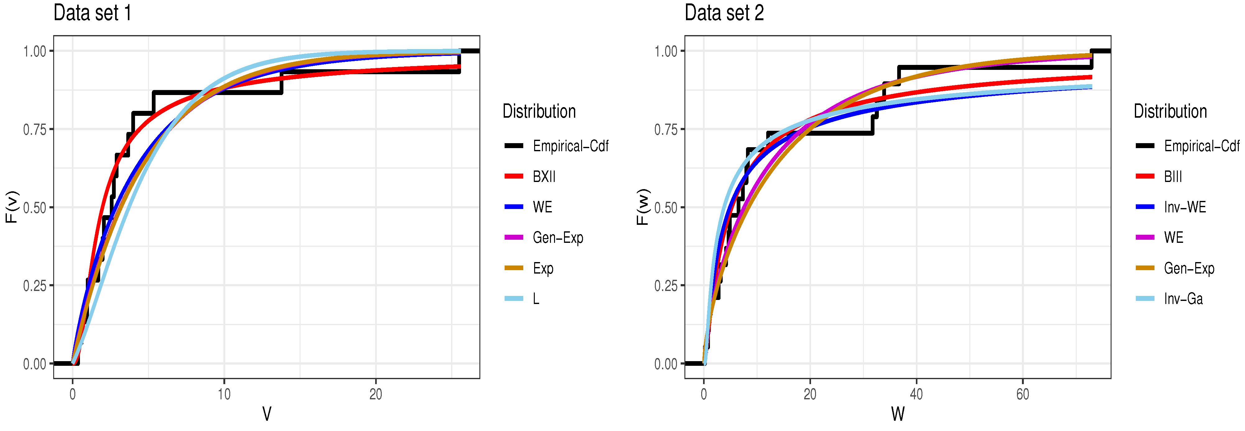
The BXII$(\vartheta ,{\phi }_1)$ and BIII$(\vartheta ,{\phi }_2)$ distributions are initially applied independently to datasets V and W. First and foremost, it is crucial to ascertain the suitability of each distribution to analyze its respective dataset. This involves computing the MLEs for the parameters and assessing various goodness-of-fit criteria, including the negative log-likelihood criterion (NLC), the Akaike information criterion value (AICV), the Bayesian information criterion value (BICV), and the Anderson–Darling test (ADT) statistics, as well as the Kolmogorov–Smirnov test (K-ST) statistic and its corresponding p-value. These criteria are subsequently compared with those obtained from alternative distributions. For Dataset 1 with the BXII distribution, the alternatives include Weibull (WE), generalized exponential (Gen-Exp), exponential (Exp), and Lindely (L) distributions. As for Dataset 2, the compared distributions with BIII are inverse Weibull (Inv-WE), WE, Gen-Exp, and inverse gamma (Inv-Ga). Lower values of these criteria, coupled with larger p-values, indicate a superior fit. The findings, encompassing parameter estimates and goodness-of-fit statistics, are detailed in Table 6. The results from Table 6 indicate that, among the distributions considered, BXII and BIII serve as appropriate models for the provided Dataset 1 and Dataset 2, respectively. Additionally, Figure 3 presents visualizations of empirical and fitted distribution functions. These visuals distinctly highlight that the BXII and BIII distributions exhibit a more favorable alignment with Dataset 1 and Dataset 2, respectively, in comparison to the other distributions under consideration. This observation holds true, at least within the confines of these specific datasets.

Table 6. Evaluation of the goodness of fit for the provided two datasets.

Dataset	PDF	Estimate		NLC	AICV	BICV	ADT	K-ST	p-Value
V	BXII	2.4589	0.3766	36.2367	76.4735	77.8896	0.2885	0.1721	0.7045
	WE	0.8890	4.2915	37.6914	79.3828	80.7989	0.6647	0.1917	0.5751
	Gen-Exp	0.9650	4.7197	37.9052	79.8103	81.2264	0.7322	0.2181	0.4143
	Exp	4.6063	---	37.9104	77.8207	78.5288	0.7299	0.2205	0.4006
	L	0.3750	---	39.8715	81.7431	82.4512	0.8948	0.2703	0.1854
W	BIII	0.8260	3.0670	1.6263	7.2526	9.1415	0.4151	0.1235	0.9003
	Inv-WE	1.9279	0.6434	70.6897	145.3795	147.2683	0.6187	0.1579	0.6738
	WE	0.7705	12.2139	68.3860	140.7721	142.6609	0.4804	0.1611	0.6499
	Gen-Exp	0.6829	18.6776	68.6489	141.2978	143.1867	0.4908	0.1886	0.4535
	Inv-Ga	0.5301	0.9645	72.1593	148.3187	150.2076	0.8862	0.2164	0.2917

Figure 3. The empirical distribution function and fitted distribution functions for Datasets 1 and 2.

Next, we check whether the null hypothesis $H_0:{\vartheta }_{\mathrm{Data}\mathrm{W}}={\vartheta }_{\mathrm{Data}\mathrm{V}}$ against the alternative $H_1:{\vartheta }_{\mathrm{Data}\mathrm{W}}\ne {\vartheta }_{\mathrm{Data}\mathrm{V}}$ holds. In this scenario, we calculate the test statistic as

$$-2\left[{\ell }^{*}\left({\widehat{\vartheta }}_{\mathrm{Data}\mathrm{W}},{\widehat{\varphi }}_2\right)-{\ell }^{*}\left({\widehat{\vartheta }}_{\mathrm{Data}\mathrm{V}},{\widehat{\varphi }}_1\right)\right]=69.2209,$$

and its associated p-value is found to be less than 0.05. Consequently, we accept the null hypothesis, affirming the validity of the assumption $H_0:{\vartheta }_{\mathrm{Data}\mathrm{W}}={\vartheta }_{\mathrm{Data}\mathrm{V}}$.

With the initial pair of datasets, we produce two sets of TII-PC samples from each dataset. These samples are constructed with a varying number of stages, precisely $m=10$, adhering to the item removal scheme outlined in Table 7.

Table 7. Generated m data of the TII-PC and corresponding censored schemes.

i	1	2	3	4	5	6	7	8	9	10
$v_i$	0.35	0.96	1.69	1.97	2.07	2.71	2.90	3.67	3.99	5.35
$R_i$	1	2	1	1	0	0	0	0	0	0
$w_i$	0.19	1.31	2.78	4.15	4.67	4.85	7.35	8.27	12.06	31.75
$R_i^{\circ }$	2	2	2	1	1	1	0	0	0	0

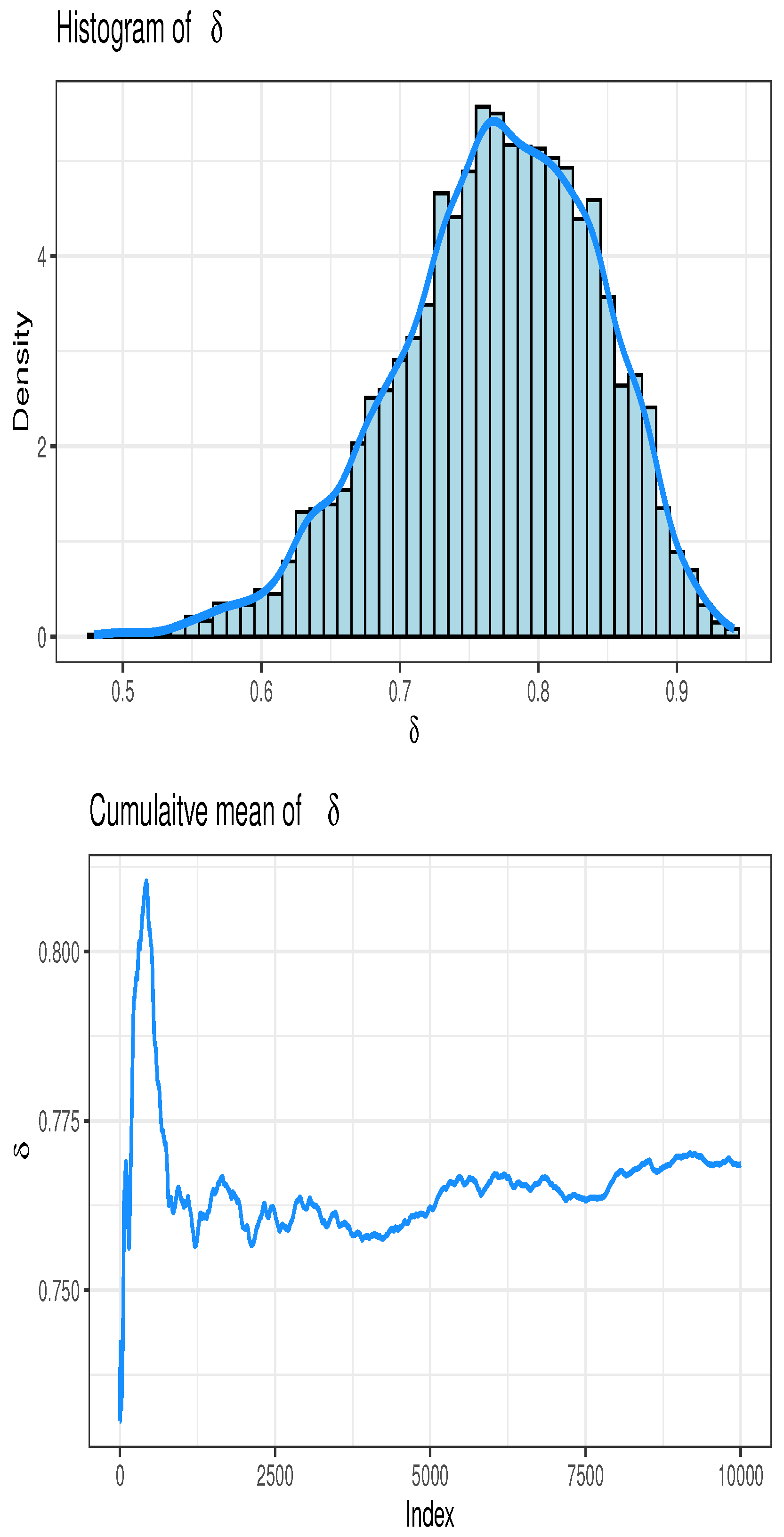
We compute the estimate of $\delta$ through MLE for the parameters $\vartheta ,{\phi }_1$, and ${\phi }_2$, considering varying TII-PC patterns based on the provided two real datasets (V and W). The estimated value is found to be 0.7307. Furthermore, we calculate BEs using MCMC and utilizing the MH algorithm with the N-INF prior. While generating samples from the posterior distribution using MH, we initialize the value of $\delta$ as ${\delta }^{\left(0\right)}=\widehat{\delta }$, where $\widehat{\delta }$ represents the MLE of $\delta$. Subsequently, we discard the initial 2000 burn-in samples from a total of 10,000 samples generated from the posterior density. BEs are then derived using different loss functions, including SEF and LNx (with $\alpha =-1.5$ for $LN{x}_1$ and $\alpha =1.5$ for $LN{x}_2$). The obtained BEs for SEF, $LN{x}_1$ and $LN{x}_2$ are 0.7709, 0.7667, and 0.7750, respectively.

Finally, the convergence of MCMC estimates using the MH algorithm for $\delta$ can be illustrated in Figure 4. This set of figures includes a trace plot, histogram, and cumulative mean for the estimated parameter $\delta$ under N-INF priors. These visualizations illustrate the normality of the generated posterior samples for the parameter $\delta$ and convergence to approximately 0.76.

Figure 4. Convergence of MCMC samples for $\delta$.

7. Conclusions

Progressive censoring is frequently used in life testing and reliability studies to address a variety of issues that experimenters have while conducting various sorts of experiments, including cutting down on overall test duration, saving experimental units, and estimating effectively. One sort of progressive censoring that has been created to enable removal with specified distribution is the TII-PC with random removal. In this work, the estimate of the SS model is based on the assumption that the distributions of the random variables for stress and strength are distinct with common shape parameters. The point estimator for $\delta$ is generated using the TII-PC with binomial removal, taking the ML and Bayesian techniques into consideration. The MCMC approach and the MH algorithm, based on symmetric and asymmetric loss functions, are both carried out in light of INF and N-INF priors and result in Bayesian estimates. The effectiveness of the generated estimates is validated by a comprehensive simulation analysis. We discovered that the Bayes estimates employing the MCMC approach outperformed MLEs. Therefore, when analyzing data, one may consider using the Bayesian approach using the MH algorithm if prior knowledge about the data is available; otherwise, one may use ML or the Bayesian method based on the N-INF prior. Finally, to illustrate how our SS reliability model problem may be applied, we take a look at a real-world case.

References

- Kotz, S.; Pensky, M. The Stress-Strength Model and Its Generalizations: Theory and Applications; World Scientific: Singapore, 2003. [Google Scholar]
- Awad, A.M.; Gharraf, M.K. Estimation of P(Y < X) in the Burr case: A comparative study. Commun. Stat.-Simul. Comput. 1986, 15, 389–403. [Google Scholar] [CrossRef]
- Ahmed, K.E.; Fakhry, M.E.; Jaheen, Z.F. Empirical Bayes estimation of R=P(Y<X) and characterizations of Burr-type X model. J. Stat. Plan. Inference 1997, 64, 297–308. [Google Scholar]
- Kundu, D.; Gupta, R.D. Estimation of P[Y < X] for generalized exponential distribution. Metrika 2005, 61, 291–308. [Google Scholar] [CrossRef]
- Rezaei, S.; Tahmasbi, R.; Mahmoodi, M. Estimation of P[Y < X] for generalized Pareto distribution. J. Stat. Plan. Inference 2010, 140, 480–494. [Google Scholar] [CrossRef]
- Panahi, H.; Asadi, S. Estimation of R = P[Y<X] for two-parameter Burr Type XII Distribution. World Acad. Sci. Eng. Technol. 2010, 72, 465–470. [Google Scholar]
- Asgharzadeh, A.; Valiollahi, R.; Raqab, M.Z. Stress-strength reliability of Weibull distribution based on progressively censored samples. SORT-Stat. Oper. Res. Trans. 2011, 35, 103–124. [Google Scholar]
- Saracoğlu, B.; Kinaci, I.; Kundu, D. On estimation of R = P(Y < X) for exponential distribution under progressive type-II censoring. J. Stat. Comput. Simul. 2012, 82, 729–744. [Google Scholar] [CrossRef]
- Yadav, A.S.; Singh, S.K.; Singh, U. Estimation of stress–strength reliability for inverse Weibull distribution under progressive type-II censoring scheme. J. Ind. Prod. Eng. 2018, 35, 48–55. [Google Scholar] [CrossRef]
- Shoaee, S.; Khorram, E. Stress–strength reliability of a two-parameter Bathtub-shaped lifetime distribution based on progressively censored samples. Commun. Stat. Methods 2015, 44, 5306–5328. [Google Scholar] [CrossRef]
- Abd-Elfattah, A.M.; Abu-Moussa, M.H.; El-Fahham, M.M. Estimation of Stress-Strength Parameter for Burr type XII distribution Based on progressive type-II Censoring. In Proceedings of the 1st International Conference on New Horizons in Basic and Applied Science, Hurghada, Egypt, November 2013; Volume 1. Available online: http://www.anglisticum.mk (accessed on 20 October 2023).
- Yousef, M.M.; Hassan, A.S.; Alshanbari, H.M.; El-Bagoury, A.-A.H.; Almetwally, E.M. Bayesian and Non-Bayesian Analysis of Exponentiated Exponential Stress–Strength Model Based on Generalized Progressive Hybrid Censoring Process. Axioms 2022, 11, 455. [Google Scholar] [CrossRef]
- de la Cruz, R.; Salinas, H.S.; Meza, C. Reliability Estimation for Stress–Strength Model Based on Unit-Half-Normal Distribution. Symmetry 2022, 14, 837. [Google Scholar] [CrossRef]
- Temraz, N.S.Y. Inference on the stress strength reliability with exponentiated generalized Marshall Olkin-G distribution. PLoS ONE 2023, 18, e0280183. [Google Scholar] [CrossRef]
- Kumar, I.; Kumar, K.; Ghosh, I. Reliability Estimation in Inverse Pareto Distribution Using Progressively First Failure Censored Data. Am. J. Math. Manag. Sci. 2023, 42, 126–147. [Google Scholar] [CrossRef]
- Alsadat, N.; Hassan, A.S.; Elgarhy, M.; Chesneau, C.; Mohamed, R.E. An Efficient Stress–Strength Reliability Estimate of the Unit Gompertz Distribution Using Ranked Set Sampling. Symmetry 2023, 15, 1121. [Google Scholar] [CrossRef]
- Yu, Y.; Wang, L.; Dey, S.; Liu, J. Estimation of stress-strength reliability from unit-Burr III distribution under records data. Math. Biosci. Eng. 2023, 20, 12360–12379. [Google Scholar] [CrossRef]
- Kamel, I.; Anwar, T.; Najim, A. Different estimation methods of reliability in stress-strength model under chen distribution. AIP Conf. Proc. 2023, 2591, 050023. [Google Scholar] [CrossRef]
- Hassan, A.S.; Almanjahie, I.M.; Al-Omari, A.I.; Alzoubi, L.; Nagy, H.F. Stress–strength modeling using median- ranked set sampling: Estimation, simulation, and application. Mathematics. 2023, 11, 318. [Google Scholar] [CrossRef]
- Balakrishnan, N.; Aggarwala, R. Progressive Censoring: Theory, Methods, and Applications; Springer Science & Business Media: Boston, MA, USA, 2000. [Google Scholar]
- Balakrishnan, N. Progressive censoring methodology: An appraisal. TEST 2007, 16, 211–296. [Google Scholar] [CrossRef]
- Yuen, H.K.; Tse, S.K. Parameters estimation for Weibull with random removals. J. Stat. Comput. Simul. 1996, 55, 57–71. [Google Scholar] [CrossRef]
- Amin, Z.H. Bayesian inference for the Pareto lifetime model under progressive censoring with binomial removals. J. Appl. Stat. 2008, 35, 1203–1217. [Google Scholar] [CrossRef]
- Wu, S.J.; Chen, Y.J.; Chang, C.T. Statistical inference based on progressively censored samples with random removals from the Burr type XII distribution. J. Stat. Comput. Simul. 2007, 77, 19–27. [Google Scholar] [CrossRef]
- Tse, S.K.; Yang, C.; Yuen, H.K. Statistical analysis of Weibull distributed lifetime data under type-II progressive censoring with binomial removals. J. Appl. Stat. 2000, 27, 1033–1043. [Google Scholar] [CrossRef]
- Dey, S.; Dey, T. Statistical Inference for the Rayleigh distribution under progressively Type-II censoring with binomial removal. Appl. Math. Model. 2014, 38, 974–982. [Google Scholar] [CrossRef]
- Yan, W.; Shi, Y.; Song, B.; Zhaoyong, H. Statistical analysis of generalized exponential distribution under progressive censoring with binomial removals. J. Syst. Eng. Electron. 2011, 22, 704–714. [Google Scholar] [CrossRef]
- Mokhlis, L.S.D.; Khames, S.K.; Sadk, S.W. Estimation of Stress-Strength Reliability for Marshall- Olkin Extended Weibull Family Based on Type-II Progressive Censoring. J. Stat. Appl. Probab. 2021, 10, 385–396. [Google Scholar]
- Burr, W.I. Cumulative frequency distribution. Ann. Math. Stat. 1942, 13, 215–232. [Google Scholar] [CrossRef]
- Burr, I.W.; Cislak, P.J. On a general system of distributions: I. Its curve-shape characteristics; II. The sample median. J. Am. Stat. Assoc. 1968, 63, 627–635. [Google Scholar] [CrossRef]
- Tadikamalla, P.R. A look at the Burr and related distributions. Int. Stat. Rev./Revue Int. Stat. 1980, 48, 337–344. [Google Scholar] [CrossRef]
- Chou, C.Y.; Cheng, P.H.; Liu, H.R. Economic statistical design of X charts for non-normal data by considering quality loss. J. Appl. Stat. 2000, 27, 939–951. [Google Scholar] [CrossRef]
- Jones, A.M.; Lomas, J.; Nigel, R. Applying beta-type size distributions to health-care cost regressions. J. Appl. Econom. 2014, 29, 649–670. [Google Scholar] [CrossRef]
- McDonald, J.B.; Richards, D.O. Model selection, some generalized distributions. Commun. Stat. Theory Methods 1987, 16, 1049–1074. [Google Scholar] [CrossRef]
- Mielke, P.W., Jr.; Johnson, E.S. Some generalized beta distributions of the second kind having desirable applications features in hydrology and meterology. Water Resour. Res. 1974, 10, 223–226. [Google Scholar] [CrossRef]
- Wingo, D.R. Maximum likelihood methods for fitting the Burr type-XII distribution to life test data. Biom. J. 1983, 25, 77–81. [Google Scholar] [CrossRef]
- Cook, D.R.; Johnson, E.S. Generalized Burr-Pareto-Logistic distributions with applications to a uranium exploration data set. Technometrics 1986, 28, 123–131. [Google Scholar] [CrossRef]
- Li, X.; Shi, Y.; Wei, J.; Chai, J. Empirical Bayes estimators of reliability performances using LINEX loss under progressively type-II censored samples. Math. Comput. Simul. 2007, 73, 320–326. [Google Scholar] [CrossRef]
- Abd-Elfattah, A.M.; Hassan, A.S.; Nassr, S.G. Estimation in step-stress partially accelerated life tests for the Burr Type XII distribution using type I censoring. Stat. Methodol. 2008, 5, 502–514. [Google Scholar] [CrossRef]
- Rastogi, M.K.; Tripathi, Y.M. Estimating a parameter of Burr type XII distribution using hybrid censored observations. Int. J. Qual. Reliab. Manag. 2011, 28, 885–893. [Google Scholar] [CrossRef]
- Panahi, H.; Sayyareh, A. Estimation and prediction for a unified hybrid-censored Burr Type XII distribution. J. Stat. Comput. Simul. 2016, 86, 55–73. [Google Scholar] [CrossRef]
- Rastogi, M.K.; Tripathi, Y.M. Inference on unknown parameters of a Burr distribution under hybrid censoring. Stat. Pap. 2013, 54, 619–643. [Google Scholar] [CrossRef]
- Panahi, H. Estimation for the parameters of the Burr type XII distribution under doubly censored sample with application to microfluidics data. Int. J. Syst. Assur. Eng. 2019, 10, 510–518. [Google Scholar] [CrossRef]
- Hassan, A.S.; Assar, A.M.; Ali, K.A.; Nagy, H.F. Estimation of the density and cumulative distribution functions of the exponentiated Burr XII distribution. Stat. Transit. New Ser. 2021, 22, 171–189. [Google Scholar] [CrossRef]
- Gove, J.H.; Ducey, M.J.; Leak, W.B.; Zhang, L. Rotated sigmoid structures in managed uneven-aged northern hardwood stands: A look at the Burr Type III distribution. Forestry 2008, 81, 161–176. [Google Scholar] [CrossRef]
- Mielke, P.W. Another family of distributions for describing and analyzing precipitation data. J. Appl. Meterol. 1973, 12, 275–280. [Google Scholar] [CrossRef]
- Nadarajah, S.; Kotz, S. On the alternative to the Weibull function. Eng. Fract. Mech. 2007, 74, 451–456. [Google Scholar] [CrossRef]
- Hassan, A.S.; Elsherpieny, E.A.; Aghel, W.E. Statistical inference of the Burr Type III distribution under joint progressively Type-II censoring. Sci. Afr. 2023, 21, e01770. [Google Scholar] [CrossRef]
- Kleiber, C.; Kotz, S. Statistical Size Distributions in Economics and Actuarial Sciences; John Wiley & Sons, Inc.: Hoboken, NJ, USA, 2003. [Google Scholar]
- Altindag, O.; Cankaya, M.N.; Yalcinkaya, A.; Aydoğdu, H. Statistical inference for the Burr Type III Distribution under Type II Censored Data. Commun. Fac. Sci. Univ. Ank.-Ser. A1 Math. Stat. 2017, 66, 297–310. [Google Scholar]
- Panahi, H. Estimation of the Burr type III distribution with application in unified hybrid censored sample of fracture toughness. J. Appl. Stat. 2017, 44, 2575–2592. [Google Scholar] [CrossRef]
- Gamchi, F.V.; Alma, Ö.G.; Belaghi, R.A. Classical and Bayesian inference for Burr type III distribution based on progressive type II hybrid censored data. Math. Sci. 2019, 13, 79–95. [Google Scholar] [CrossRef]
- Hassan, A.S.; Selmy, A.S.; Assar, S.M. Assessing the Lifetime Performance Index of Burr Type III Distribution under Progressive Type II Censoring. Pak. J. Stat. Oper. Res. 2021, 17, 633–647. [Google Scholar] [CrossRef]
- Zellner, A. Bayesian estimation and prediction using asymmetric loss functions. J. Am. Stat. Assoc. 1986, 81, 446–451. [Google Scholar] [CrossRef]
- Dey, S.; Dey, T.; Luckett, D.J. Statistical inference for the generalized inverted exponential distribution based on upper record values. Math. Comput. Simul. 2016, 120, 64–78. [Google Scholar] [CrossRef]
- Balakrishnan, N.; Sandhu, R.A. A Simple Simulational Algorithm for Generating Progressive Type-II Censored Samples. Am. Stat. 1995, 49, 229–230. [Google Scholar]
- Nelson, W. Applied Life Data Analysis; Wiley: New York, NY, USA, 1982. [Google Scholar]
Disclaimer/Publisher’s Note: The statements, opinions and data contained in all publications are solely those of the individual author(s) and contributor(s) and not of MDPI and/or the editor(s). MDPI and/or the editor(s) disclaim responsibility for any injury to people or property resulting from any ideas, methods, instructions or products referred to in the content. |
© 2023 by the authors. Licensee MDPI, Basel, Switzerland. This article is an open access article distributed under the terms and conditions of the Creative Commons Attribution (CC BY) license (https://creativecommons.org/licenses/by/4.0/).