Uniformly Shifted Exponential Distribution

Abstract

The use of life distributions has increased over the past decade, receiving particular attention in recent years, both from a practical and theoretical point of view. Life distributions can be used in a number of applied fields, such as medicine, biology, public health, epidemiology, engineering, economics, and demography. This paper presents and investigates a new life distribution. The proposed model shows favorable characteristics in terms of reliability theory, which makes it competitive against other commonly used life distributions, such as the exponential, gamma, and Weibull distributions. The methods of maximum likelihood and moments are used to estimate the parameters of the proposed model. Additionally, real-life data drawn from different fields are used to illustrate the usefulness of the new distribution. Further, the R programming language is used to perform all computations and produce all graphs.

1. Introduction

The use of life distribution models increased in the late 20th century, mainly because they proved to be flexible for use with a wide variety of random phenomena, and because of rapid innovations in computing power. The statistical analysis of lifetime data, sometimes referred to as survival time or failure time data, is important in many fields, including in biomedicine, engineering, social sciences, medicine, biology, public health, epidemiology, engineering, economics, and demography [1]. In the 1970s, interest in life distribution grew quickly in terms of theory, methodology, and application, and from the 1980s onwards, software programs for lifetime data analysis became readily accessible. Indeed, new features and packages are now added on a regular basis [1].

One of the most important theories associated with life distribution models is reliability theory, which was conceived in the late 1940s and early 1950s [2]. Reliability theory concerns the study of the lifespan of the components of equipment or systems, as well as their failure or non-failure rates over time. Indeed, reliability theory is an important part of statistical research about reliability [2]. Further, ordering distributions and log concavity properties, especially among lifetime distributions, have a significant impact on the statistical literature, particularly when it comes to reliability theorem and its applications [3]. For example, an extensive discussion on the ordering of different life distributions is presented in [4,5]. Also, a discussion about the log-concavity for several life distributions, including extreme-value, exponential, Weibull, power function, gamma, log-normal, Student’s t, and more, is seen in [6]. The log-concavity property of a life distribution has practical applications in economics, social sciences, information theory, and optimization. The field of information economics especially deals with the assumption that the log of the cumulative distribution function is a concave function. Moreover, the log-concavity of survival functions is crucial in reliability theory, since it corresponds to an increasing or decreasing failure rate. Fortunately, most of life distributions have a concave cumulative function.

In the 1930s and 1940s, univariate life distributions were commonly used in the field of statistics, but serious research about these distribution only really began in about 1950 [1]. Among the univariate models, a few distributions occupy a central position because of their usefulness in a wide range of situations. The most popular life distributions used are exponential, Weibull, log-normal, log-logistic, and gamma distributions. In 1939, the Weibull distribution began to be used to test the strength or fatigue life of materials [2]. Later, in 1956 and 1959, the Weibull distribution was employed in reliability theory, and in medicine in 1966 [1]. In recent years, the Weibull distribution has become increasingly popular for analyzing lifetime data, because it is considerably easier to manage, at least computationally, than gamma distribution, in the presence of censoring. Nevertheless, one disadvantage of using the Weibull distribution is that maximum likelihood (ML) estimator distribution reveals a slower asymptotic convergence to normality; indeed, unless the sample size is sufficiently high, it is probable that the majority of asymptotic inferences will be inaccurate. The Weibull distribution also lacks any ordering properties, in contrast to gamma distribution, for example [7].

Gamma distribution has been used for many years, and its use demonstrates a number of positive features [4]. Gamma distribution enables considerable amounts of flexibility for analyzing positive real-world data, especially life data. It has an increasing and decreasing failure rate based on shape parameter, giving it an advantage over exponential distribution, which shows constant failure rates. Another interesting feature of gamma distribution is that when the scale parameter remains constant, it shows likelihood ratio ordering, with regard to shape parameter. Also, gamma distribution can be used in areas other than lifetime distributions. For example, [8,9,10] examine gamma distribution in relation to failure times. However, if the shape parameter is not an integer, the distribution function, or survival function, cannot be defined in a closed form, which is a significant disadvantage of gamma distribution. As a result, gamma distribution is used less than Weibull distribution, which has a reasonable distribution function, survival function, and hazard function [7].

Exponential distribution is used extensively to model lifetime data, both in theory and in practice [3]. It is highly amenable to statistical studies, because it contains just one parameter, and is simple to describe. Also, in comparison to alternative life data distributions, such as Weibull distribution, it has a constant hazard rate function. A significant amount of statistical analysis and life data modeling is undertaken using exponential distribution, especially in relation to reliability, and, therefore, it is a well-established model [1]. Even though distributions such as Weibull have gained popularity, reliability engineers tend to favor exponential distribution. For example, in [11], exponential distribution is linked to reliability theory, and [12] uses exponential distribution to model medical survival statistics. The exponential model produces useful results [13], and, therefore, it is not surprising that it is still used frequently.

The motivation for this study is from the increasing popularity of lifetime data applications. The standard life distributions, such as exponential, gamma, Weibull, and others, have good properties and can model a variety of data. However, there are real-life data where such common life distributions fail to give a good fit. Hence there is a need to develop new distributions that demonstrate superior performance. The goal of this paper is to devise a novel life data distribution which performs better than current popular models, such as exponential, gamma, Weibull, etc. In addition, the objective of this study is to provide a novel life distribution that possesses favorable characteristics, particularly in reliability theory, such as ordering distribution and log concavity properties. These properties make the proposed distribution very desired for a wide range of applications across various fields. As a result, a new lifetime distribution is proposed and investigated that is referred to as uniformly shifted exponential distribution (USED). It results from the convolution of exponential and uniform distributions. The current study examines the structural characteristics of the new distribution model, including its distribution function, survival function, hazard function, and stochastic ordering. The new distribution is capable of modeling data with an increasing failure rate, and the shape of the failure rate function remains constant. The value of the new distribution is demonstrated by means of application to a real-world dataset. The rest of the paper unfolds as follows: Section 2 presents the theory behind the new model and outlines its most important statistical properties. Section 3 discusses the parameter estimations of the new model and presents a simulation study. Section 4 details real-life data applications. Finally, Section 5 concludes the paper.

2. Uniformly Shifted Exponential Distribution (USED)

In this section, uniformly shifted exponential distribution (USED) is introduced. The probability density function (pdf), cumulative distribution function, survival function, and failure rate function of the USED can be derived as follows:

If we consider that $X$ is a random variable and has exponential distribution with the rate parameter $\theta$, denoted by $X~Exp\left(\theta \right)$, and $U$ is an independent random variable, which has uniform distribution on the interval $[0,a]$ ($U~U\left(0,a\right))$, then the random variable $Y=X+U$ has the following probability density function:

$$\begin{array}{ll}f\left(y\right)& ={\int }_0^{\min \left(y,a\right)}\frac{\theta }{a}{e}^{-\theta \left(y-u\right)}du=\frac{1}{a}\left(e^{-\theta \left(y-\min \left(y,a\right)\right)}-e^{-\theta y}\right)\\ & =\frac{1}{a}\left\{\begin{array}{l}1-e^{-\theta y}, y\le a\\ e^{-\theta \left(y-a\right)}-e^{-\theta y}, y>a\end{array}\right.\\ & =\frac{1}{a}\left[\delta \left(y\right)(1-e^{-\theta y})+(1-\delta \left(y\right))(e^{-\theta \left(y-a\right)}-e^{-\theta y})\right], y>0\end{array}$$

(1)

Here, $\delta \left(y\right)=1$ for $y\le a$ and 0 for $y>a>0$.

Definition 1. 

The random variable   $Y$  is said to have uniformly shifted exponential distribution with the parameters   $a>0$   and   $\theta >0$  ($USED(a, \theta ))$  if its pdf is given by (1).

Additionally, the properties outlined below can be derived from Definition 1:

Proposition 1. 

If   $Y~USED(a, \theta )$, then the cumulative distribution function (cdf), the survival function (sf), and the failure rate function (fr), respectively, can be given as follows:

$$F(y)=\frac{1}{a}\left\{\begin{array}{c}y-\frac{1}{\theta }(1-e^{-\theta y}), y\le a\\ a-\frac{1}{\theta }\left(e^{-\theta \left(y-\mathrm{a}\right)}-e^{-\theta y}\right), y>a,\end{array}\right.$$

(2)

$$sf(y)=1-F\left(y\right)=\frac{1}{a}\left\{\begin{array}{c}a-y+\frac{1}{\theta }(1-e^{-\theta y}), y\le a\\ \frac{1}{\theta }\left(e^{-\theta \left(y-\mathrm{a}\right)}-e^{-\theta y}\right), y>a,\end{array}\right.$$

(3)

and

$$fr(y)=\left\{\begin{array}{c}{\left(\frac{a-y}{1-e^{-\theta y}}+\frac{1}{\theta }\right)}^{-1}, y\le a\\ \theta , y>a\end{array}\right.$$

(4)

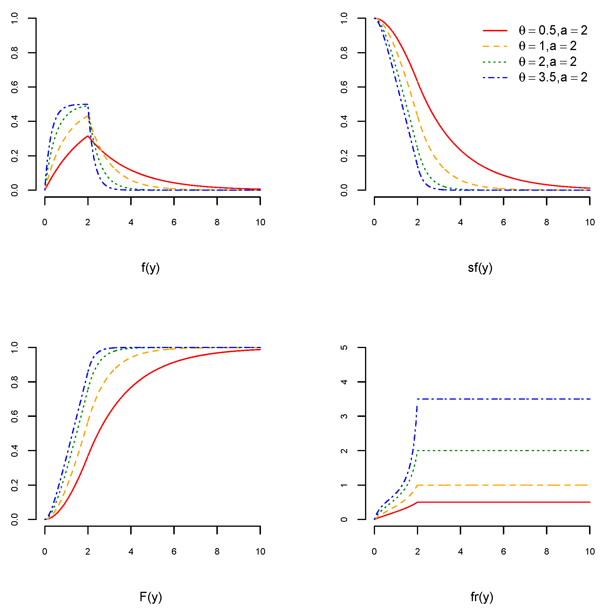
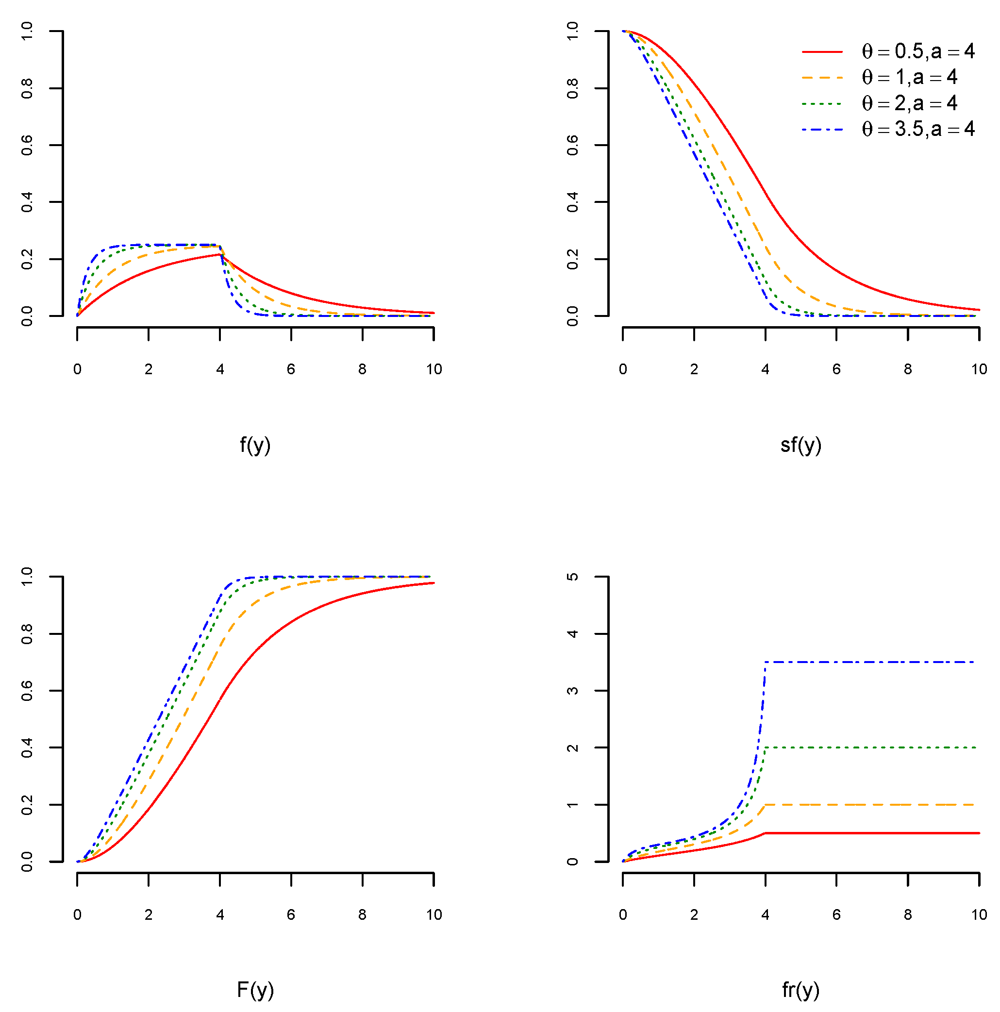
Here, fr remains constant when $Y$ is greater than $a$. Figure 1, Figure 2 and Figure 3 visualize the graphs of pdf, cdf, sf, and fr of the USED for different values of $a$ and $\theta .$ We can see in Figure 1, Figure 2 and Figure 3 (top left) that the pdfs of the USED are skewed to the right. For $Y<a$, the pdfs of the USED become more concave, and for $Y>a$, they become less convex. Figure 1, Figure 2 and Figure 3 (bottom right) show that the fr of the USED remains constant when $Y\ge a$ and it increases for $Y\le a$.

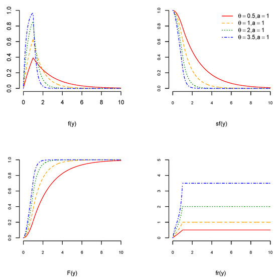
Figure 1. The pdf of the USED (top left), the cdf of the USED (bottom left), the sf of the USED (top right), and the fr of the USED (bottom right) when $a=1$ and for $\theta =0.5, 1, 2,$ and 3.5.

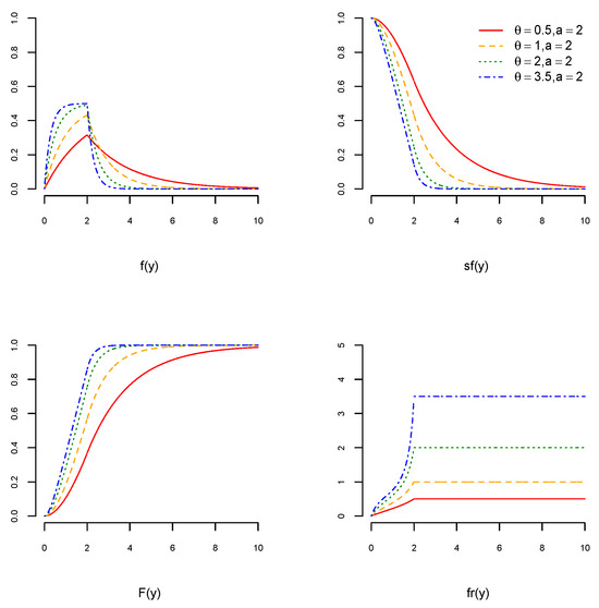
Figure 2. The pdf of the USED (top left), the cdf of the USED (bottom left), the sf of the USED (top right), and the fr of the USED (bottom right) when $a=2$ and for $\theta =0.5, 1, 2,$ and 3.5.

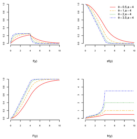
Figure 3. The pdf of the USED (top left), the cdf of the USED (bottom left), the sf of the USED (top right), and the fr of the USED (bottom right) when $a=4$ and for $\theta =0.5, 1, 2$, and 3.5.

Remark 1. 

If we re-parametrize the USED, and set   $\theta =\eta /a$, then the following applies:

$$f(y;a,\eta )=\frac{1}{a}\left\{\begin{array}{c}1-e^{-\frac{\eta }{a}y}, y\le a\\ e^{-\frac{\eta }{a}\left(y-\mathrm{a}\right)}-e^{-\frac{\eta }{a}y}, y>a\end{array}\right.$$

Note that

$$af(ay;a,\eta )=\left\{\begin{array}{c}1-e^{-\eta y}, y\le 1\\ e^{-\eta \left(y-1\right)}-e^{-\eta y}, y>1\end{array}\right.$$

which is USED (1, $\eta$), and, hence, $a$ can be viewed as a scale parameter.

2.1. Statistical Properties

This section reviews the statistical results relating to moments associated with the USED. Further, stochastic orders are addressed, and the properties of the USED as they relate to reliability theory are discussed.

2.1.1. The Moments of the USED

Proposition 2. 

If   $Y~USED(a, \theta )$, then the non-central moments of order n (${\mu }_n)$   can be given as follows:

$${\mu }_n=\frac{n!}{{\theta }^n}{\sum }_{k=0}^n\frac{{\left(a\theta \right)}^k}{(k+1)!}, 0<\theta <\theta <\infty , n=1, 2, \dots$$

(5)

Proof. 

From the definition of the non-central moments, we obtain the following:

$$\begin{array}{ll}{\mu }_n=E\left(Y^n\right)=E\left({\left(U+X\right)}^n\right)& ={\displaystyle \sum _{k=0}^n}\left(\genfrac{}{}{0pt}{}{n}{k}\right)E\left(U^k\right)E\left(X^{n-k}\right)\\ & ={\sum }_{k=0}^n\frac{n!}{k!\left(n-k\right)!}\frac{a^k}{k+1}\frac{\left(n-k\right)!}{{\theta }^{n-k}}\\ & =\frac{n!}{{\theta }^n}{\sum }_{k=0}^n\frac{{\left(a\theta \right)}^k}{\left(k+1\right)!}\end{array}$$

This delivers the desired outcome.□

From Proposition 2, the mean and the variance of the USED can be defined as follows:

Corollary 1. 

The mean   $\mu$  and the variance   ${\sigma }^2$  of the USED, respectively, are

$$\mu =\frac{a}{2}+\frac{1}{\theta }$$

(6)

and

$${\sigma }^2=\frac{a^2}{12}+\frac{1}{{\theta }^2}$$

(7)

Proposition 3. 

$$4{\sigma }^2\ge {\mu }^2$$

Proof. 

From Corollary 1, we obtain the following:

$$4{\sigma }^2-{\mu }^2=\frac{a^2}{3}+\frac{4}{{\theta }^2}-{\left(\frac{a}{2}+\frac{1}{\theta }\right)}^2$$

Then,

$$\begin{array}{ll}4{\sigma }^2-{\mu }^2& =\frac{a^2}{12}+\frac{3}{{\theta }^2}-\frac{a}{\theta }\\ & =\frac{a^2}{{12\gamma }^2}({\gamma }^2-12\gamma +36)=\frac{a^2}{{12\gamma }^2}{(\gamma -6)}^2\end{array}$$

Here, $\gamma =a\theta$. This is clearly non-negative, with a zero value when $a\theta =6$. This completes the proof. □

2.1.2. Reliability and Stochastic Order

Log-concavity probability distributions play a vital role in many applications, such as reliability theory, labor economics, monopoly theory, mechanism design theory, political science, and law, among others. See [6] for more details. The log-concave function of the USED can be defined as follows:

Definition 2. 

A function f is said to be log-concave for the interval   $(a,b)$  if the function   $ln\left(f\right)$   is a concave function of   $\left(a,b\right).$

Due to the fact that the USED is a convolution of two log-concave distributions, which are uniform and exponential distributions, its pdf is log concave and, thus, it is strongly unimodal [14]. The log-concavity of the pdfs implies that the cdfs and sfs are, likewise, log-concaves [6]. This means that the USED incorporates an increasing failure rate function (IFR) [5]. The log-concavity and IFR are two critical features in reliability theory which give the USED its value in reliability applications.

Many different stochastic orderings are used by statistical researchers. The four most popular ones are the likelihood ratio (${\le }_{lr})$, hazard rate (${\le }_{hr})$, stochastic ordering (${\le }_{st})$, and variability ordering (${\le }_v)$. Likelihood ratio ordering is the strongest order, in the sense that it implies the other three orderings. For more detail, see, for example [5]. The definition of the likelihood ratio can be given as follows:

Definition 3. 

Let   $X$  and   $Y$   be two random variables with corresponding pdfs, namely   $f$  and   $g$, such that   $f\left(x\right)/g\left(x\right)$   decreases  in x on the union of the supports of   $X$  and   $Y$. Then,   $X$   can be said to be smaller than   $Y$   in the likelihood ratio order (denoted by   $X{\le }_{lr}Y$).

Many classes of probability distributions, such as exponential and Poisson models, are likelihood-ordered with respect to their parameters. The USED shows favorable stochastic orders, as stated in the following proposition:

Proposition 4. 

If   $Y_1~USED(a,{ \theta }_1)$  and   $Y_2~USED(a,{ \theta }_2)$, then   $Y_1\le Y_2$  for   ${ \theta }_1\le { \theta }_2.$

Proof. 

It can be observed that  $Y_i=X_i+U, i=\mathrm{1,2}$  with  $X_i~Exp\left({ \theta }_i\right)$  are independent and identical to  $U$. In addition, it is known that  $X_1{\ge }_{lr}{X}_2$  and  $U$  has log-concave density [15,16]. Therefore,  $X_1+U{\ge }_{lr}{X}_2+U$, which completes the proof. □

Proposition 5. 

If   $Y_1~USED(a_1,\theta )$   and   $Y_2~USED(a_2,\theta )$, then   $Y_1{\le }_{lr}$  $Y_2$  for   ${ a}_1<{ a}_2.$

Proof. 

Let $Y_i=X+U_i, i=\mathrm{1,2}$, where $U_i~U\left(0,a_i\right)$ is independent and identical to $X~Exp\left(\theta \right)$. Here, the union of the support points of the two uniform distributions is ${(0, a}_2)$. Thus, if we denote as $f_i\left(y\right)$ the pdf of $U_i$, we obtain the following:

$$f_1\left(y\right)/f_2\left(y\right)=\left\{\begin{array}{c}\frac{a_2}{a_1}, 0<{y<a}_1\\ 0 , a_1\le {y<a}_2\end{array},\right.$$

The above decreases in ${(0, a}_2)$. Therefore, according to Definition 2, we obtain $U_1{\le }_{lr}{U}_2$. It can be seen that the exponential distribution has a log-concave pdf, and therefore, an argument similar to that used to prove Proposition 4 offers the required result. □

3. Parameter Estimation and Simulation

This section presents the parameter estimation and a simulation study, both of which are important steps for understanding and evaluating the proposed model. For the parameter estimation, classical methods of estimation were used, namely, the maximum likelihood (ML) method and the method of moments (MM). In addition, a simulation was conducted to gain insight into the results obtained. The statistical programming language R (R core Team) was used to calculate the ML and MM estimates. It is worth mentioning here that two cases were considered and examined in order to obtain the USED parameters, when parameter $a$ is known and unknown.

3.1. Parameter Estimation

3.1.1. Maximum Likelihood Estimation (ML)

As demonstrated in many studies undertaken in the field of statistics, ML is one of the most widely used parametric estimation methods. In ML, estimation is driven by the maximization of the likelihood function (L), which frequently satisfies regularity conditions. In the context of the current study, let $Y={(Y}_1, Y_2,\dots ,Y_n)$ be a random sample of size $n$ from the USED, with the unknown parameters $a$ and $\theta$, and $y=(y_1, y_2,\dots ,y_n)$ be the $n$ observed values. Here, $L$ is given as follows:

$$\begin{array}{ll}L\left(a,\theta , y\right)={\prod }_{i=1}^{n}f\left(y_i\right)& =\frac{1}{a^n}{\prod }_{i=1}^n{(1-e^{-\theta y_i})}^{\delta \left(y_i\right)}{e}^{-\theta y_i\left(1-\delta \left(y_i\right)\right)}{(e^{\theta a}-1)}^{\left(1-\delta \left(y_i\right)\right)}\\ & =\frac{1}{a^n}{\displaystyle \prod _{i=1}^{n_1}}{(1-e^{-\theta y_i})}^{\delta \left(y_i\right)}{\displaystyle \prod _{i=1}^{n_2}}{e}^{-\theta y_i\left(1-\delta \left(y_i\right)\right)}{(e^{\theta a}-1)}^{\left(1-\delta \left(y_i\right)\right)}\\ & =\frac{{(e^{\theta a}-1)}^{n_2}}{a^n}{\displaystyle \prod _{i=1}^{n_1}}{(1-e^{-\theta y_i})}^{\delta \left(y_i\right)}{\displaystyle \prod _{i=1}^{n_2}}{e}^{-\theta y_i\left(1-\delta \left(y_i\right)\right)}\end{array}$$

Here, $\delta \left(y_i\right)=1$ for $y_i\le a$ and 0 for $y_i>a>0$. $n_1$ is the number of observed values that satisfy $y_i\le a$, and $n_2$ refers to the number of observed values for which $y_i>a$, where $n=n_1+n_2$.

It is worth noting that $f\left(y_i\right)$ is differentiable at all $y_i$ except at $y_i=a.$ The ML estimators of $a$ and $\theta$ are the values that maximize the log likelihood function ($\mathcal{l})$, which are denoted as $\widehat{a}$ and $\widehat{\theta }$, respectively. The corresponding $\mathcal{l}$ can be defined as follows:

$$\mathcal{l}=\mathit{log}L\left(a,\theta , y \right)=n_2\mathit{log}{(e}^{\theta a}-1)-n\mathit{log}\left(a\right)+{\sum }_{i=1}^{n_1}\delta \left(y_i\right)\mathit{log}\left(1-e^{-\theta y_i}\right)-\theta {\sum }_{i=1}^{n_2}{y}_i\left(1-\delta \left(y_i\right)\right)$$

(8)

Below, two cases relating to the USED parameters are discussed:

(a)

Case 1: the parameter $a$ is known:

In this case, the ML estimate $\widehat{\theta }$ is obtained by differentiating the function $\mathcal{l}$ in (8) with respect to $\theta$ and solving the following score function:

$$\frac{\partial \mathcal{l}}{\partial \theta }=\frac{\partial logL\left(\theta ,\mathit{y} \right)}{\partial \theta }=n_2\frac{a{e}^{\widehat{\theta }a}}{e^{\widehat{\theta }a}-1}+{\sum }_{i=1}^n\delta \left(y_i\right)\frac{{y_{i}e}^{-\widehat{\theta }{y}_i}}{1-e^{-\widehat{\theta }{y}_i}}-{\sum }_{i=1}^n\left(1-\delta \left(y_i\right)\right)y_i=0$$

(9)

Since the closed-form expression for the ML estimate $\widehat{\theta }$ cannot be found by solving (9), a nonlinear optimization algorithm is required.

(b)

Case 2: the parameter $a$ is unknown

In this case, the ML estimates $\widehat{a}$ and $\widehat{\theta }$ cannot be calculated by differentiating (8) with respect to $a$ and $\theta$ because the function $\mathcal{l}$ is not differentiable with respect to $a.$ As a result, a mathematical method developed by Nelder and Mead [17] was used to obtain the ML estimates $\widehat{a}$ and $\widehat{\theta }$. This method is robust and performs effectively with respect to non-differentiable functions. Further details can be found in [17].

3.1.2. The Method of Moments (MM)

Another well-known parametric estimation technique is the MM, which involves replacing population moments with sample moments to drive the estimators. In the current study for MM, two cases of the parameter $a$ were addressed as follows:

(a)

Case 1: the parameter $a$ is known:

The following equation was considered in order to estimate the parameter $\theta$ as follows:

$$\overline{x}=\frac{1}{\widehat{\theta }}+\frac{a}{2}$$

The following equation is the MM estimate of $\widehat{\theta }$:

$$\widehat{\theta }=\frac{2}{2\overline{x}-a}$$

(b)

Case 2: the parameter $a$ is unknown.

The MM estimates $\widehat{a}$ and $\widehat{\theta }$ can be obtained by solving the coupled equations below:

$$\overline{x}=\frac{1}{\widehat{\theta }}+\frac{\widehat{a}}{2}$$

and

$$\frac{{\widehat{a}}^2}{12}+\frac{1}{{\widehat{\theta }}^2}=s^2$$

By using the above equations, we obtain the following equations:

$$\widehat{a}=\frac{2(\widehat{\theta }\overline{x}-1)}{\widehat{\theta }}$$

and

$$\widehat{\theta }=\frac{-\overline{x}\pm \sqrt{{3(4s}^2-{\overline{x}}^2)}}{\left(3s^2-{\overline{x}}^2\right)}$$

(10)

Using (14), the condition for a real solution can be given as follows:

$${4s}^2-{\overline{x}}^2\ge 0$$

(11)

If (15) offers a real solution, it is possible to discriminate between two situations: the first is where one of the solutions is negative and will thus be rejected, and the second is as follows:

$${3s}^2-{\overline{x}}^2\ge 0$$

In the second situation, we have ${3s}^2-{\overline{x}}^2\le 0$, and both solutions are positive. This is clear for the root $\frac{-\overline{x}-\sqrt{{3(4s}^2-{\overline{x}}^2)}}{\left(3s^2-{\overline{x}}^2\right)}$, and for the root $\frac{-\overline{x}+\sqrt{{3(4s}^2-{\overline{x}}^2)}}{\left(3s^2-{\overline{x}}^2\right)}.$ It should be noted that under the assumption ${3s}^2-{\overline{x}}^2\le 0$, $-\overline{x}+\sqrt{{3(4s}^2-{\overline{x}}^2)}\le -\overline{x}$$+\sqrt{3s^2}\le 0$ as $3s^2-{\overline{x}}^2=(\sqrt{3s^2}-\overline{x})(\sqrt{3s^2}+\overline{x})$.

Finally, a simulation analysis was conducted for the two scenarios $a$ = 2, $\theta$ = 1.5 and $a$ = 2, $\theta$ = 3.0, and the results revealed that the MM estimators were unreliable, as expected.

Therefore, for Case 2, when $a$ is unkown, the MM estimates were not included in the simulation study and the ML estimates were considered.

3.2. Simulation Study

This sub-section presents a numerical evaluation of the proposed parameter estimators. A simulation study was performed to examine the performance of the ML and MM estimates of the USED parameters $a$ and $\theta$. A total of 1000 Monte Carlo replications with sample sizes of $n=$ 20, 50, 200, and 1000 were considered. Random samples, such that $Y~$USED ($a$, $\theta$), were generated using one of the following Algorithms 1 and 2:

Algorithm 1:

Choose the values $a$ and $\theta$ and the sample size $n$. Generate $n$ random samples, such that $U~$Unif (0, $a$). Generate $n$ random samples, such that $X~$Exp($\theta$). Compute $Y=X+U$.

Algorithm 2:

Choose the values $a$ and $\theta$ and the sample size $n.$ Generate $n$ random samples, such that $U~$Unif (0, $1$). Set $y=F^{-1}\left(u\right)$ and then $u=F\left(y\right).$ From Step 3, $Y$ can be obtained as a solution of one of the following cases: i. If $u<1-\frac{1}{a\theta }(1-e^{-\theta a})$, then the equation $u=\frac{1}{a}[y-\frac{1}{\theta }\left(1-e^{-\theta y}\right)]$ can be solved numerically to obtain $Y$. ii. For $u\ge 1-\frac{1}{a\theta }(1-e^{-\theta a})$, we have $u=1-\frac{1}{a\theta }{e}^{-\theta y}(e^{\theta a}-1)$. Hence, $y=-\frac{1}{\theta }\ln a\theta \frac{1-u}{e^{\theta a}-1}$.

In practice, the two algorithms did not show a significant difference. Therefore, for simplicity, Algorithm 1 was performed. The mean square error (MSE) of the estimated parameters and the associated bias were used as assessment criteria, with the following formula:

$$\mathrm{bias}=\frac{\sum _{i=1}^n(\alpha -{\widehat{\alpha }}_i)}{n}$$

Here, ${\widehat{\alpha }}_i$ is the estimate of $\alpha$ at the i-th replication, and

$$\mathrm{MSE}=\frac{\sum _{i=1}^n{(\alpha -{\widehat{\alpha }}_i)}^2}{n}$$

Table 1, Table 2, Table 3 and Table 4 show the MSE and bias of $\widehat{\theta }$ when $a$ is known. In general, the MSE of the ML estimates were less than the MSE of the MM estimates, especially for small sample size such as $n$ = 20, and large values of $a$ and $\theta$. In addition, the bias of the ML estimates was smaller than the bias of the MM estimates in most cases, indicating that the ML estimation of the USED parameters yielded good precision, as expected. Table 1, Table 2, Table 3 and Table 4 show that all estimates are asymptotically unbiased, because as $n$ increases with the bias approaching 0, the MSEs decrease to 0.

Table 1. MSE and bias for the USED estimates by ML and MM, when $a$ = 1 with $\theta$ = 0.5, 1, 2, and 3.5 and n = 20, 50, 200, and 1000.

$\mathit{a}=1$
$\mathit{\theta }$	$\mathit{n}$	20		50		200		1000
	Method	ML	MM	ML	MM	ML	MM	ML	MM
0.5	MSE	0.0168	0.0169	0.0052	0.0052	0.0015	0.0015	0.0002	0.0002
	Bias	−0.0297	−0.0293	−0.0107	−0.0105	−0.0044	−0.0042	0.0001	0.0001
1	MSE	0.0766	0.0771	0.0266	0.0267	0.0056	0.0056	0.0009	0.0009
	Bias	−0.0721	−0.0707	−0.0272	−0.0265	−0.0043	−0.0038	−0.0007	−0.0004
2	MSE	0.3995	0.4284	0.1219	0.1261	0.0250	0.0267	0.0053	0.0058
	Bias	−0.1514	−0.1341	−0.0506	−0.0474	−0.0113	−0.0108	−0.0046	−0.0052
3.5	MSE	0.8240	31.0637	0.4343	0.7724	0.1080	0.1302	0.0212	0.0251
	Bias	−0.2160	−0.7623	−0.1078	−0.1513	−0.0486	−0.0426	−0.0045	−0.0031

Table 2. MSE and bias for the USED estimates by ML and MM, when $a$ = 2 with $\theta$ = 0.5, 1, 2, and 3.5 and n = 20, 50, 200, and 1000.

$\mathit{a}=2$
$\mathit{\theta }$	$\mathit{n}$	20		50		200		1000
	Method	ML	MM	ML	MM	ML	MM	ML	MM
0.5	MSE	0.0204	0.0202	0.0062	0.0062	0.0014	0.0014	0.0003	0.0003
	Bias	−0.0425	−0.0411	−0.0113	−0.0107	−0.0043	−0.0039	−0.0008	−0.0009
1	MSE	0.1058	0.1176	0.0299	0.0328	0.0060	0.0065	0.0013	0.0014
	Bias	−0.0770	−0.0750	−0.0276	−0.0261	−0.0039	−0.0036	0.0002	0.0007
2	MSE	0.7988	19.1086	0.2161	0.2467	0.0409	0.0552	0.0074	0.0094
	Bias	−0.2934	−0.5663	−0.0938	−0.0826	−0.0269	−0.0244	−0.0033	−0.0030
3.5	MSE	1.0941	6664.5272	0.6678	33.0863	0.2115	0.4176	0.0383	0.0666
	Bias	−0.2243	1.9524	−0.1825	−0.7256	−0.0670	−0.0818	−0.0054	−0.0083

Table 3. MSE and bias for the USED estimates by ML and MM, when $a$ = 4 with $\theta$ = 0.5, 1, 2, 3.5, and n = 20, 50, 200, and 1000.

$\mathit{a}=4$
$\mathit{\theta }$	$\mathit{n}$	20		50		200		1000
	Method	ML	MM	ML	MM	ML	MM	ML	MM
0.5	MSE	0.0234	0.0261	0.0082	0.0087	0.0017	0.0018	0.0003	0.0003
	Bias	−0.0353	−0.0334	−0.0172	−0.0156	−0.0042	−0.0038	−0.0010	−0.0009
1	MSE	0.3984	11.2194	0.0577	0.0766	0.0107	0.0134	0.0019	0.0026
	Bias	−0.1919	−0.3197	−0.0559	−0.0536	−0.0167	−0.0165	−0.0027	−0.0040
2	MSE	1.7473	14,413.1539	0.6515	36.5301	0.0736	0.1613	0.0145	0.0286
	Bias	−0.5622	−4.7084	−0.2696	−0.6382	−0.0396	−0.0670	−0.0089	−0.0132
3.5	MSE	1.5399	4029.6126	1.0440	1744.6145	0.3780	7.1093	0.0765	0.2679
	Bias	−0.4296	−2.4414	−0.2790	−1.3159	−0.1110	−0.5041	−0.0353	−0.0663

Table 4. MSE and bias for the USED estimates by ML and MM, when $a$ = 10 with $\theta$ = 0.5, 1, 2, 3.5, and n = 20, 50, 200, and 1000.

$\mathit{a}=10$
$\mathit{\theta }$	$\mathit{n}$	20		50		200		1000
	Method	ML	MM	ML	MM	ML	MM	ML	MM
0.5	MSE	0.4206	57.0900	0.0179	0.0264	0.0034	0.0049	0.0006	0.0008
	Bias	−0.1765	0.2161	−0.0316	−0.0302	−0.0080	−0.0082	−0.0012	−0.0011
1	MSE	2.2529	573.4089	0.3256	10.5837	0.0273	0.0896	0.0046	0.0109
	Bias	−0.6463	0.1299	−0.1635	−0.0889	−0.0356	−0.0741	−0.0063	−0.0103
2	MSE	4.2206	2169.5671	1.8487	2296.9807	0.2655	529.9422	0.0359	0.1718
	Bias	−1.2000	−0.9169	−0.6100	0.2995	−0.1221	−1.1577	−0.0248	−0.0690
3.5	MSE	2.0887	4043.8915	1.5151	1686.1875	0.7667	2375.4158	0.1952	6.9258
	Bias	−0.5933	5.9748	−0.3372	4.0644	−0.2123	2.0774	−0.0759	−0.5657

It can be observed that as $a$ and $\theta$ increase, the MSE and the bias of both the ML and MM estimates increase, which offers the insight that the USED is adequate to fit data with small $a$s and $\theta$s.

The MSE and bias of $\widehat{\theta }$ and $\widehat{a}$ when $a$ is unknown are shown in Table 5, Table 6, Table 7 and Table 8, from which it can be seen that the MSE of the ML estimates $\widehat{a}$ and $\widehat{\theta }$ decreases as $n$ increases. This proves that the estimates are consistent. Furthermore, the effect of $a$ and $\theta$ on the ML estimates $\widehat{a}$ and $\widehat{\theta }$ is that the MSEs and biases become bigger for large values of $a$ and $\theta$, as in the case when $a$ is known, which leads to the same conclusion.

Table 5. MSE and bias for the USED estimates by ML, when $a$ is unknown with $\theta$ = 0.5, 1, 2, 3.5, and n = 20, 50, 200, and 1000.

$\mathit{a}=1$
$\mathit{\theta }$	$\mathit{n}$	20		50		200		1000
	Method	$\widehat{\mathit{\theta }}$	$\widehat{\mathit{a}}$	$\widehat{\mathit{\theta }}$	$\widehat{\mathit{a}}$	$\widehat{\mathit{\theta }}$	$\widehat{\mathit{a}}$	$\widehat{\mathit{\theta }}$	$\widehat{\mathit{a}}$
0.5	MSE	0.0726	0.3519	0.0099	0.1456	0.0603	0.0681	0.0003	0.0052
	Bias	−0.0764	−0.1502	−0.0247	−0.0736	−0.0609	−0.0307	−0.0008	−0.0034
1	MSE	35.5560	0.1543	0.0603	0.0681	0.0093	0.0156	0.0017	0.0031
	Bias	−0.3634	−0.0749	−0.0609	−0.0307	−0.0095	−0.0068	−0.0010	0.0002
2	MSE	229.9456	0.0786	0.5708	0.0388	0.0677	0.0095	0.0104	0.0017
	Bias	−2.1569	−0.0351	−0.2019	−0.0197	−0.0519	−0.0066	−0.0092	−0.0001
3.5	MSE	3158.8143	0.0427	347.1037	0.0206	0.4078	0.0058	0.0475	0.0009
	Bias	−9.6112	−0.0166	−1.4488	−0.0121	−0.1003	0.0017	−0.0186	−0.0006

Table 6. MSE and bias for the USED estimates by ML, when $a$ is unknown with $\theta$ = 0.5, 1, 2, 3.5, and n = 20, 50, 200, and 1000.

$\mathit{a}=2$
$\mathit{\theta }$	$\mathit{n}$	20		50		200		1000
	Method	$\widehat{\mathit{\theta }}$	$\widehat{\mathit{a}}$	$\widehat{\mathit{\theta }}$	$\widehat{\mathit{a}}$	$\widehat{\mathit{\theta }}$	$\widehat{\mathit{a}}$	$\widehat{\mathit{\theta }}$	$\widehat{\mathit{a}}$
0.5	MSE	21.9504	0.6313	0.0840	0.3337	0.0026	0.0721	0.0004	0.0118
	Bias	−0.3004	−0.1701	−0.0447	−0.0998	−0.0092	−0.0298	−0.0016	−0.0023
1	MSE	537.1179	0.3160	0.0883	0.1430	0.0162	0.0370	0.0026	0.0069
	Bias	−1.8255	−0.0656	−0.0847	−0.0596	−0.0253	−0.0154	−0.0041	−0.0040
2	MSE	2108.3841	0.1511	384.0509	0.0704	0.1053	0.0181	0.0155	0.0030
	Bias	−9.0006	−0.0395	−1.4898	−0.0192	−0.0620	−0.0060	−0.0086	−0.0001
3.5	MSE	6785.7681	0.0744	8724.5597	0.0410	0.6612	0.0101	0.0806	0.00162
	Bias	−25.0450	0.0011	−11.1737	0.0057	−0.1852	0.0013	−0.03164	−0.00001

Table 7. MSE and bias for the USED estimates by ML, when $a$ is unknown with $\theta$ = 0.5, 1, 2, 3.5, and n = 20, 50, 200, and 1000.

$\mathit{a}=4$
$\mathit{\theta }$	$\mathit{n}$	20		50		200		1000
	Method	$\widehat{\mathit{\theta }}$	$\widehat{\mathit{a}}$	$\widehat{\mathit{\theta }}$	$\widehat{\mathit{a}}$	$\widehat{\mathit{\theta }}$	$\widehat{\mathit{a}}$	$\widehat{\mathit{\theta }}$	$\widehat{\mathit{a}}$
0.5	MSE	760.6967	1.2599	0.0683	0.6139	0.0035	0.1388	0.0006	0.0252
	Bias	−1.9175	−0.1920	−0.0642	−0.1142	−0.0103	−0.0187	−0.0019	−0.0042
1	MSE	1665.0231	0.5054	9.2068	0.2621	0.0276	0.0735	0.0045	0.0132
	Bias	−5.9667	−0.1062	−0.2850	−0.0682	−0.0314	−0.0066	−0.0076	0.0005
2	MSE	3384.1277	0.2823	443.2164	0.1261	0.2564	0.0329	0.0295	0.0053
	Bias	−18.7055	0.0145	−3.7381	−0.0128	−0.1243	0.0039	−0.0183	0.0039
3.5	MSE	8964.8755	0.1565	10,717.823	0.064	1.3577	0.0170	0.1579	0.0027
	Bias	−35.4863	0.0731	−23.307	0.001	−0.3123	0.0053	−0.0605	0.0013

Table 8. MSE and bias for the USED estimates by ML, when $a$ is unknown with $\theta$ = 0.5, 1, 2, 3.5, and n = 20, 50, 200, and 1000.

$\mathit{a}=10$
$\mathit{\theta }$	$\mathit{n}$	20		50		200		1000
	Method	$\widehat{\mathit{\theta }}$	$\widehat{\mathit{a}}$	$\widehat{\mathit{\theta }}$	$\widehat{\mathit{a}}$	$\widehat{\mathit{\theta }}$	$\widehat{\mathit{a}}$	$\widehat{\mathit{\theta }}$	$\widehat{\mathit{a}}$
0.5	MSE	146.3037	2.7509	42.1854	1.3567	0.0092	0.3202	0.0015	0.0681
	Bias	−3.2340	−0.2228	−0.7593	−0.1219	−0.0248	−0.0254	−0.0027	0.0100
1	MSE	479.0844	1.1676	308.5340	0.6163	0.0823	0.1579	0.0089	0.0248
	Bias	−10.1092	−0.0323	−3.8132	−0.0571	−0.0781	−0.0114	−0.0080	0.0012
2	MSE	4596.2101	0.4562	2518.1247	0.2963	200.7502	0.0784	0.0799	0.0128
	Bias	−29.1971	−0.0610	−17.3501	0.0122	−1.2515	0.0068	−0.0332	0.0055
3.5	MSE	19,761.6465	0.3257	4710.8936	0.1996	2059.2400	0.0410	0.6099	0.0071
	Bias	−44.1650	0.1582	−30.7075	0.0883	−6.6763	0.0126	−0.1976	−0.0025

4. Applications

This section presents a comparison of the USED with other competing models, in order to demonstrate the practical effectiveness of the USED. Its real-life applications are analyzed to evaluate the performance of the USED. The comparison of the fitted models is based on conventional metrics, namely, the Akaike information criterion (AIC), the Bayesian information criterion (BIC), and the function $\mathcal{l}$. In practical terms, the formulas for the AIC and BIC can be given, respectively, as follows:

$$\mathrm{AIC}=-2{\mathcal{l}}^{*}+2r$$

and

$$\mathrm{BIC}=-2{\mathcal{l}}^{\mathit{*}}+r\mathit{log}(n)$$

Here, ${\mathcal{l}}^{*}$ is the estimation of the log likelihood $\mathcal{l},$ and $r$ is the number of parameters.

4.1. Eruption Data for the Kiama Blowhole

The Kiama Blowhole is a popular tourist destination located approximately 120 km south of Sydney, in Australia. The waiting times between the Kiama Blowhole’s 65 successive eruptions comprise the data used to test the USED model proposed in the current study. Kiama Blowhole eruptions are caused by rising ocean levels, which forces water into a hole behind a cliff, which then erupts through an exit, drowning everything in its path. From 12 July 1998, a digital watch was employed to track the time between eruptions over a 1340 h period. These data are used by [18] to test the performance of the Harris extended exponential distribution (HEED), which is compared to other models, such as the exponentiated Weibull model, the Marshall–Olkin extended exponential model, the exponentiated exponential model, and Weibull and gamma distributions. The study in [18] claims that the HEED is better than its competing models for fitting data based on the AIC and BIC. In [18], the pdf of the HEED is expressed as follows:

$$f_2\left(y;k,{\beta }_2, {\lambda }_2\right)=\frac{{\lambda }_2{{\beta }_2}^{\frac{1}{k}}{e}^{-{\lambda }_{2}y}}{{\left[1-\left(1-{\beta }_2\right)e^{-{\lambda }_{2}ky}\right]}^{1+\frac{1}{k}}}; y, k,{\beta }_2, {\lambda }_2>0$$

For the current study, the USED was fitted to the same data and compared with the models used in [18]. Table 9 summarizes the fittings results for the USED and HEED. The results are shown in terms of the number of parameters used, and according to the AIC, BIC, and ${\mathcal{l}}^{*}$. The results show that the USED is better than the HEED for fitting the real data based on the BIC and AIC, and better than the other models, namely, exponential, gamma, and Weibull distributions, according to the AIC, BIC, and ${\mathcal{l}}^{*}$.

Table 9. The ML-estimated fitting parameters of the waiting times of eruptions of the Kiama Blowhole, using the exponential, gamma, Weibull, USED, and HEED models, along with their goodness-of-fit.

Model	Exponential	Gamma		Weibull		USED		HEED
ML estimates	Rate	Shape	Rate	Scale	Shape	$\widehat{\theta }$	$\widehat{a}$	$\widehat{k}$	${\widehat{\beta }}_2$	${\widehat{\lambda }}_2$
	0.03	1.62	0.04	43.21	1.27	0.03	9	19.64	22.39	0.03
BIC	603.78	600.11		602.12		594.14		597.41
AIC	601.63	595.80		597.80		589.82		590.94
${\mathcal{l}}^{*}$	−299.81	−295.90		−296.90		−292.90		−292.47

4.2. The Waiting Times for Bank Customers

The data used here relate to the amount of time in minutes 100 customers wait to be served at the branch of a bank. The study [19] uses these data to investigate how well the Lindley distribution fits the data in comparison to exponential distribution. According to the ${\mathcal{l}}^{*}$ and the P-P plot and Q-Q plot, [19] indicates that the Lindley distribution fits the data better than the other models used. The current study examines the AIC, BIC, and ${\mathcal{l}}^{*}$ for the USED against traditional life distributions, including the Lindley distribution. The findings for data fitting for the USED, exponential, gamma, Weibull, and Lindley models are summarized in Table 10. Based on the AIC and ${\mathcal{l}}^{*}$ only, the results demonstrate that the USED fits real data better than the Lindley distribution. In addition, the USED is better than all other models when taking into account every criterion.

Table 10. The ML-estimated fitting parameters of the waiting times for bank customers, using the USED, exponential, gamma, Weibull, and Lindley models, along with their goodness-of-fit.

Model	Exponential	Gamma		Weibull		USED		Lindley
ML estimates	rate	shape	rate	scale	shape	$\widehat{\theta }$	$\widehat{a}$	$\widehat{\lambda }$
	0.101	2.01	0.20	10.95	1.46	0.13	4.70	0.187
BIC	662.64	643.81		646.67		643.15		642.61
AIC	660.04	638.60		641.46		637.94		640
${\mathcal{l}}^{*}$	−329.02	−317.3		−318.73		−316.97		−319

4.3. Students’ Scores in Mathematics

One of the most well-known technical institutions in India, the Indian Institute of Technology Kanpur, provides the data used here. The Joint Entrance Examination (JEE) is used for first-year admissions to various disciplines. Every year, about 450 students enroll for their first year at the institute. However, students have the option of selecting a slow-paced program, because, often, the work is extremely challenging and competitive. All courses are required to be completed by all students in their first year. By the first mid-term exam, students may choose to enroll in a slow-paced program if they receive a sub-par grade in a particular subject; this mark varies from subject to subject and is not fixed each year. The following data comprise the final exam scores for students who studied mathematics at a slow pace in 2003:

29, 25, 50, 15, 13, 27, 15, 18, 7, 7, 8, 19, 12, 18, 5, 21, 15, 86, 21, 15, 14, 39, 15, 14, 70, 44, 6, 23, 58, 19, 50, 23, 11, 6, 34, 18, 28, 34, 12, 37, 4, 60, 20, 23, 40, 65, 19, 31.

The study [20] uses these data to investigate whether or not the weighted exponential distribution (WE) better fits the data in comparison to the Weibull, gamma, and extended exponential distributions. According to [20], the ${\mathcal{l}}^{*}$ and the Kolmogorov–Smirnov test statistic (KS) indicate that the WE distribution fits the data better than the exponential distribution. For the current study, the fitting results for the exponential, gamma, Weibull, USED, and WE models are summarized in Table 11. According to the findings, the USED fits the real data more accurately than any other model when considering the AIC, BIC, and ${\mathcal{l}}^{*}$.

Table 11. The ML-estimated fitting parameters of the students’ scores in mathematics, using the USED, exponential, gamma, Weibull, and WE models, along with their goodness-of-fit.

Model	Exponential	Gamma		Weibull		USED		WE
ML estimates	Rate	Shape	Rate	Scale	Shape	$\widehat{\theta }$	$\widehat{a}$	$\widehat{\beta }$	$\widehat{\lambda }$
	0.04	2.22	0.09	28.91	1.51	0.05	15	0.44	0.07
BIC	412.26	401.94		404.29		400.08		402.24
AIC	410.39	398.19		400.55		396.34		398.49
${\mathcal{l}}^{*}$	−204.20	−197.09		−198.28		−196.17		−197.25

4.4. Daily Ozone Measurements in New York

The data presented here are the daily ozone measurements in New York from May to September in 1973. In [21], the α-power transformed generalized exponential distribution (αPTGE) is compared to the modified Weibull, exponential Weibull, and extended generalized gamma distributions for fitting data. The study [21] finds that the αPTGE distribution performs better than other distributions based on the ${\mathcal{l}}^{*}$, KS test, Q-Q plot, and AIC. Table 12 presents the fitting results for the USED, exponential, gamma, Weibull, and αPTGE models. The USED outperforms all other models for fitting real data based on the AIC, BIC, and ${\mathcal{l}}^{*}$.

Table 12. The ML-estimated fitting parameters of the daily ozone data set, using the USED, exponential, gamma, Weibull, and αPTGE models, along with their goodness-of-fit.

Model	Exponential	Gamma		Weibull		USED		αPTGE
ML estimates	Rate	Shape	Rate	Scale	Shape	$\widehat{\theta }$	$\widehat{a}$	$\widehat{\gamma }$	$\widehat{\beta }$	$\widehat{\lambda }$
	0.023	1.70	0.040	46.08	1.34	0.028	15.052	0.48	1.93	0.03
BIC	1104.61	1092.58		1094.72		1089.14		1096.44
AIC	1101.85	1087.08		1089.22		1083.63		1088.18
${\mathcal{l}}^{*}$	−549.93	−541.53		−542.61		−539.82		−541.09

5. Conclusions

This paper outlined a new life distribution called the uniformly shifted exponential distribution (USED). The main advantage of the USED is its increased survival function. This advantage is valuable for fitting different kinds of real-life data. The statistical properties of the USED were outlined, and some properties of this model were proven, to show that the USED variables can be stochastically ordered. Estimation for the USED was achieved using the ML method and the MM, with different parameters. In the simulation, the ML method offered good performance for estimation when placed in comparison to the MM. Real data were used to examine the performance of the USED for fitting lifetime data, in comparison with other models. The applications show the superiority of the proposed distribution in comparison with the other models. This implies that among the common life distributions, the USED can be used as an effective alternative distribution for modeling lifetime data. Finally, although the USED was applied using data sets, the model can be generalized and utilized in other areas of research.

References

- Lawless, J.F. Statistical Models and Methods for Lifetime Data; John Wiley & Sons: Hoboken, NJ, USA, 2011. [Google Scholar]
- Lawless, J. Statistical methods in reliability. Technometrics 1983, 25, 305–316. [Google Scholar] [CrossRef]
- Marshall, A.W.; Olkin, I. Life Distributions; Springer: Berlin/Heidelberg, Germany, 2007; Volume 13. [Google Scholar]
- Johnson, N.L.; Kotz, S.; Balakrishnan, N. Continuous Univariate Distributions, Volume 2; John Wiley & Sons: Hoboken, NJ, USA, 1995; Volume 289. [Google Scholar]
- Shaked, M.; Shanthikumar, J.G. Stochastic Orders; Springer: Berlin/Heidelberg, Germany, 2007. [Google Scholar]
- Bagnoli, M.; Bergstrom, T. Log-concave probability and its applications. In Rationality and Equilibrium: A Symposium in Honor of Marcel K. Richter; Springer: Berlin/Heidelberg, Germany, 2006; pp. 217–241. [Google Scholar]
- Gupta, R.D.; Kundu, D. Exponentiated exponential family: An alternative to gamma and Weibull distributions. Biometr. J. J. Math. Methods Biosci. 2001, 43, 117–130. [Google Scholar] [CrossRef]
- Alexander, G. The Use of the Gamma Distribution in Estimating Regulated Output from Storage; State Rivers and Water Supply Commission: Melbourne, Australia, 1961. [Google Scholar]
- Epstein, B. Statistical Assessment of the Life Characteristic (A Bibliographic Guide). J. R. Stat. Soc. Ser. C Appl. Stat. 2018, 13, 56. [Google Scholar] [CrossRef]
- Cox, D.R. Renewal Theory; Chapman and Hall: Boca Raton, FL, USA, 1962. [Google Scholar]
- Davis, D. An analysis of some failure data. J. Am. Stat. Assoc. 1952, 47, 113–150. [Google Scholar] [CrossRef]
- Feigl, P.; Zelen, M. Estimation of exponential survival probabilities with concomitant information. Biometrics 1965, 21, 826–838. [Google Scholar] [CrossRef] [PubMed]
- Balakrishnan, K. Exponential Distribution: Theory, Methods and Applications; Routledge: London, UK, 2019. [Google Scholar]
- Merkle, M. Convolutions of Logarithmically Concave Functions; Publikacije Elektrotehničkog Fakulteta; Serija Matematika: Belgrade, Serbia, 1998; pp. 113–117. [Google Scholar]
- An, M.Y. Log-Concave Probability Distributions: Theory and Statistical Testing; Duke University Dept of Economics Working Paper; Duke University: Durham, NC, USA, 1997. [Google Scholar]
- Borzadaran, G.M.; Borzadaran, H.M. Log-concavity property for some well-known distributions. Surv. Math. Its Appl. 2011, 6, 203–219. [Google Scholar]
- Ja, N. A simplex algorithm for function minimization. Comput. J. 1965, 7, 308–313. [Google Scholar]
- Pinho, L.G.B.; Cordeiro, G.M.; Nobre, J.S. The Harris extended exponential distribution. Commun. Stat.-Theory Methods 2015, 44, 3486–3502. [Google Scholar] [CrossRef]
- Ghitany, M.E.; Atieh, B.; Nadarajah, S. Lindley distribution and its application. Math. Comput. Simul. 2008, 78, 493–506. [Google Scholar] [CrossRef]
- Gupta, R.D.; Kundu, D. A new class of weighted exponential distributions. Statistics 2009, 43, 621–634. [Google Scholar] [CrossRef]
- Vilca, F.; Santana, L.; Leiva, V.; Balakrishnan, N. Estimation of extreme percentiles in Birnbaum–Saunders distributions. Comput. Stat. Data Anal. 2011, 55, 1665–1678. [Google Scholar] [CrossRef]
Disclaimer/Publisher’s Note: The statements, opinions and data contained in all publications are solely those of the individual author(s) and contributor(s) and not of MDPI and/or the editor(s). MDPI and/or the editor(s) disclaim responsibility for any injury to people or property resulting from any ideas, methods, instructions or products referred to in the content. |
© 2024 by the authors. Licensee MDPI, Basel, Switzerland. This article is an open access article distributed under the terms and conditions of the Creative Commons Attribution (CC BY) license (https://creativecommons.org/licenses/by/4.0/).