Analytical Solution of Generalized Bratu-Type Fractional Differential Equations Using the Homotopy Perturbation Transform Method

Abstract

In this study, we present the generalized form of the higher-order nonlinear fractional Bratu-type equation. In this generalization, we deal with a generalized fractional derivative, which is quite useful from an application point of view. Furthermore, some special cases of the generalized fractional Bratu equation are recognized and examined. To solve these nonlinear differential equations of fractional order, we employ the homotopy perturbation transform method. This work presents a useful computational method for solving these equations and advances our understanding of them. We also plot some numerical outcomes to show the efficiency of the obtained results.

1. Introduction

Numerous areas of pure and applied mathematics focus largely on fractional calculus, which works with derivatives and integrals of arbitrary order [1,2,3,4,5]. Fractional differential equations have been used more frequently in applied mathematics and physics, as well as in the modeling and interpretation of various real-world issues. Biological science, physical science, chemical engineering, and other fields of research indicate nonlinear perspectives [6,7,8,9].

In mathematical modeling, the nonlinear fractional differential equations are quite helpful. However, it becomes more challenging to solve nonlinear systems of equations. It has been seen that there are many differential equations without an exact solution. Various innovative numerical and analytical approaches have been established to solve fractional differential equations, leading to numerical and analytical solutions to these types of problems. These techniques consist of Adomian decomposition method [10,11,12], homotopy analysis method [13,14,15]), generalized differential transform approach [16], homotopy perturbation method [17,18], modified Laplace decomposition method [19], homotopy perturbation transform method [20,21], and q-homotopy analysis transform method [22,23], etc. The homotopy perturbation method is the most effective for solving the differential equations of non-linear type because of its straightforward approach and fastest convergence rate. This technique was developed by the famous mathematician Mr. He [24,25,26]. Its main benefit is that the solution determined in series form approaches its exact solution very quickly.

Many mathematicians have developed an appropriate definition and formula for fractional calculus. Major contributions to the theory of fractional calculus with singular kernels have been made by Riemann, Caputo, Liouville, Weyl, Kilbas, and others. Gorenglo, Miller–Ross, Yang—Abdel–Cattani, Atangana–Baleanu, Wiman, and many others encouraged the study of fractional integrals and derivatives having nonsingular kernels. Miller–Ross, Yang–Abdel–Cattani, Wiman, Atangana–Baleanu, and many others promoted the study of fractional integrals and derivatives with non-singular kernels. Riemann-Liouville and Caputo are the two fractional operators that are used most frequently. However, there are several problems that are not properly described by these operators. For fractional derivatives, Caputo-Fabrizio developed a new operator in 2015 with a nonsingular kernel [27]. This nonsingular kernel makes the Caputo-Fabrizio fractional derivative stronger than the Caputo derivative.

The calculus operators of fractional type have been divided into three groups by Gomez and Atangana: weak, medium, and strong [28]. They suggest that the Riemann-Liouville fractional derivative is significantly more useful in explaining physical difficulties than the Caputo version. However, the Mittag-Leffler memory pattern of the Atangana-Baleanu fractional operator provides a good clarification. Some authors have used fractional derivatives of Atangana-Baleanu-Caputo to characterize fractional differential equations [29].

A numerical slab model of a combustion problem is examined using the Bratu-type equation [30]. Several additional issues have been solved using Bratu’s problem, such as the Chandrasekhar model, the fuel ignition model, the thermal response model, and the framework for the electrospun nano-fiber creation method [31,32]. To solve the Bratu type problem, Ghazanfari and Sephvandzadeh used the homotopy perturbation method [33], the modified variational iteration method [34], and the Adomian decomposition method [35]. Recent studies have explored numerical approaches to addressing the fractional Bratu initial value problem. Investigations have been conducted using the Bézier curve [36], the fractional differential transform method [37], and a technique grounded in the CAS wavelet scheme [38] for solving fractional Bratu-type differential equations.

Applications for nonlinear differential equations, like the Bratu-type equation, can be found in many branches of science and engineering. It is used in heat transfer to investigate temperature distributions in materials, in combustion theory to understand flame propagation, and in chemical kinetics to replicate complex reaction kinetics. The modeling of complex phenomena like population dynamics, material diffusion, reactor neutron transport, electrochemical reactions, and pollutant spread is made possible by its involvement in mathematical biology, material science, nuclear physics, electrochemistry, and environmental science. In addition to having particular uses, the Bratu-type equation is a basic mathematical model that provides an understanding of the characteristics of nonlinear differential equations. Because of this, it is a flexible and essential instrument for scientific analysis and study. The “Nonlinear Local Fractional Bratu-Type Equation” is a delightful and theoretically complex differential equation that belongs to the field of fractional calculus.

As mathematicians, physicists, and engineers grapple with issues related to non-standard calculus, nonlinear dynamics, and complex systems, they are entranced by ongoing research projects centered around the “Non-linear Local Fractional Bratu-type Equation”. Having a thorough grasp of the characteristics and solutions of this equation could improve our understanding of a variety of real-world processes and possibly lead to useful applications in fields including chemical kinetics, biological modeling, and combustion theory. In the fields of science and engineering, the Bratu-type equation is quite useful. In all domains where standard differentiable calculus is relevant, this article presents some new insights into the concept of generalization. Other expansions of the differentiability concept can be found in [39,40,41]. Very few researchers have studied the generalized form of a fractional Bratu-type equation, so finding the solution of a generalized fractional Bratu-type differential equation is a new thing in itself. Realizing how important it is, we turn our attention to examining a generalized fractional Bratu-type equation.

This study aims to define the generalized Bratu-type differential equation and expand the application of the homotopy perturbation transform method for identifying specific features of the generalized Bratu-type differential equation

$$D_t^{2n\kappa }u\left(t\right)+\delta E_{\beta }\left(u\right)=0,0<\kappa \le 1,0<t\le 1,$$

(1)

where $\delta$ is constant and $E_{\beta }\left(u\right)$ is the Mittag-Leffler function defined as

$$E_{\beta }\left(u\right)=\sum _{k=0}^{\infty }\frac{u^k}{\mathrm{\Gamma }(\beta k+1)},$$

$\mathrm{\Gamma }$ indicates the gamma function and $D^{2n\kappa }=D^{\kappa }{D}^{\kappa }\dots D^{\kappa }(2n-times)where{D}^{\kappa }u=\frac{d^{\kappa }u}{d{t}^{\kappa }}$.

The structure of this paper is divided into seven sections: We provide a brief introduction and some fundamental terminology in Section 1. The basic homotopy perturbation transform approach is defined in Section 2. In Section 3, we discuss the existence and uniqueness of the generalized fractional Bratu-type differential equation. In Section 4, we describe the main findings of this work. In Section 5, we discuss the convergence analysis. In Section 6, we describe some special cases of generalized Bratu-type equations and provide a graphic representation of the solution. This paper is concluded in the last section.

Basic Definitions

This section provides the definitions and foundational results essential for the content presented in this paper.

A theory that deals with generalized fractional-order integration and differentiation operators is called generalized fractional calculus. Using an analogy with the concept of the Caputo and R–L fractional derivative, the analogous generalized fractional derivatives are defined as [42]

$$\begin{array}{c}{ }_0^{\mathrm{C}}{\mathrm{D}}_{\mathrm{t}}^{\kappa }f\left(t\right)=\underset{0}{\overset{t}{\int }}\dot{f}\left(u\right){\Delta }_l(t-u)du,\hfill \\ { }_0{\mathrm{D}}_{\mathrm{t}}^{\kappa }f\left(t\right)=\frac{d}{dt}\underset{0}{\overset{t}{\int }}f\left(u\right){\Delta }_l(t-u)du,\hfill \end{array}$$

where $0<\kappa <1$ is the order of derivative, $f:[0,+\infty )\to \mathbb{R}$ is the absolute continuous function with $\dot{f}\in L_{\mathrm{loc}}^1(0,+\infty )$, ${\Delta }_l$ is known as the general kernel function, also for $f\in L_{\mathrm{loc}}^1(0,+\infty )$,

$${ }_0{\mathrm{D}}_{\mathrm{t}}^{-\kappa }\left[{ }_0^{\mathrm{C}}{\mathrm{D}}_{\mathrm{t}}^{\kappa }f\left(t\right)\right]=f\left(t\right)-f\left(0\right),$$

where ${ }_0{\mathrm{D}}_{\mathrm{t}}^{-\kappa }$ represent the general form of the Riemann-Liouville fractional integral defined as

$${ }_0{\mathrm{D}}_{\mathrm{t}}^{-\kappa }f\left(t\right)=\underset{0}{\overset{t}{\int }}f\left(u\right){\nabla }_l(t-u)du.$$

Definition 1. 

Caputo derivative of fractional order κ is denoted by ${ }_a^C{D}_t^{\kappa }$ and defined by [43]

$${ }_a^C{D}_t^{\kappa }f\left(t\right)=\frac{1}{\mathrm{\Gamma }(n-\kappa )}\underset{a}{\overset{t}{\int }}{(t-u)}^{n-\kappa -1}{f}^{\left(n\right)}\left(u\right)du,$$

(2)

where $0<\kappa <1andn-1<\kappa <n$. Also $f^{\left(n\right)}\left(t\right)=\frac{d^{n}f}{d{t}^n}$.

Definition 2. 

Caputo-Fabrizio derivative is denoted by ${ }_a^{CF}{D}_t^{\kappa }$ and defined by [44]

$${ }_a^{CF}{D}_t^{\kappa }f\left(t\right)=\frac{\Delta \left(\kappa \right)}{(1-\kappa )}\underset{a}{\overset{t}{\int }}exp\left[-\frac{\kappa }{(1-\kappa )}(t-u)\right]f^{\prime }\left(u\right)du,$$

(3)

where $\Delta \left(\kappa \right)$ = Normalization function with $\Delta \left(0\right)=1,\Delta \left(1\right)=1$.

Definition 3. 

We have the Atangana-Baleanu derivative which is denoted by ${ }_a^{ABC}{D}_t^{\kappa }$ and defined by [45]

$${ }_a^{ABC}{D}_t^{\kappa }f\left(t\right)=\frac{\Delta \left(\kappa \right)}{(1-\kappa )}\underset{a}{\overset{t}{\int }}{E}_{\kappa }\left[-\frac{\kappa }{(1-\kappa )}{(t-u)}^{\kappa }\right]f^{\prime }\left(u\right)du,$$

(4)

where $\mathrm{\Delta }\left(\kappa \right)$ = Normalization function with $\mathrm{\Delta }\left(0\right)=1,\mathrm{\Delta }\left(1\right)=1$ and $E_{\kappa }$ is Mittag-leffler function.

Definition 4. 

If $A=\left\{f\left(t\right)\right|\exists M,{\tau }_1,{\tau }_2>0,\left|f\left(t\right)\right|<Mexp$(^|t|/_τj), if t ∈ (−1)^j × [0,∞)} is the set of functions, then the Sumudu transform on A is defined as [46]

$$S\left[f\left(t\right)\right]\left(u\right)=\underset{0}{\overset{\infty }{\int }}{e}^{-t}f\left(ut\right)dt.$$

(5)

Definition 5. 

In accordance with the Reference [47], we define the Sumudu transform for the Caputo derivative of order $\kappa >0$

$$S\left[{ }_0^C{D}_t^{\kappa }f\left(t\right)\right]\left(s\right)=\frac{S\left[f\right]-f\left(0\right)}{s^{\kappa }}.$$

(6)

Definition 6. 

In accordance with the Reference [47], we define the Sumudu transform for the Caputo-Fabrizio derivative of order $\kappa >0$

$$S\left[{ }_0^{CF}{D}_t^{\kappa }f\left(t\right)\right]\left(s\right)=\frac{\Delta \left(\kappa \right)}{1-\kappa +\kappa s}\left(S\left[f\right]-f\left(0\right)\right),$$

(7)

where $\Delta \left(\kappa \right)$ = Normalization function with $\Delta \left(0\right)=1,\Delta \left(1\right)=1$.

Definition 7. 

In accordance with the Reference [47], we define the Sumudu transform for the Atangana-Baleanu fractional derivative of order $\kappa >0$

$$S\left[{ }_0^{ABC}{D}_t^{\kappa }f\left(t\right)\right]\left(s\right)=\frac{\Delta \left(\kappa \right)}{1-\kappa +\kappa s^{\kappa }}\left(S\left[f\right]-f\left(0\right)\right),$$

(8)

where $\Delta \left(\kappa \right)$ = Normalization function with $\Delta \left(0\right)=1,\Delta \left(1\right)=1$.

2. Basic Homotopy Perturbation Transform Approach

This section covers the Homotopy Perturbation Transform Method (HPTM) procedure for solving fractional differential equations using generalized fractional operators.

The Homotopy Perturbation Technique (HPT), incorporating He’s polynomials and a transform algorithm, is formulated as the homotopy perturbation transform method. To illustrate the fundamental workings of the homotopy perturbation transform method, we apply it to a nonlinear fractional-order differential equation of the form

$$D_t^{\kappa }u\left(t\right)+Lu\left(t\right)+Nu\left(t\right)=f\left(t\right),0<\kappa \le 1,t>0.$$

(9)

Here, u(t) represents the probability density function, $D_t^{\kappa }$ denotes the generalized fractional derivative with order $\kappa$, L stands for the linear differential operator with an order less than that of D, and N represents the general nonlinear differential operator.

Apply the Sumudu transform on both sides of (9),

$$S\left[D_t^{\kappa }u\left(t\right)\right]+S\left[Lu\left(t\right)\right]+S\left[Nu\left(t\right)\right]=S\left[f\left(t\right)\right],$$

as we know, Sumudu transform for generalized fractional derivatives [48],

$$S\left[D_t^{\kappa }u\left(t\right)\right]\left(s\right)={\varsigma }^{-1}\left[S\left[u\left(t\right)\right]-\sum _{k=0}^{n-1}{s}^k{\left[u^k\left(t\right)\right]}_{t=0}\right],0<\kappa \le 1,$$

here,

$$\begin{array}{c}\varsigma =s^{\kappa }\left(forCaputofractionalderivative\right),\hfill \\ \\ \varsigma =\frac{1-\kappa +\kappa s}{\Delta \left(\kappa \right)}(forCaputo-Fabriziofractionalderivative),\hfill \\ \\ \varsigma =\frac{1-\kappa +\kappa s^{\kappa }}{\Delta \left(\kappa \right)}(forAtangana-Baleanu-Caputofractionalderivative),\hfill \end{array}$$

and $\Delta \left(\kappa \right)$ is the normalization function.

Hence

$$S\left[u\left(t\right)\right]=\sum _{k=0}^{n-1}{s}^k{\left[u^k\left(t\right)\right]}_{t=0}-\varsigma \left\{S\left[Lu\right(t\left)\right]+S\left[Nu\right(t\left)\right]-S\left[f\right(t\left)\right]\right\}.$$

Now, applying the inverse Sumudu transform, we obtain

$$u\left(t\right)=\varphi \left(t\right)-S^{-1}\left\{\varsigma \left(S\left[Lu\right(t\left)\right]+S\left[Nu\right(t\left)\right]\right)\right\},$$

where

$$\varphi \left(t\right)=S^{-1}\left\{\sum _{k=0}^{n-1}{s}^k{\left[u^k\left(t\right)\right]}_{t=0}+\varsigma S\left[f\left(t\right)\right]\right\}.$$

Now, expanding u(t) into the series of power p as $u\left(t\right)={\displaystyle \sum _{n=0}^{\infty }}{p}^n{u}_n\left(t\right)$ and consider $Nu\left(t\right)={\displaystyle \sum _{n=0}^{\infty }}{p}^n{H}_n\left(u\right)$, here $H_n\left(u\right)$ is He’s polynomial defined as

$$H_n(u_0,u_1,u_2,\dots ,u_n)=\frac{1}{n!}\frac{\partial }{\partial p^n}{\left[N\left(\sum _{k=0}^{\infty }{p}^k{u}_k\right)\right]}_{p=0},n=0,1,2,3,\dots ,$$

and $p\in (0,1)$ is an embedding parameter.

Then

$$\sum _{n=0}^{\infty }{p}^n{u}_n\left(t\right)=\varphi \left(t\right)-p{S}^{-1}\left\{\varsigma \left(S\left[L\sum _{n=0}^{\infty }{p}^n{u}_n\left(t\right)\right]+S\left[\sum _{n=0}^{\infty }{p}^n{H}_n\left(u\right)\right]\right)\right\}.$$

(10)

This equation represents the combination of the homotopy perturbation method, He’s polynomial, and Sumudu transform.

Now, by equating the coefficients corresponding to different powers of p, we obtain

$$\begin{array}{c}{p}^0:u_0\left(t\right)=\varphi \left(t\right),\hfill \\ \\ p^1:u_1\left(t\right)=-S^{-1}\left\{\varsigma \left(S\left[L{u}_0\left(t\right)\right]+S\left[H_0\left(u\right)\right]\right)\right\},\hfill \\ \\ p^2:u_2\left(t\right)=-S^{-1}\left\{\varsigma \left(S\left[L{u}_1\left(t\right)\right]+S\left[H_1\left(u\right)\right]\right)\right\},\hfill \\ .\hfill \\ .\hfill \\ .\hfill \end{array}$$

The remaining elements of $u_n\left(t\right),n\ge 0$ can be evaluated by applying a similar approach. As a result, the homotopy perturbation transforms method solutions are completely computed.

Thus, the approximate analytical solution of (9) is

$$u\left(t\right)=\underset{p\to 1}{lim}\sum _{n=0}^{\infty }{p}^n{u}_n\left(t\right)=\sum _{n=0}^{\infty }{u}_n\left(t\right).$$

3. Existence and Uniqueness of the Solution

Theorem 1. 

The solution of the generalized Bratu-type fractional differential equation defined by (1) satisfies the Lipschitz condition and has the unique solution for $0<b<1$, where $b=\frac{\nu \left|\delta \right|}{\mathrm{\Gamma }(1+\kappa )}{t}^{\kappa }$ is known as the Lipschitz constant.

Proof. 

Firstly, we write Equation (1) in the following form

$$u\left(t\right)=-\frac{\delta }{\mathrm{\Gamma }(1+\kappa )}\underset{0}{\overset{t}{\int }}G\left(\tau ,u\left(\tau \right)\right){\left(d\tau \right)}^{\kappa }$$

(11)

where

$$G\left(t,u\left(t\right)\right)={\left(\frac{1}{\mathrm{\Gamma }(1+\kappa )}\right)}^{\left(2n-1\right)}\underset{(2n-1)times}{\underset{0}{\overset{t}{\int }}\underset{0}{\overset{t}{\int }}...\underset{0}{\overset{t}{\int }}{E}_{\beta }\left(u\left(\tau \right)\right)}{\left(d\tau \right)}^{\kappa }{\left(d\tau \right)}^{\kappa }\dots {\left(d\tau \right)}^{\kappa }$$

(12)

The non-linear part $G\left(t,u\left(t\right)\right)$ is Lipschitz continuous with the condition

$$∥G\left(t,u\right)-G\left(t,v\right)∥\le \nu ∥u-v∥.$$

(13)

Lipschitz constant can be evaluated by making use of maximum norm $∥G∥=\underset{0\le t\le 1}{max}\left|G\left(t,u\left(t\right)\right)\right|$, we have

$$\left|E_{\beta }\left(u\right)-E_{\beta }\left(v\right)\right|\le \sum _{k=0}^{\infty }\frac{\left|u^k-v^k\right|}{\mathrm{\Gamma }\left(\beta k+1\right)},$$

$$\le \sum _{k=0}^{\infty }\frac{\left|u-v\right|}{\mathrm{\Gamma }\left(\beta k+1\right)}\left|u^{k-1}+u^{k-2}v+...+u{v}^{k-2}+v^{k-1}\right|.$$

Since the series is convergent $\left|u^{k-1}+u^{k-2}v+...+u{v}^{k-2}+v^{k-1}\right|$ is bounded for each k.

Thus,

$$\left|u^{k-1}+u^{k-2}v+...+u{v}^{k-2}+v^{k-1}\right|\le M,k=1,2,3,\dots ,$$

where M is some constant.

Thus,

$$\left|E_{\beta }\left(u\right)-E_{\beta }\left(v\right)\right|\le \left|u-v\right|M\sum _{k=0}^{\infty }\frac{1}{\mathrm{\Gamma }\left(\beta k+1\right)},$$

$$\le \left|u-v\right|M{E}_{\beta }\left(1\right).$$

Now from (12), we obtain

$$\begin{array}{c}∥G\left(t,u\right)-G\left(t,v\right)∥\le {\left(\frac{1}{\mathrm{\Gamma }(1+\kappa )}\right)}^{\left(2n-1\right)}M{E}_{\beta }\left(1\right)∥u-v∥\underset{(2n-1)times}{\underset{0}{\overset{t}{\int }}\underset{0}{\overset{t}{\int }}...\underset{0}{\overset{t}{\int }}{\left(d\tau \right)}^{\kappa }}{\left(d\tau \right)}^{\kappa }\dots {\left(d\tau \right)}^{\kappa },\hfill \\ \\ ∥G\left(t,u\right)-G\left(t,v\right)∥\le {\left(\frac{1}{\mathrm{\Gamma }(1+\kappa )}\right)}^{\left(2n-1\right)}M{E}_{\beta }\left(1\right)∥u-v∥\frac{t^{(2n-1)\kappa }}{(2n-1)!},\hfill \\ \\ \le \frac{M{E}_{\beta }\left(1\right)}{(2n-1)!{\left(\mathrm{\Gamma }(1+\kappa )\right)}^{\left(2n-1\right)}}∥u-v∥.\hfill \end{array}$$

Thus, we can select the Lipschitz constant as $\nu =\frac{M{E}_{\beta }\left(1\right)}{(2n-1)!{\left(\mathrm{\Gamma }(1+\kappa )\right)}^{\left(2n-1\right)}}$.

Hence, the solution of Equation (1) exists.

Now, suppose that Equation (1) has two different solutions $u_1$ and $u_2$, so then

$$\begin{array}{c}∥u_1-u_2∥=∥\frac{\left(-\delta \right)}{\mathrm{\Gamma }(1+\kappa )}\underset{0}{\overset{t}{\int }}G\left(\tau ,u_1\left(\tau \right)\right){\left(d\tau \right)}^{\kappa }-\frac{\left(-\delta \right)}{\mathrm{\Gamma }(1+\kappa )}\underset{0}{\overset{t}{\int }}G\left(\tau ,u_2\left(\tau \right)\right){\left(d\tau \right)}^{\kappa }∥,\hfill \\ \\ \le \frac{\left|\delta \right|}{\mathrm{\Gamma }(1+\kappa )}\nu ∥u_1-u_2∥t^{\kappa }.\hfill \end{array}$$

This produces the following inequality,

$$∥u_1-u_2∥\left(1-\frac{\nu \left|\delta \right|}{\mathrm{\Gamma }(1+\kappa )}{t}^{\kappa }\right)\le 0$$

i.e., $∥u_1-u_2∥\left(1-b\right)\le 0$, where $b=\frac{\nu \left|\delta \right|}{\mathrm{\Gamma }(1+\kappa )}{t}^{\kappa }$.

Thus, $∥u_1-u_2∥\le 0$ for $0<b<1$ which shows that $u_1=u_2$. This proves that the solution of (1) is unique. □

4. Main Result

The solution to the generalized Bratu-type equation using the homotopy perturbation transform method is given in this section.

Theorem 2. 

The solution of the generalized Bratu-type fractional differential equation

$$D_t^{2n\kappa }u\left(t\right)+\delta E_{\beta }\left(u\right)=0,0<\kappa \le 1,0<t\le 1,$$

(14)

is given by the series $u={\displaystyle \sum _{n=0}^{\infty }}{u}_n\left(t\right)$.

Where δ is constant, $E_{\beta }\left(u\right)$ is the Mittag-Leffler function, and $D^{2n\kappa }$ is a generalized differential operator with order $2n$.

Proof. 

We have the generalized Bratu-type fractional differential equation

$$D_t^{2n\kappa }u\left(t\right)+\delta E_{\beta }\left(u\right)=0.$$

Applying Sumudu transform,

$$S\left[D_t^{2n\kappa }u\left(t\right)\right]+\delta S\left[E_{\beta }\left(u\right)\right]=0,$$

or

$${\varsigma }^{-1}\left[S\left[u\left(t\right)\right]-\sum _{k=0}^{n-1}{s}^k{\left[u^k\left(t\right)\right]}_{t=0}\right]=-\delta S\left[E_{\beta }\left(u\right)\right],$$

or

$$S\left[u\left(t\right)\right]=\sum _{k=0}^{n-1}{s}^k{\left[u^k\left(t\right)\right]}_{t=0}-\varsigma \left(\delta S\left[E_{\beta }\left(u\right)\right]\right).$$

Here,

$$\begin{array}{c}\varsigma =s^{2n\kappa }\left(forCaputofractionalderivative\right),\hfill \\ \\ \varsigma =\frac{(1-2n\kappa +2n\kappa s)}{\Delta \left(2n\kappa \right)}(forCaputo-Fabriziofractionalderivative),\hfill \\ \\ \varsigma =\frac{(1-2n\kappa +2n\kappa s^{2n\kappa })}{\Delta \left(2n\kappa \right)}(forAtangana-Baleanu-Caputofractionalderivative),\hfill \end{array}$$

where $\Delta \left(\kappa \right)$ is the normalization function.

Applying the inverse Sumudu transform

$$u\left(t\right)=S^{-1}\left\{\sum _{k=0}^{n-1}{s}^k{\left[u^k\left(t\right)\right]}_{t=0}\right\}-\delta S^{-1}\left\{\varsigma \left(S\left[E_{\beta }\left(u\right)\right]\right)\right\}.$$

(15)

Now, using the homotopy perturbation transform method, Equation (15) becomes

$$\sum _{n=0}^{\infty }{p}^n{u}_n\left(t\right)=\varphi \left(t\right)-\delta p{S}^{-1}\left\{\varsigma \left(S\left[\sum _{n=0}^{\infty }{p}^n{H}_n\left(u\right)\right]\right)\right\},$$

(16)

where $\varphi \left(t\right)=S^{-1}\left\{{\displaystyle \sum _{k=0}^{n-1}}{s}^k{\left[u^k\left(t\right)\right]}_{t=0}\right\}.$

We have the Taylor’s series expansion of $E_{\beta }\left(u\right)$,

$$E_{\beta }\left(u\right)=\sum _{k=0}^{\infty }\frac{u^k}{\mathrm{\Gamma }(\beta k+1)}.$$

Also, we have,

$$\begin{array}{c}{H}_0\left(u\right)=1+\frac{1}{\mathrm{\Gamma }\left(\beta +1\right)}{u}_0+\frac{1}{\mathrm{\Gamma }\left(2\beta +1\right)}{u_0}^2+\frac{1}{\mathrm{\Gamma }\left(3\beta +1\right)}{u_0}^3+\dots ,\hfill \\ \\ H_1\left(u\right)=\frac{1}{\mathrm{\Gamma }\left(\beta +1\right)}{u}_1+\frac{1}{\mathrm{\Gamma }\left(2\beta +1\right)}\left(2u_0{u}_1\right)+\frac{1}{\mathrm{\Gamma }\left(3\beta +1\right)}\left(3{u_0}^2{u}_1\right)+\dots ,\hfill \\ \\ H_2\left(u\right)=\frac{1}{\mathrm{\Gamma }\left(\beta +1\right)}{u}_2+\frac{1}{\mathrm{\Gamma }\left(2\beta +1\right)}({u_1}^2+2u_0{u}_2)+\frac{1}{\mathrm{\Gamma }\left(3\beta +1\right)}\left(3{u_1}^2{u}_0\right)+\dots ,\hfill \\ .\hfill \\ .\hfill \\ .\hfill \end{array}$$

(17)

Now comparing the coefficient of the power of p in (16), we obtain

$$\begin{array}{c}{p}^0:u_0\left(t\right)=\varphi \left(t\right),\hfill \\ \hfill \\ p^1:u_1\left(t\right)=-\delta S^{-1}\left\{\varsigma \left(S\left[H_0\left(u\right)\right]\right)\right\},\hfill \\ \hfill \\ p^2:u_2\left(t\right)=-\delta S^{-1}\left\{\varsigma \left(S\left[H_1\left(u\right)\right]\right)\right\},\hfill \\ \hfill \\ p^3:u_3\left(t\right)=-\delta S^{-1}\left\{\varsigma \left(S\left[H_2\left(u\right)\right]\right)\right\},\hfill \\ .\hfill \\ .\hfill \\ .\hfill \end{array}$$

The remaining elements of $u_n\left(t\right),n\ge 0$ can be evaluated by applying a similar approach through using (17) wherein the series solutions are completely determined.

We have

$$u\left(t\right)=\underset{p\to 1}{lim}\sum _{n=0}^{\infty }{p}^n{u}_n\left(t\right)$$

$$u\left(t\right)=u_0\left(t\right)+u_1\left(t\right)+u_2\left(t\right)+\dots$$

(18)

The generalized differential operator reduces into three well-known differential operators, namely, the Atangana-Baleanu-Caputo, Caputo, and Caputo-Fabrizio fractional operators. Here, we discuss all three cases of a generalized Bratu-type fractional differential equation. □

5. Convergence Analysis

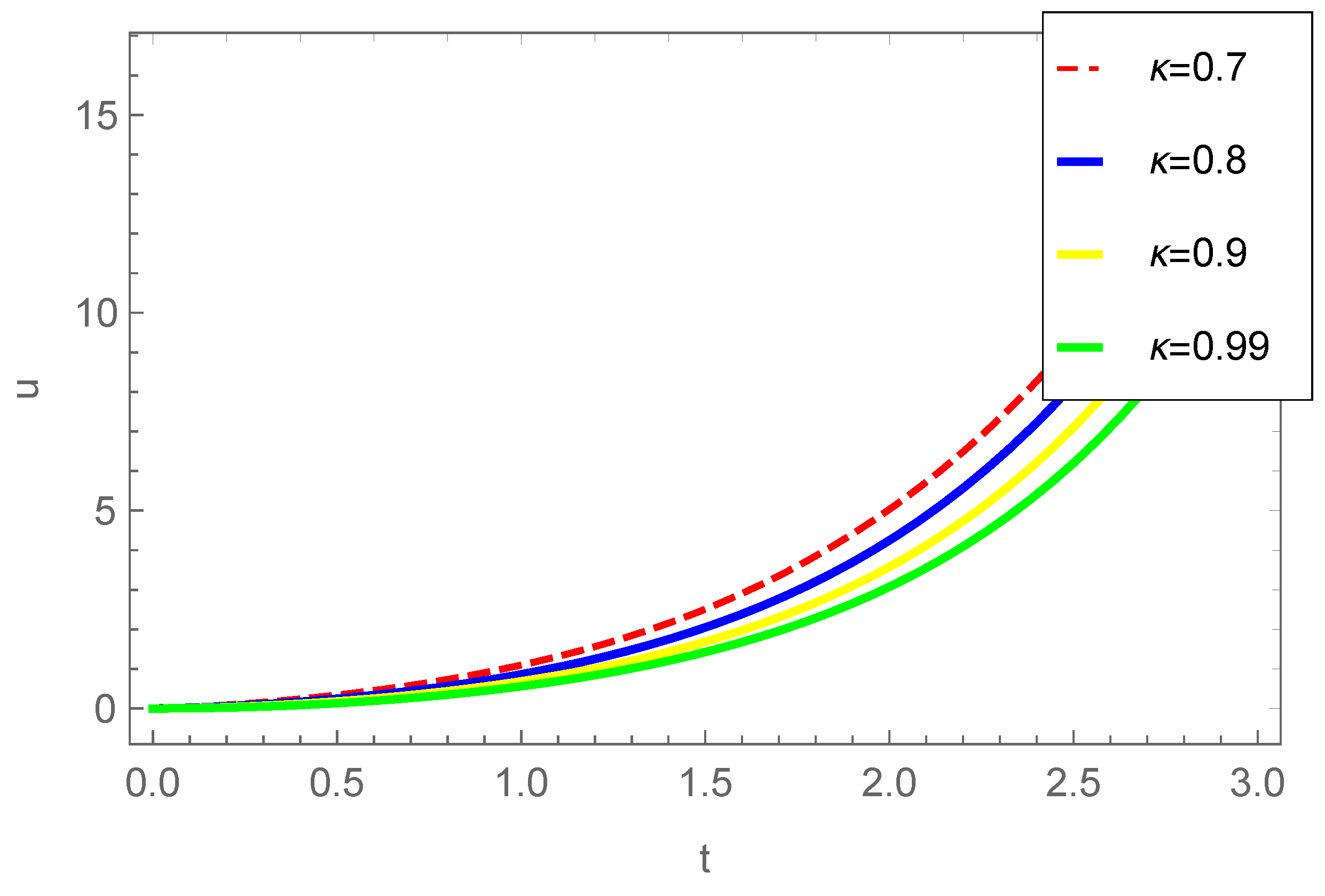
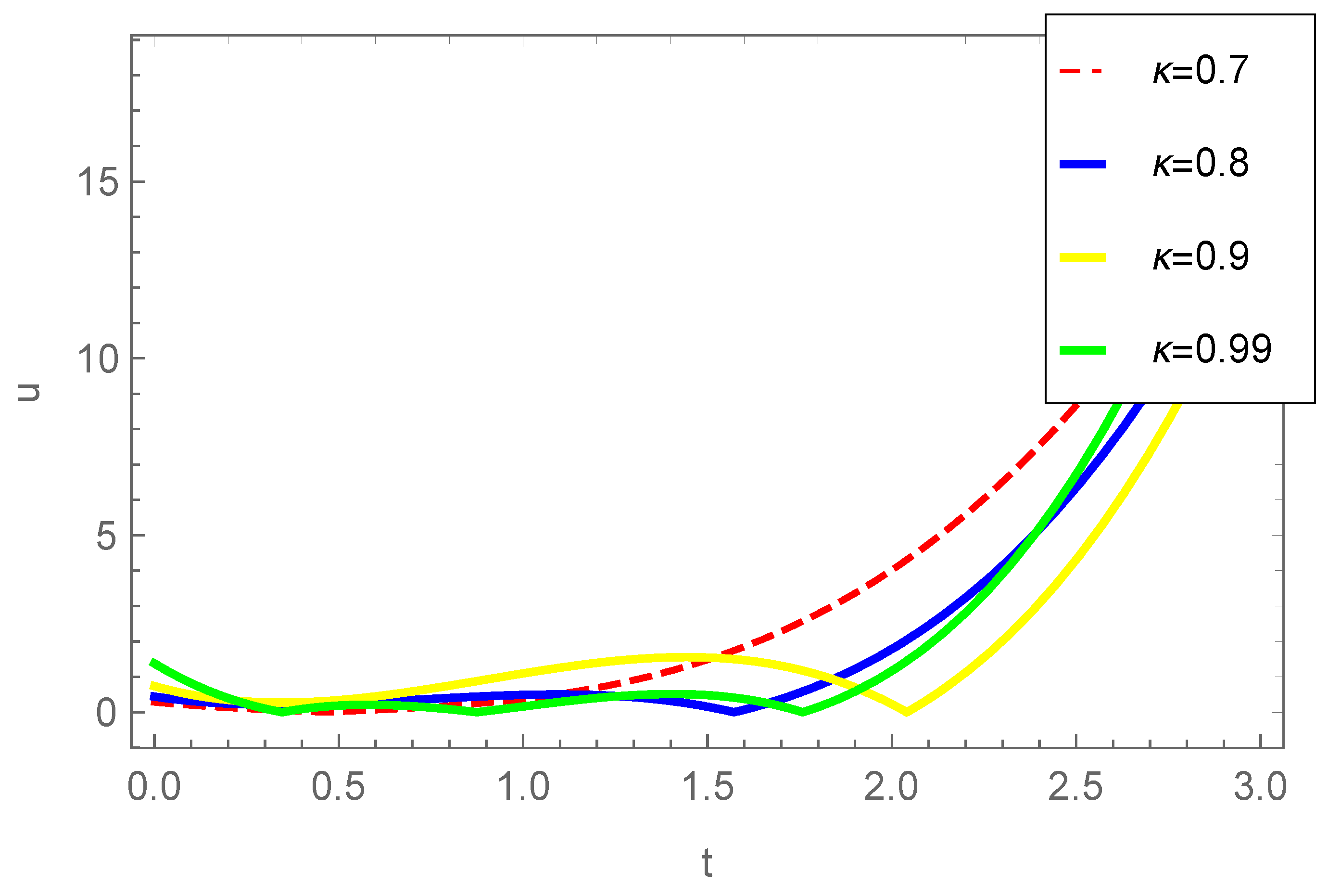
In this section, we examine the convergence of the solution to Equation (1).

Theorem 3. 

Let $u_n\left(t\right)$ and $u\left(t\right)$ be defined in Banach space, $B=\left(C\left[0,1\right],∥.∥\right)$, then the HPTM series ${\displaystyle \sum _{n=0}^{\infty }}{u}_n\left(t\right)$ converges to $u\left(t\right)$ of Equation (1) if there exists $\zeta \in \left(0,1\right)$ such that $∥u_{n+1}\left(t\right)∥\le \zeta \forall n\in N$.

Proof. 

Let us consider how the sequence of partial sums of series (18) is ${\left\{S_n\left(t\right)\right\}}_{n\ge 0}$ defined by

$$S_l\left(t\right)=\sum _{l=0}^{\infty }{u}_l\left(t\right).$$

(19)

Then

$$∥S_{n+1}\left(t\right)-S_n\left(t\right)∥=∥u_{n+1}\left(t\right)∥\le \zeta ∥u_n\left(t\right)∥\le {\zeta }^2∥u_{n-1}\left(t\right)∥\le \dots \le {\zeta }^{n+1}∥u_0\left(t\right)∥.$$

(20)

Now, first we have to show that $\left\{S_n\left(t\right)\right\}$ be a Cauchy sequence in Banach space $B=\left(C\left[0,1\right],∥.∥\right)$.

$$\begin{array}{c}∥S_q\left(t\right)-S_r\left(t\right)∥=∥S_q\left(t\right)-S_{q-1}\left(t\right)+S_{q-1}\left(t\right)-S_{q-2}\left(t\right)+...+S_{r+1}\left(t\right)-S_r\left(t\right)∥,\hfill \\ \\ \le ∥S_q\left(t\right)-S_{q-1}\left(t\right)∥+∥S_{q-1}\left(t\right)-S_{q-2}\left(t\right)∥+\dots ∥S_{r+1}\left(t\right)-S_r\left(t\right)∥,\hfill \\ \\ \le {\zeta }^q∥u_0\left(t\right)∥+{\zeta }^{q-1}∥u_0\left(t\right)∥+\dots +{\zeta }^{r+1}∥u_0\left(t\right)∥,\hfill \\ \\ \le {\zeta }^{r+1}\left(1+\zeta +{\zeta }^2+...+{\zeta }^q+...\right)∥u_0\left(t\right)∥,\hfill \\ \\ \le {\zeta }^{r+1}\left(\frac{1-{\zeta }^{q-r}}{1-\zeta }\right)∥u_0\left(t\right)∥.\hfill \end{array}$$

Since, $\zeta \in \left(0,1\right)$, so $1-{\zeta }^{q-r}>0$, then

$$∥S_q\left(t\right)-S_r\left(t\right)∥\le \frac{{\zeta }^{r+1}}{1-\zeta }∥u_0\left(t\right)∥.$$

(21)

Thus, ${∥S_q\left(t\right)-S_r\left(t\right)∥}_{q,r\to \infty }\to 0$ as $u_0$ is bounded.

This $\left\{S_n\left(t\right)\right\}$ is a Cauchy sequence in Banach space and hence convergent.

Therefore, there exists $u\in B$ such that

$$\sum _{l=0}^{\infty }{u}_l\left(t\right)=u\left(t\right).$$

We achieve the desired result. □

6. Special Cases

We have the normal generalized fractional operator. However, it may be reduced into three well-known fractional operators: Atangana-Baleanu-Caputo, Caputo, and Caputo-Fabrizio. To derive the results, we separately discuss the cases for generalized operators.

If we take n = 1, then (1) becomes

$$D_t^{2\kappa }u\left(t\right)+\delta E_{\beta }\left(u\right)=0,0<\kappa \le 1,0<t\le 1.$$

(22)

Moreover, consider the initial point u(0) = 0. This equation is known as a particular form of the generalized fractional Bratu equation.

We offer the solution to the generalized fractional Bratu equation in this section by using the process defined in Section 4.

Case 1. 

Consider generalized Bratu’s initial value problem for the Caputo fractional derivative,

$${ }^C{D}_t^{2\kappa }u\left(t\right)+\delta E_{\beta }\left(u\right)=0,$$

(23)

with u(0) = 0.

Applying Sumudu transform on (23),

$$S\left[{ }^C{D}_t^{2\kappa }u\left(t\right)\right]+\delta S\left[E_{\beta }\left(u\right)\right]=0,$$

or

$$s^{-2\kappa }\left\{S\left[u\left(t\right)\right]-u\left(0\right)\right\}=-\delta S\left[E_{\beta }\left(u\right)\right],$$

or

$$S\left[u\left(t\right)\right]=u\left(0\right)-\delta s^{2\kappa }S\left[E_{\beta }\left(u\right)\right].$$

Applying the inverse Sumudu transform,

$$u\left(t\right)=u\left(0\right)-\delta S^{-1}\left\{s^{2\kappa }S\left[E_{\beta }\left(u\right)\right]\right\}.$$

(24)

Now, using the homotopy perturbation transform method and expanding u(t) as $u\left(t\right)={\displaystyle \sum _{n=0}^{\infty }}{p}^n{u}_n\left(t\right)$, then (24) becomes

$$\sum _{n=0}^{\infty }{p}^n{u}_n\left(t\right)=u\left(0\right)-\delta p{S}^{-1}\left(s^{2\kappa }S\left[\sum _{n=0}^{\infty }{p}^n{H}_n\left(u\right)\right]\right).$$

(25)

Now, we have the Taylor’s series expansion of $E_{\beta }\left(u\right)$,

$$E_{\beta }\left(u\right)=\sum _{k=0}^{\infty }\frac{u^k}{\mathrm{\Gamma }(\beta k+1)}.$$

Now, comparing the coefficients in (25), we obtain

$$\begin{array}{c}{p}^0:u_0\left(t\right)=u\left(0\right),\hfill \\ \\ p^1:u_1\left(t\right)=-\delta S^{-1}\left(s^{2\kappa }S\left[H_0\left(u\right)\right]\right),\hfill \\ \\ p^2:u_2\left(t\right)=-\delta S^{-1}\left(s^{2\kappa }S\left[H_1\left(u\right)\right]\right),\hfill \\ \\ p^3:u_3\left(t\right)=-\delta S^{-1}\left(s^{2\kappa }S\left[H_2\left(u\right)\right]\right),\hfill \\ .\hfill \\ .\hfill \\ .\hfill \end{array}$$

Using u(0) = 0, we have

$$p^0:u_0\left(t\right)=0,$$

$$p^1:u_1\left(t\right)=-\delta S^{-1}\left(s^{2\kappa }S\left[1\right]\right)=-\delta \frac{t^{2\kappa }}{\mathrm{\Gamma }(2\kappa +1)},$$

$$p^2:u_2\left(t\right)=-\frac{\delta }{\mathrm{\Gamma }(\beta +1)}{S}^{-1}\left[s^{2\kappa }S\left(-\delta \frac{t^{2\kappa }}{\mathrm{\Gamma }(2\kappa +1)}\right)\right]=\frac{{\delta }^2}{\mathrm{\Gamma }(\beta +1)}\frac{t^{4\kappa }}{\mathrm{\Gamma }(4\kappa +1)},$$

$$\begin{array}{c}{p}^3:u_3\left(t\right)=-\delta S^{-1}\left(s^{2\kappa }S\left[\frac{u_2}{\mathrm{\Gamma }(\beta +1)}+\frac{{u_1}^2}{\mathrm{\Gamma }(2\beta +1)}\right]\right)\hfill \\ \\ ={\left(-\delta \right)}^3\left\{\frac{1}{{\left(\mathrm{\Gamma }(\beta +1)\right)}^2}+\frac{1}{\mathrm{\Gamma }(2\beta +1)}\frac{\mathrm{\Gamma }(4\kappa +1)}{{\left(\mathrm{\Gamma }(2\kappa +1)\right)}^2}\right\}\frac{t^{6\kappa }}{\mathrm{\Gamma }(6\kappa +1)},\hfill \end{array}$$

$$\begin{array}{c}.\hfill \\ .\hfill \\ .\hfill \end{array}$$

Now, the solution is given by (18),

$$\begin{array}{c}u\left(t\right)=(-\delta )\frac{t^{2\kappa }}{\mathrm{\Gamma }(2\kappa +1)}+\frac{{\left(-\delta \right)}^2}{\mathrm{\Gamma }(\beta +1)}\frac{t^{4\kappa }}{\mathrm{\Gamma }(4\kappa +1)}\hfill \\ \\ +{\left(-\delta \right)}^3\left\{\frac{1}{{\left(\mathrm{\Gamma }(\beta +1)\right)}^2}+\frac{1}{\mathrm{\Gamma }(2\beta +1)}\frac{\mathrm{\Gamma }(4\kappa +1)}{\mathrm{\Gamma }{(2\kappa +1)}^2}\right\}\frac{t^{6\kappa }}{\mathrm{\Gamma }(6\kappa +1)}+...\hfill \end{array}$$

Now to plot the results by considering δ = 1.0, β = 0.7 for different values of $\kappa$ as illustrated in Figure 1.

Remark 1. 

If we put $\beta =1$ in (23), then the equation becomes

$${ }^C{D}_t^{2\kappa }u\left(t\right)+\delta e^u=0,$$

and the solution is

$$u\left(t\right)=(-\delta )\frac{t^{2\kappa }}{\mathrm{\Gamma }(2\kappa +1)}+{(-\delta )}^2\frac{t^{4\kappa }}{\mathrm{\Gamma }(4\kappa +1)}+{\left(-\delta \right)}^3\left\{1+\frac{1}{2}\frac{\mathrm{\Gamma }(4\kappa +1)}{{\left(\mathrm{\Gamma }(2\kappa +1)\right)}^2}\right\}\frac{t^{6\kappa }}{\mathrm{\Gamma }(6\kappa +1)}+\dots$$

This solution for the fractional Bratu’s differential equation exactly matches the result of the analytical study of the fractional Bratu-type equation by Dubey et al. [49].

Now to plot the results by considering δ = 1.0, β = 1.0 for different values of, $\kappa$ as illustrated in Figure 2.

Case 2. 

Consider generalized Bratu’s initial value problem for the Caputo-Fabrizio derivative,

$${ }^{CF}{D}_t^{2\kappa }u\left(t\right)+\delta E_{\beta }\left(u\right)=0,$$

(26)

with u(0) = 0.

Applying Sumudu transform on (28),

$$S\left[{ }^{CF}{D}_t^{2\kappa }u\left(t\right)\right]+\delta S\left[E_{\beta }\left(u\right)\right]=0,$$

or

$$\frac{\Delta \left(2\kappa \right)}{\left(1-2\kappa +2\kappa s\right)}\left\{S\left[u\left(t\right)\right]-u\left(0\right)\right\}=-\delta S\left[E_{\beta }\left(u\right)\right],$$

or

$$S\left[u\left(t\right)\right]=u\left(0\right)-\frac{\delta \left(1-2\kappa +2\kappa s\right)}{\Delta \left(2\kappa \right)}S\left[E_{\beta }\left(u\right)\right].$$

Applying the inverse Sumudu transform,

$$u\left(t\right)=u\left(0\right)-\frac{\delta }{\Delta \left(2\kappa \right)}{S}^{-1}\left\{\left(1-2\kappa +2\kappa s\right)S\left[E_{\beta }\left(u\right)\right]\right\}.$$

(27)

Now, using the homotopy perturbation transform method and expanding u(t) as $u\left(t\right)={\displaystyle \sum _{n=0}^{\infty }}{p}^n{u}_n\left(t\right)$, we have

$$\sum _{n=0}^{\infty }{p}^n{u}_n\left(t\right)=u\left(0\right)-\frac{\delta p}{\Delta \left(2\kappa \right)}{S}^{-1}\left(\left(1-2\kappa +2\kappa s\right)S\left[\sum _{n=0}^{\infty }{p}^n{H}_n\left(u\right)\right]\right).$$

(28)

Using the Taylor’s series expansion of $E_{\beta }\left(u\right)$ and comparing the coefficients in (28), we obtain

$$\begin{array}{c}{p}^0:u_0\left(t\right)=u\left(0\right),\hfill \\ \\ p^1:u_1\left(t\right)=-\frac{\delta }{\Delta \left(2\kappa \right)}{S}^{-1}\left\{\left(1-2\kappa +2\kappa s\right)S\left[H_0\left(u\right)\right]\right\},\hfill \\ \\ p^2:u_2\left(t\right)=-\frac{\delta }{\Delta \left(2\kappa \right)}{S}^{-1}\left\{\left(1-2\kappa +2\kappa s\right)S\left[H_1\left(u\right)\right]\right\},\hfill \\ \\ p^3:u_3\left(t\right)=-\frac{\delta }{\Delta \left(2\kappa \right)}{S}^{-1}\left\{\left(1-2\kappa +2\kappa s\right)S\left[H_2\left(u\right)\right]\right\},\hfill \\ .\hfill \\ .\hfill \\ .\hfill \end{array}$$

Using u(0) = 0, we have

$$\begin{array}{ll}{p}^0:u_0\left(t\right)& =0,\\ p^1:u_1\left(t\right)& =-\frac{\delta }{\Delta \left(2\kappa \right)}\left\{(1-2\kappa )+2\kappa t\right\},\\ p^2:u_2\left(t\right)& ={\left(-\frac{\delta }{\Delta \left(2\kappa \right)}\right)}^2\frac{1}{\mathrm{\Gamma }(\beta +1)}\left\{{\left(1-2\kappa \right)}^2+4\kappa \left(1-2\kappa \right)t+2{\kappa }^2{t}^2\right\},\\ p^3:u_3\left(t\right)& ={\left(-\frac{\delta }{\Delta \left(2\kappa \right)}\right)}^3\left\{\left(\frac{1}{{\left(\mathrm{\Gamma }(\beta +1)\right)}^2}+\frac{1}{\mathrm{\Gamma }(2\beta +1)}\right)\left[{\left(1-2\kappa \right)}^3+6\kappa {\left(1-2\kappa \right)}^{2}t\right]\right.\\ & \left.+2\left(\frac{3}{{\left(\mathrm{\Gamma }(\beta +1)\right)}^2}+\frac{4}{\mathrm{\Gamma }(2\beta +1)}\right)\left(1-2\kappa \right){\kappa }^2{t}^2+\frac{8}{3!}\left(\frac{1}{{\left(\mathrm{\Gamma }(\beta +1)\right)}^2}+\frac{2}{\mathrm{\Gamma }(2\beta +1)}\right){\kappa }^3{t}^3\right\},\\ .\hfill & \\ .\hfill & \\ .\hfill & \end{array}$$

Now, the solution is given by (18),

$$\begin{array}{c}u\left(t\right)=\left(-\frac{\delta }{\Delta \left(2\kappa \right)}\right)\left\{(1-2\kappa )+2\kappa t\right\}+{\left(-\frac{\delta }{\Delta \left(2\kappa \right)}\right)}^2\frac{1}{\mathrm{\Gamma }(\beta +1)}\left\{{\left(1-2\kappa \right)}^2+4\kappa \left(1-2\kappa \right)t+2{\kappa }^2{t}^2\right\}\hfill \\ \hfill \\ +{\left(-\frac{\delta }{\Delta \left(2\kappa \right)}\right)}^3\left\{\left(\frac{1}{{\left(\mathrm{\Gamma }(\beta +1)\right)}^2}+\frac{1}{\mathrm{\Gamma }(2\beta +1)}\right)\left[{\left(1-2\kappa \right)}^3+6\kappa {\left(1-2\kappa \right)}^{2}t\right]\right.\hfill \\ \\ \left.+2\left(\frac{3}{{\left(\mathrm{\Gamma }(\beta +1)\right)}^2}+\frac{4}{\mathrm{\Gamma }(2\beta +1)}\right)\left(1-2\kappa \right){\kappa }^2{t}^2+\frac{8}{3!}\left(\frac{1}{{\left(\mathrm{\Gamma }(\beta +1)\right)}^2}+\frac{2}{\mathrm{\Gamma }(2\beta +1)}\right){\kappa }^3{t}^3\right\}+\dots \hfill \end{array}$$

Now to plot the results by considering δ = 1.0, β = 0.7 for different values of, $\kappa$ as illustrated in Figure 3.

Remark 2. 

If we put $\beta =1$ in (26), then the equation becomes

$${ }^{CF}{D}_t^{2\kappa }u\left(t\right)+\delta e^u=0,$$

and the solution is given by (18),

$$\begin{array}{c}u\left(t\right)=\left(-\frac{\delta }{\Delta \left(2\kappa \right)}\right)\left\{(1-2\kappa )+2\kappa t\right\}+{\left(-\frac{\delta }{\Delta \left(2\kappa \right)}\right)}^2\left\{{\left(1-2\kappa \right)}^2+4\kappa \left(1-2\kappa \right)t+2{\kappa }^2{t}^2\right\}\\ +{\left(-\frac{\delta }{\Delta \left(2\kappa \right)}\right)}^3\left\{\frac{3}{2}{\left(1-2\kappa \right)}^3+9\kappa {\left(1-2\kappa \right)}^{2}t+10\left(1-2\kappa \right){\kappa }^2{t}^2+\frac{8}{3}{\kappa }^3{t}^3\right\}+\dots \end{array}$$

Now to plot the results by considering δ = 1.0, β = 1.0 for different values of, κ as illustrated in Figure 4.

Case 3. 

Consider generalized Bratu’s initial value problem for the Atangana-Baleanu-Caputo derivative,

$${ }^{ABC}{D}_t^{2\kappa }u\left(t\right)+\delta E_{\beta }\left(u\right)=0,$$

(29)

with u(0) = 0.

Applying the Sumudu transform on (29),

$$S\left[{ }^{ABC}{D}_t^{2\kappa }u\left(t\right)\right]+\delta S\left[E_{\beta }\left(u\right)\right]=0,$$

or

$$\frac{\Delta \left(2\kappa \right)}{\left(1-2\kappa +2\kappa s^{2\kappa }\right)}\left\{S\left[u\left(t\right)\right]-u\left(0\right)\right\}=-\delta S\left[E_{\beta }\left(u\right)\right],$$

or

$$S\left[u\left(t\right)\right]=u\left(0\right)-\frac{\delta \left(1-2\kappa +2\kappa s^{2\kappa }\right)}{\Delta \left(2\kappa \right)}S\left[E_{\beta }\left(u\right)\right].$$

Applying the inverse Sumudu transform,

$$u\left(t\right)=u\left(0\right)-\frac{\delta }{\Delta \left(2\kappa \right)}{S}^{-1}\left\{\left(1-2\kappa +2\kappa s^{2\kappa }\right)S\left[E_{\beta }\left(u\right)\right]\right\}.$$

(30)

Now, using the homotopy perturbation transform method, we have

$$\sum _{n=0}^{\infty }{p}^n{u}_n\left(t\right)=u\left(0\right)-\frac{\delta p}{\Delta \left(2\kappa \right)}{S}^{-1}\left(\left(1-2\kappa +2\kappa s^{2\kappa }\right)S\left[\sum _{n=0}^{\infty }{p}^n{H}_n\left(u\right)\right]\right).$$

(31)

Using the Taylor’s series expansion of $E_{\beta }\left(u\right)$ and comparing the coefficients in (30), we obtain

$$\begin{array}{c}{p}^0:u_0\left(t\right)=u\left(0\right),\hfill \\ \\ p^1:u_1\left(t\right)=-\frac{\delta }{\Delta \left(2\kappa \right)}{S}^{-1}\left\{\left(1-2\kappa +2\kappa s^{2\kappa }\right)S\left[H_0\left(u\right)\right]\right\},\hfill \\ \\ p^2:u_2\left(t\right)=-\frac{\delta }{\Delta \left(2\kappa \right)}{S}^{-1}\left\{\left(1-2\kappa +2\kappa s^{2\kappa }\right)S\left[H_1\left(u\right)\right]\right\},\hfill \\ \\ p^3:u_3\left(t\right)=-\frac{\delta }{\Delta \left(2\kappa \right)}{S}^{-1}\left\{\left(1-2\kappa +2\kappa s^{2\kappa }\right)S\left[H_2\left(u\right)\right]\right\},\hfill \\ .\hfill \\ .\hfill \\ .\hfill \end{array}$$

Using u(0) = 0, we have

$$\begin{array}{c}{p}^0:u_0\left(t\right)=0,\hfill \\ \\ p^1:u_1\left(t\right)=-\frac{\delta }{\Delta \left(2\kappa \right)}\left\{(1-2\kappa )+2\kappa \frac{t^{2\kappa }}{\mathrm{\Gamma }(2\kappa +1)}\right\},\hfill \\ \\ p^2:u_2\left(t\right)={\left(-\frac{\delta }{\Delta \left(2\kappa \right)}\right)}^2\frac{1}{\mathrm{\Gamma }(\beta +1)}\left\{{\left(1-2\kappa \right)}^2+4\kappa \left(1-2\kappa \right)\frac{t^{2\kappa }}{\mathrm{\Gamma }(2\kappa +1)}+4{\kappa }^2\frac{t^{4\kappa }}{\mathrm{\Gamma }(4\kappa +1)}\right\},\hfill \\ .\hfill \\ .\hfill \\ .\hfill \end{array}$$

Now, the solution is given by (18),

$$\begin{array}{c}u\left(t\right)=\left(-\frac{\delta }{\Delta \left(2\kappa \right)}\right)\left\{(1-2\kappa )+2\kappa \frac{t^{2\kappa }}{\mathrm{\Gamma }(2\kappa +1)}\right\}+{\left(-\frac{\delta }{\Delta \left(2\kappa \right)}\right)}^2\frac{1}{\mathrm{\Gamma }(\beta +1)}\left\{{\left(1-2\kappa \right)}^2+\right.\hfill \\ \\ \left.4\kappa \left(1-2\kappa \right)\frac{t^{2\kappa }}{\mathrm{\Gamma }(2\kappa +1)}+4{\kappa }^2\frac{t^{4\kappa }}{\mathrm{\Gamma }(4\kappa +1)}\right\}+\dots \hfill \end{array}$$

Now to plot the results by considering δ = 1.0, β = 0.7 for different values of, κ as illustrated in Figure 5.

Remark 3. 

If we put $\beta =1$ in (29), then the equation becomes

$${ }^{ABC}{D}_t^{2\kappa }u\left(t\right)+\delta e^u=0,$$

and the solution is given by (18),

$$\begin{array}{c}u\left(t\right)=\left(-\frac{\delta }{\Delta \left(2\kappa \right)}\right)\left\{(1-2\kappa )+2\kappa \frac{t^{2\kappa }}{\mathrm{\Gamma }(2\kappa +1)}\right\}\hfill \\ \\ +\left(-\frac{\delta }{\Delta \left(2\kappa \right)}\right)\left\{{\left(1-2\kappa \right)}^2+\right.\left.4\kappa \left(1-2\kappa \right)\frac{t^{2\kappa }}{\mathrm{\Gamma }(2\kappa +1)}+4{\kappa }^2\frac{t^{4\kappa }}{\mathrm{\Gamma }(4\kappa +1)}\right\}+...\hfill \end{array}$$

Now to plot the results by considering δ = 1.0, β = 1.0 for different values of, κ as illustrated in Figure 6.

7. Conclusions

In this investigation, we have introduced and addressed the generalized nonlinear Bratu-type equation incorporating the generalized fractional derivatives operator. The solution is derived by applying an innovative analytical technique known as the homotopy perturbation transformation method. We have demonstrated the effectiveness of the generalized fractional derivatives operator and presented reduced results expressed in well-known fractional operators, including Caputo, Caputo-Fabrizio, and Atangana-Baleanu. Furthermore, various special cases of the generalized fractional Bratu’s equation have been identified and thoroughly examined. We also plot some numerical results to show the behavior of the obtained results.

References

1. Miller, K.S.; Ross, B. An Introduction to the Fractional Calculus and Fractional Differential Equations; A Wiley-Interscience Publication: New York, NY, USA, 1993; ISBN 0-471-58884-9. [Google Scholar]
2. Oldham, K.B.; Spanier, J. The Fractional Calculus-Theory and Applications of Differentiation and Integration to Arbitrary Order, 1st ed.; Mathematics in Science and Engineering: New York, NY, USA; London, UK, 1974; ISBN 978-012-525-550-9. [Google Scholar]
3. Kilbas, A.A.; Srivastava, H.M.; Trujillo, J.J. Theory and Applications of Fractional Differential Equations, 1st ed.; North-Holland Mathematics Studies: Amsterdam, The Netherlands, 2006; ISBN 978-0-444-51832-3. [Google Scholar]
4. Podlubny, I. Fractional Differential Equations—An Introduction to Fractional Derivatives, Fractional Differential Equations, to Methods of Their Solution and Some of Their Applications, 1st ed.; Mathematics in Science and Engineering: New York, NY, USA; London, UK, 1999; ISBN 978-0-12-558840-9. [Google Scholar]
5. Zhou, Y. Basic Theory of Fractional Differential Equations; World Scientific: Beijing, China, 2014; ISBN 978-981-4579-89-6. [Google Scholar]
6. Yang, X.J. Advanced Local Fractional Calculus and Its Applications; World Science Publisher: New York, NY, USA, 2012; ISBN 978-1-938576-01-0. [Google Scholar]
7. Yang, X.J.; Gao, F.; Srivastava, H.M. Exact travelling wave solutions for the local fractional two-dimensional Burger’s type equations. J. Comput. Appl. Math. 2017, 73, 203–210. [Google Scholar] [CrossRef]
8. Atangana, A. On the new fractional derivative and application to non-linear Fisher’s reaction-diffusion equation. Appl. Math. Comput. 2016, 273, 948–956. [Google Scholar] [CrossRef]
9. Saad, K.M.; Atangana, A.; Baleanu, D. New fractional derivatives with non-singular kernel applied to the Burgers equation. Chaos 2018, 28, 63–109. [Google Scholar] [CrossRef]
10. Daftardar-Gejji, V.; Jafari, H. Solving a multi-order fractional differential equation using adomian decomposition. Appl. Math. Comput. 2007, 189, 541–548. [Google Scholar] [CrossRef]
11. Wazwaz, A.M. A reliable modification of Adomian decomposition method. Appl. Math. Comput. 1999, 102, 77–86. [Google Scholar] [CrossRef]
12. Biazar, J.; Babolian, E.; Islam, R. Solution of the system of ordinary differential equations by Adomian decomposition method. Appl. Math. Comput. 2004, 147, 713–719. [Google Scholar] [CrossRef]
13. Hashim, I.; Abdulaziz, O.; Momani, S. Homotopy Analysis Method for Fractional IVPs. Commun. Nonlinear Sci. Numer. Simul. 2009, 14, 674–684. [Google Scholar] [CrossRef]
14. Liao, S. On the homotopy analysis method for nonlinear problems. Appl. Math. Comput. 2014, 147, 499–513. [Google Scholar] [CrossRef]
15. Liao, S. Notes on the homotopy analysis method: Some definitions and theorems. Commun. Nonlinear Sci. Numer. Simul. 2009, 14, 983–997. [Google Scholar] [CrossRef]
16. Odibat, Z.; Momani, S.; Erturk, V.S. Generalized differential transform method for solving a space- and time-fractional diffusion-wave equation. Phys. Lett. A 2007, 370, 379–387. [Google Scholar] [CrossRef]
17. Abdulaziz, O.; Hashim, I.; Momani, S. Solving systems of fractional differential equations by homotopy-perturbation method. Phys. Lett. A 2008, 372, 451–459. [Google Scholar] [CrossRef]
18. He, J.H. Homotopy perturbation method: A new nonlinear analytical technique. Appl. Math. Comput. 2003, 135, 73–79. [Google Scholar] [CrossRef]
19. Khan, Y. An effective modification of the laplace decomposition method for nonlinear equations. Int. J. Nonlinear Sci. Numer. Simul. 2009, 10, 1373–1376. [Google Scholar] [CrossRef]
20. Khan, Y. Homotopy perturbation transform method for nonlinear equations using He’s polynomials. Comput. Math. Appl. 2011, 61, 1963–1967. [Google Scholar] [CrossRef]
21. Khan, M.; Gondal, M.A.; Hussain, I.; Vanani, S.K. A new comparative study between homotopy analysis transform method and homotopy perturbation transform method on a semi infinite domain. Math. Comput. Model. 2012, 55, 1143–1150. [Google Scholar] [CrossRef]
22. Singh, J.; Kumar, D.; Swroop, R. Numerical solution of time- and space-fractional coupled Burger’s equations via homotopy algorithm. Alex. Eng. J. 2016, 55, 1753–1763. [Google Scholar] [CrossRef]
23. Mohamed, M.S.; Hamed, Y.S. Solving the convection–diffusion equation by means of the optimal q-homotopy analysis method (Oq-HAM). Results Phys. 2016, 6, 20–25. [Google Scholar] [CrossRef]
24. He, J.H. Homotopy perturbation technique. Comput. Methods Appl. Mech. Eng. 1999, 178, 257–262. [Google Scholar] [CrossRef]
25. He, J.H. Homotopy perturbation method for solving boundary value problems. Phys. Lett. A 2006, 350, 87–88. [Google Scholar] [CrossRef]
26. He, J.H. The homotopy perturbation method for nonlinear oscillators with discontinuities. Appl. Math. Comput. 2004, 151, 287–292. [Google Scholar] [CrossRef]
27. Caputo, M.; Fabrizio, M. A new definition of fractional derivative without singular kernel. Prog. Fract. Differ. Appl. 2015, 1, 73–85. [Google Scholar]
28. Gomez-Aguilar, J.F.; Atangana, A. New insight in fractional differentiation: Power, exponential decay and Mittag–Leffler laws and applications. Eur. Phys. J. Plus 2017, 132, 1–21. [Google Scholar] [CrossRef]
29. Gomez-Aguilar, J.F.; Atangana, A. Decolonisation of fractional calculus rules: Breaking commutativity and associativity to capture more natural phenomena. Eur. Phys. J. Plus 2018, 133, 166. [Google Scholar] [CrossRef]
30. Singh, J.; Kumar, D.; Swroop, R.; Kumar, S. An efficient computational approach for time-fractional Rosenau–Hyman equation. Neural Comput. Appl. 2017, 30, 3063–3070. [Google Scholar] [CrossRef]
31. Ascher, U.M.; Matheij, R.; Russell, R.D. Numerical Solution of Boundary Value Problems for Ordinary Differential Equations; Society for Industrial and Applied Mathematics: Philadelphia, PA, USA, 1995; ISBN 978-089-871-354-1. [Google Scholar]
32. Chandrasekhar, S. An Introduction to the Study of Stellar Structure; Dover: Chicago, IL, USA, 1957; ISBN 978-0-486-60413-8. [Google Scholar]
33. Ghazanfari, B.; Sepahvandzadeh, A. Homotopy perturbation method for solving fractional Bratu-type equation. J. Math. Model. 2015, 2, 143–155. [Google Scholar]
34. Ghazanfari, B.; Sepahvandzadeh, A. Solving fractional Bratu-type equations by modified variational iteration method. Selcuk. J. Appl. Math. 2014, 39, 23–29. [Google Scholar]
35. Ghazanfari, B.; Sepahvandzadeh, A. Adomian decomposition method for solving fractional Bratu-type equations. J. Math. Comput. Sci. 2014, 8, 236–244. [Google Scholar] [CrossRef]
36. Ghomanjani, F.; Shateyi, S. Numerical solution for fractional Bratu’s initial value problem. Open Phys. 2017, 15, 1045–1048. [Google Scholar] [CrossRef]
37. Demir, D.D.; Zeybek, A. The numerical solution of fractional Bratu-type differential equations. ITM Web Conf. 2017, 13, 1–11. [Google Scholar] [CrossRef]
38. Yi, M.; Sun, K.; Huang, J.; Wang, L. Numerical solution of fractional integrodifferential equations of bratu type by using CAS wavelets. J. Appl. Math. 2013, 2013, 801395. [Google Scholar] [CrossRef]
39. Kukushkin, M.V. Abstract Fractional Calculus for m-accretive Operators. Int. J. Appl. Math. 2021, 34, 1–41. [Google Scholar] [CrossRef]
40. Kukushkin, M.V. On Solvability of the Sonin–Abel Equation in the Weighted Lebesgue Space. Fractal Fract. 2021, 5, 77. [Google Scholar] [CrossRef]
41. Samko, S.G.; Kilbas, A.A.; Marichev, O.I. Fractional Integrals and Derivatives: Theory and Applications, 1st ed.; Gordon and Breach, Yverdon; CRC Press: Boca Raton, FL, USA, 1993; ISBN 2881248640. [Google Scholar]
42. Luchko, Y.; Yamamoto, M. General time-fractional diffusion equation: Some uniqueness and existence results for the initial boundary value problems. Fract. Calc. Appl. Anal. 2016, 19, 676–695. [Google Scholar] [CrossRef]
43. Oliveira, D.S.; Oliveira, E.C.D. On a Caputo-type fractional derivative. Adv. Pure Appl. Math. 2018, 10, 81–91. [Google Scholar] [CrossRef]
44. Qureshi, S.; Rangaig, N.A.; Baleanu, D. New Numerical Aspects of Caputo-Fabrizio Fractional Derivative Operator. Mathematics 2019, 7, 374. [Google Scholar] [CrossRef]
45. Yadav, S.; Pandey, R.K.; Shukla, A.K. Numerical approximations of Atangana–Baleanu Caputo derivative and its application. Chaos Solitons Fractals 2019, 118, 58–64. [Google Scholar] [CrossRef]
46. Demiray, S.T.; Bulut, H.; Belgacem, F.B.M. Sumudu Transform Method for Analytical Solutions of Fractional Type Ordinary Differential Equations. Math. Probl. Eng. 2014, 2015, 131690. [Google Scholar] [CrossRef]
47. Atangana, A.; Akgul, A. Can transfer function and Bode diagram be obtained from Sumudu transform. Alex. Eng. J. 2019, 59, 1971–1984. [Google Scholar] [CrossRef]
48. Bodkhe, D.S.; Panchal, S.K. On Sumudu Transform Of Fractional Derivatives and Its Applications to Fractional Differential Equations. Asian J. Math. Comput. 2016, 11, 69–77. [Google Scholar]
49. Dubey, V.P.; Kumar, R.; Kumar, D. Analytical study of fractional Bratu-type equation arising in electro-spun organic nanofibers elaboration. Phys. A 2019, 521, 762–772. [Google Scholar] [CrossRef]
Figure 1. Change in u for Case 1 with respect to time, for different values of κ .
Axioms 13 00133 g001
Figure 2. Change in u for remark of Case 1 with respect to time, for different values of κ .
Axioms 13 00133 g002
Figure 3. Change in u for Case 2 with respect to time, for different values of κ .
Axioms 13 00133 g003
Figure 4. Change in u for remark of Case 2 with respect to time, for different values of κ .
Axioms 13 00133 g004
Figure 5. Change in u for Case 3 with respect to time, for different values of κ .
Axioms 13 00133 g005
Figure 6. Change in u for remark of Case 3 with respect to time, for different values of κ .
Axioms 13 00133 g006
Disclaimer/Publisher’s Note: The statements, opinions and data contained in all publications are solely those of the individual author(s) and contributor(s) and not of MDPI and/or the editor(s). MDPI and/or the editor(s) disclaim responsibility for any injury to people or property resulting from any ideas, methods, instructions or products referred to in the content.