An Algorithm Based on Compute Unified Device Architecture for Estimating Covering Functionals of Convex Bodies

Abstract

In Chuanming Zong’s program to attack Hadwiger’s covering conjecture, which is a longstanding open problem from Convex and Discrete Geometry, it is essential to estimate covering functionals of convex bodies effectively. Recently, He et al. and Yu et al. provided two deterministic global optimization algorithms having high computational complexity for this purpose. Since satisfactory estimations of covering functionals will be sufficient in Zong’s program, we propose a stochastic global optimization algorithm based on CUDA and provide an error estimation for the algorithm. The accuracy of our algorithm is tested by comparing numerical and exact values of covering functionals of convex bodies including the Euclidean unit disc, the three-dimensional Euclidean unit ball, the regular tetrahedron, and the regular octahedron. We also present estimations of covering functionals for the regular dodecahedron and the regular icosahedron.

1. Introduction

A compact convex subset K of ${\mathbb{R}}^n$ having interior points is called a convex body, whose boundary and interior are denoted by $bdK$ and $intK$, respectively. Let ${\mathcal{K}}^n$ be the set of convex bodies in ${\mathbb{R}}^n$. For each $K\in {\mathcal{K}}^n$, let $c\left(K\right)$ be the least number of translates of $intK$ necessary to cover K. Regarding the least upper bound of $c\left(K\right)$ in ${\mathcal{K}}^n$, there is a long-standing conjecture:

Conjecture 1

(Hadwiger’s covering conjecture). For each $K\in {\mathcal{K}}^n$, we have

$$c\left(K\right)\le 2^n;$$

the equality holds if and only if K is a parallelotope.

Classical results related to this conjecture can be found in [1,2]. While extensive research has been conducted (see e.g., refs. [3,4,5,6,7]), Conjecture 1 has only been conclusively resolved when $n=2$.

For each $p\in {\mathbb{Z}}^{+}$, set $\left[p\right]=\left\{i\in {\mathbb{Z}}^{+}\mid 1\le i\le p\right\}$.

Let $K\in {\mathcal{K}}^n$. A set having the form $\lambda K+x$, where $\lambda \in (0,1)$ and $x\in {\mathbb{R}}^n$, is called a smaller homothetic copy of K. According to Theorem 34.3 in [1], $c\left(K\right)$ equals the least number of smaller homothetic copies of K required to cover K. Clearly, $c\left(K\right)\le p$ for some $p\in {\mathbb{Z}}^{+}$ if and only if ${\Gamma }_p\left(K\right)<1$, where

$${\Gamma }_p\left(K\right):=min\left\{\gamma >0\mid \exists \left\{x_i\mid i\in \left[p\right]\right\}\subseteq {\mathbb{R}}^n\mathrm{s}.\mathrm{t}.K\subseteq \bigcup _{i\in \left[p\right]}(\gamma K+x_i)\right\}.$$

For each $p\in {\mathbb{Z}}^{+}$, the map

$$\begin{array}{cc}\hfill {\Gamma }_p(·):{\mathcal{K}}^n& \to [0,1]\hfill \\ \hfill K& \mapsto {\Gamma }_p\left(K\right)\hfill \end{array}$$

is an affine invariant and is called the covering functional with respect to p. Let $K\in {\mathcal{K}}^n$ and $p\in {\mathbb{Z}}^{+}$. A set C of p points satisfying

$$K\subseteq {\Gamma }_p\left(K\right)K+C,$$

is called a p-optimal configuration of K.

In [8], Chuanming Zong proposed the first program based on computers to tackle Conjecture 1 via estimating covering functionals. Two different algorithms have been designed for this purpose. The first one is introduced by Chan He et al. (cf. [9]) based on the geometric branch-and-bound method (cf. [10]). The algorithm is implemented in two parts. The first part uses geometric branch-and-bound methods to estimate $\Gamma (K,C)$, where

$$\Gamma (K,C)=min\left\{\gamma >0\mid K\subseteq C+\gamma K\right\}.$$

The second part also uses geometric branch-and-bound methods to estimate ${\Gamma }_p\left(K\right)$. When $n\ge 3$, computing $\Gamma (K,C)$ and ${\Gamma }_p\left(K\right)$ in this way exhibits a significantly high computational complexity. The other is introduced by Man Yu et al. (cf. [11]) based on the relaxation algorithm. Let $S\subseteq K$ be a discretization of K, $P_K$ be a set containing a p-optimal configuration of K, and $V\subseteq P_K$. They transformed the problem of covering S by smaller homothetic copies of K into a vertex p-center problem, and showed that the solution of the corresponding vertex p-center problem is a good approximation of ${\Gamma }_p\left(K\right)$ by proving

$${\Gamma }_p\left(S\right)-{\epsilon }_1\le {\Gamma }_p\left(K\right)\le {\Gamma }_p\left(S\right)+{\epsilon }_2,$$

where

$${\Gamma }_p\left(S\right)=min\left\{\gamma >0\mid \exists \left\{x_i\mid i\in \left[p\right]\right\}\subseteq {\mathbb{R}}^n\mathrm{s}.\mathrm{t}.S\subseteq \bigcup _{i\in \left[p\right]}(\gamma K+x_i)\right\},$$

and ${\epsilon }_1$ and ${\epsilon }_2$ are two positive numbers satisfying

$$K\subseteq S+{\epsilon }_{1}K\mathrm{and}{P}_K\subseteq V+{\epsilon }_{2}K.$$

Clearly, finer discretizations of K are required to obtain more accurate estimates of ${\Gamma }_p\left(K\right)$, which will lead to higher computational complexity.

In this paper, we propose an algorithm utilizes Compute Unified Device Architecture (CUDA) and stochastic global optimization methods to accelerate the process of estimating ${\Gamma }_p\left(K\right)$. CUDA is a parallel computing platform, particularly well-suited for handling large-scale computational tasks by performing many computations in parallel (cf. [12]). When discretizing convex bodies, CUDA provides a natural discretization method and enables parallel computation for all discretized points, thereby accelerating the execution of algorithms. As show in Section 2, when calculating $\Gamma (S,C)$ for some $C\subseteq {\mathbb{R}}^n$, we need to obtain the maximum dissimilarity between a point in S and its closest point in C. The reduction technique provided by CUDA, which typically involves performing a specific operation on all elements in an array (summation, finding the maximum, finding the minimum, etc., cf. [13]), enables the efficient computation of $\Gamma (S,C)$. When facing large-scale optimization problems, stochastic algorithms have the capability to produce high-quality solutions in a short amount of time.

In Section 2, the problem of estimating ${\Gamma }_p\left(K\right)$ is transformed into a minimization optimization problem, and an error estimation is provided. Using ideas mentioned in [9], an algorithm based on CUDA for ${\Gamma }_p\left(S\right)$ is designed in Section 3. Results of computational experiments showing the effectiveness of our algorithm are presented in Section 4.

2. Covering Functional and Error Estimation

As in [9], we put $Q_n={[-1,1]}^n$. For each $K\in {\mathcal{K}}^n$, let

$$\alpha \left(K\right)=max\left\{\alpha >0\mid \exists T\in {\mathcal{A}}^n\mathrm{s}.\mathrm{t}.\alpha Q_n\subseteq T\left(K\right)\subseteq Q_n\right\},$$

where ${\mathcal{A}}^n$ is the set of all non-singular affine transformations on ${\mathbb{R}}^n$. We can apply an appropriate affine transformation, if necessary, to ensure that

$$\alpha \left(K\right)Q_n\subseteq K\subseteq Q_n.$$

Remark 1.

In general, it is not easy to calculate $\alpha \left(K\right)$. If K is symmetric about the origin, then $1\alpha \left(K\right)$ is the Banach–Mazur distance between K and $Q_n$. By Proposition 37.6 in [14], when K is the n-dimensional Euclidean unit ball $B_2^n$, $1\alpha \left(K\right)=\sqrt{n}$. For our purpose, it will be sufficient to choose an α, as large as possible, such that $\alpha Q_n\subseteq K\subseteq Q_n$.

Definition 1

(cf. [11]). Let $K\in {\mathcal{K}}^n$. For k, $c\in {\mathbb{R}}^n$, the number

$$d(k,c)=min\left\{\gamma \ge 0\mid k\in \gamma K+c\right\}.$$

(1)

is called the dissimilarity of k and c.

If $K=B_2^n$, the dissimilarity between any two points is precisely the Euclidean distance between these two points. In general, the dissimilarity is not symmetric. If K is an n-dimensional convex polytope, the dissimilarity between any two points can be computed by Lemma 1.

Lemma 1.

Let $K\in {\mathcal{K}}^n$ be an n-dimensional convex polytope with $o\in intK$ determined by

$$K=\left\{x\in {\mathbb{R}}^n\mid Ax\le B\right\},$$

(2)

where A is an m-by-n matrix and B is an m-dimensional column vector whose elements are all 1. For any $u,c\in {\mathbb{R}}^n$, we have

$$d(u,c)=\underset{1\le i\le m}{max}{p}_i,$$

(3)

where ${\left(p_i\right)}_{m\times 1}=A(u-c)$.

Proof. 

Since K is bounded, $\underset{1\le i\le m}{max}{p}_i\ge 0$. Let

$${\gamma }_0=min\left\{\gamma \ge 0\mid u\in c+\gamma K\right\}.$$

For positive $\gamma$, we have

$$u-c\in \gamma K\iff \frac{1}{\gamma }(u-c)\in K\iff \frac{1}{\gamma }A(u-c)\le B\iff A(u-c)\le \gamma B.$$

Since $B={(1,1\dots ,1)}^T$, we have $\underset{1\le i\le m}{max}{p}_i\le \gamma$, which implies that

$$\underset{1\le i\le m}{max}{p}_i\le {\gamma }_0=d(u,c).$$

(4)

Since $p_i\le \underset{1\le j\le m}{max}{p}_j,\forall i\in \left[m\right]$, we have $A(u-c)\le \left(\underset{1\le i\le m}{max}{p}_i\right)B$. Thus,

$$u-c\in \left(\underset{1\le i\le m}{max}{p}_i\right)K,$$

which implies that

$$\underset{1\le i\le m}{max}{p}_i\ge {\gamma }_0=d(u,c).$$

(5)

The desired equality (3) follows from (4) and (5).    □

Remark 2.

Clearly, each convex polytope K containing the origin 0 in its interior can be represented as (2).

Let $i\ge 2$ and $j\in \left[n\right]$ be two integers. We denote by $p_j\left(x\right)$ the j-th coordinate of a point $x\in {\mathbb{R}}^n$ and

$$S_i=\left\{({\gamma }_1,\cdots ,{\gamma }_n)\in {\mathbb{R}}^n\mid {\gamma }_j\in \left\{-1+\frac{2k}{i-1}\mid k\in [i-1]\cup 0\right\},\forall j\in \left[n\right]\right\}.$$

Lemma 2.

$Q_n\subseteq S_i+\frac{1}{i-1}{Q}_n$.

Proof. 

Suppose that $x=({\beta }_1,\cdots ,{\beta }_n)\in Q_n$. Let $y\in {\mathbb{R}}^n$ be the point satisfying

$$p_j\left(y\right)=\left\{\begin{array}{cc}\frac{\lfloor {\beta }_j(i-1)\rfloor }{i-1},\hfill & \lfloor {\beta }_j(i-1)\rfloor +i-1\mathrm{is}\mathrm{even},\hfill \\ \frac{\lfloor {\beta }_j(i-1)\rfloor +1}{i-1},\hfill & \lfloor {\beta }_j(i-1)\rfloor +i-1\mathrm{is}\mathrm{odd},\hfill \end{array}\right.\forall j\in \left[n\right].$$

Then, $y\in S_i$. Let $j\in \left[n\right]$. If $\lfloor {\beta }_j(i-1)\rfloor +i-1$ is even, then

$$|{\beta }_j-p_j\left(y\right)|=\frac{{\beta }_j(i-1)-\lfloor {\beta }_j(i-1)\rfloor }{i-1}\le \frac{1}{i-1}.$$

Otherwise, we have

$$|{\beta }_j-p_j\left(y\right)|=\frac{|{\beta }_j(i-1)-\lfloor {\beta }_j(i-1)\rfloor -1|}{i-1}\le \frac{1}{i-1}.$$

It follows that ${||x-y||}_{\infty }\le \frac{1}{i-1}$. Therefore,

$$x\in y+\frac{1}{i-1}{Q}_n\subseteq S_i+\frac{1}{i-1}{Q}_n.$$

   □

Theorem 1.

Let $\alpha >0$ and $i\ge 2$ be an integer. If $K\in {\mathcal{K}}^n$ satisfies $\alpha Q_n\subseteq K\subseteq Q_n$, then

$$K\subseteq (S_i\cap \left(\frac{1+\alpha (i-1)}{\alpha (i-1)}K\right))+\frac{1}{i-1}{Q}_n.$$

Proof. 

By Lemma 2, we have

$$Q_n\subseteq S_i+\frac{1}{i-1}{Q}_n.$$

It follows that

$$K\subseteq (S_i+\frac{1}{i-1}{Q}_n)\cap K.$$

Let $x\in K$. There exists a point $p\in S_i$ such that

$$x\in p+\frac{1}{i-1}{Q}_n.$$

Thus,

$$p\in x-\frac{1}{i-1}{Q}_n\subseteq K+\frac{1}{i-1}{Q}_n\subseteq K+\frac{1}{\alpha (i-1)}K=\frac{1+\alpha (i-1)}{\alpha (i-1)}K.$$

Therefore, we have

$$x\in (S_i\cap \left(\frac{1+\alpha (i-1)}{\alpha (i-1)}K\right))+\frac{1}{i-1}{Q}_n.$$

   □

Let $\alpha >0$, $i\ge 2$ be an integer, K be a convex body satisfying $\alpha Q_n\subseteq K\subseteq Q_n$,

$$S=S_i\cap \left(\frac{1+\alpha (i-1)}{\alpha (i-1)}K\right),$$

(6)

and $C\subseteq {\mathbb{R}}^n$. Put

$$\Gamma (S,C)=inf\left\{\gamma >0\mid S\subseteq C+\gamma K\right\},$$

and

$${\Gamma }_p\left(S\right)=min\left\{\Gamma (S,C)\mid C\mathrm{contains}\mathrm{at}\mathrm{most}p\mathrm{points}\right\}.$$

Proposition 1.

Let K, α, i, S be as above, $p\in {\mathbb{Z}}^{+}$. Then,

$${\Gamma }_p\left(K\right)\le {\Gamma }_p\left(S\right)+\frac{1}{\alpha (i-1)}.$$

(7)

Proof. 

By Theorem 1, we have

$$K\subseteq S+\frac{1}{i-1}{Q}_n\subseteq S+\frac{1}{\alpha (i-1)}K.$$

Let $C^{\prime }$ be a p-element subset of ${\mathbb{R}}^n$ such that $S\subseteq C^{\prime }+{\Gamma }_p\left(S\right)K$. We have

$$K\subseteq S+\frac{1}{\alpha (i-1)}K\subseteq C^{\prime }+{\Gamma }_p\left(S\right)K+\frac{1}{\alpha (i-1)}K,$$

which completes the proof.    □

3. An Algorithm Based on CUDA for ${\Gamma }_{\mathbf{p}}\left(\mathbf{S}\right)$

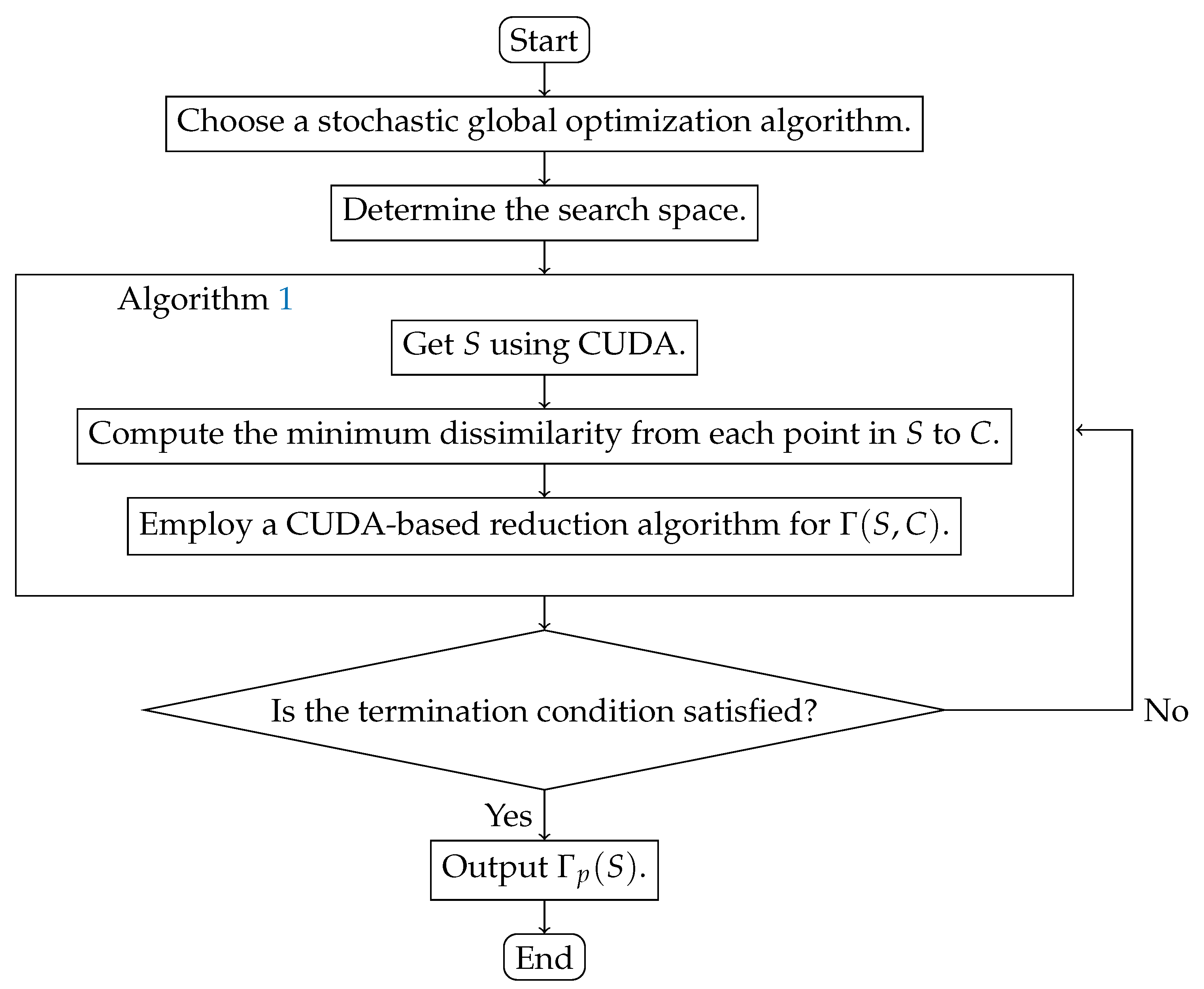
Let $K\in {\mathcal{K}}^n$, $p\in {\mathbb{Z}}^{+}$, and C be a set of p points. First, we use CUDA to obtain S defined by (6) and compute the minimum dissimilarity from each point in S to C. Then, we employ a CUDA-based reduction algorithm to obtain $\Gamma (S,C)$. Finally, we use different stochastic global optimization algorithms to estimate ${\Gamma }_p\left(S\right)$ and select an appropriate optimization algorithm through comparison. Figure 1 shows the overall framework of the algorithm.

3.1. An Algorithm Based on CUDA for $\Gamma (S,C)$

CUDA organizes threads into a hierarchical structure consisting of grids, blocks, and threads. The grid is the highest-level organization of threads in CUDA, and a grid represents a collection of blocks. A block, identified by a unique block index within its grid, is a group of threads that can cooperate with each other and share data using shared memory. Threads are organized within blocks, and each thread is identified by a unique thread index within its block. The number of blocks and threads per block can be specified when launching a CUDA kernel. The grid and block dimensions can be one-dimensional, two-dimensional, or three-dimensional, depending on the problem to address. For more information about CUDA, we refer to [15,16,17,18].

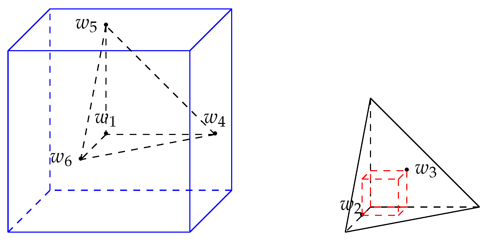
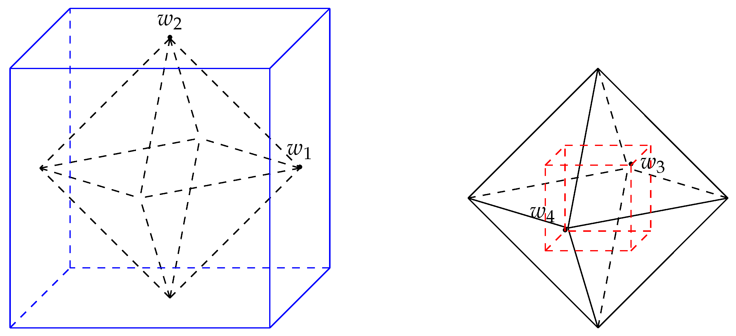
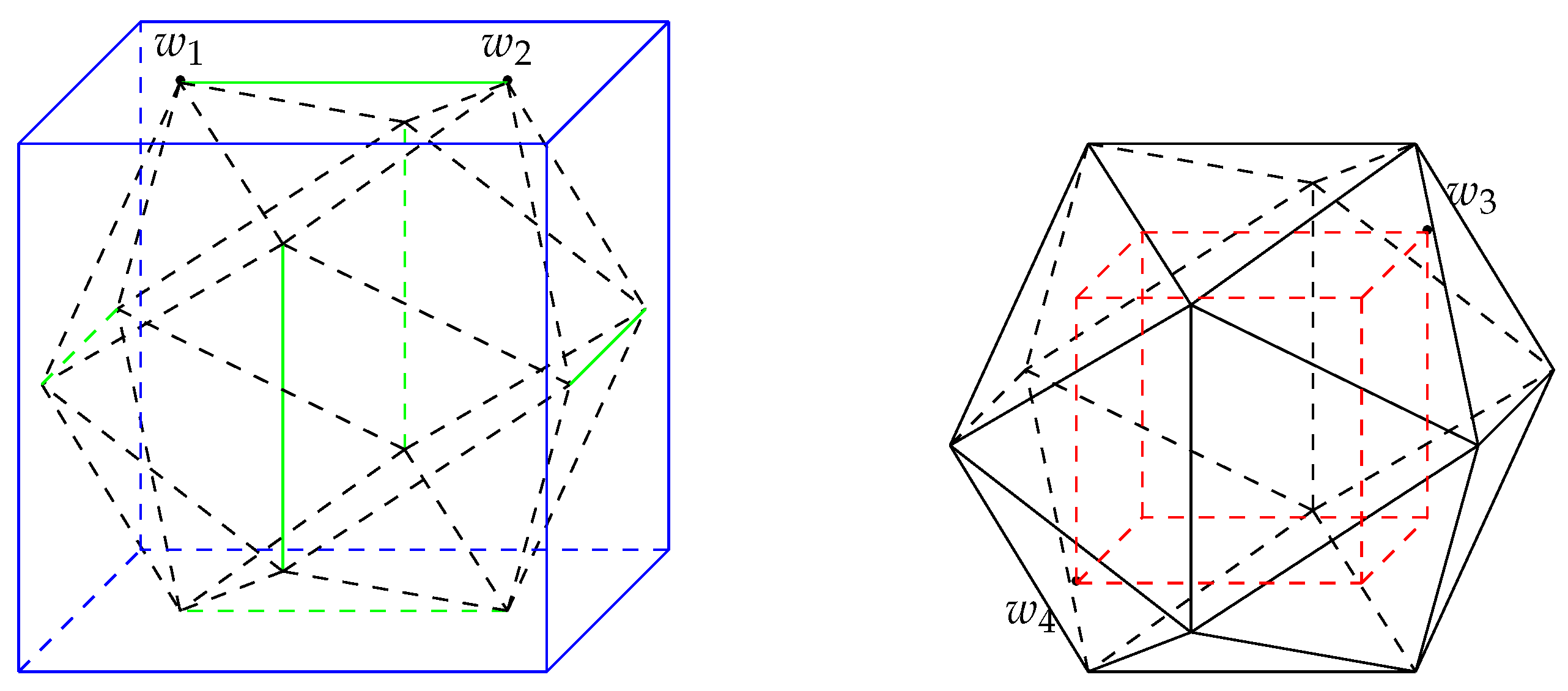
The organization of threads within blocks and grids provides a natural way to discretize $Q_3$. First, we discretize $[-1,1]\times [-1,1]\times 0$ into a set P of (gridDim.x)$\times$(gridDim.y) points. Each point p in P corresponds to a block $B_p$ in CUDA. And $B_p$ contains a collection of blockDim.x threads, each one of which corresponds to a point in $p+0\times 0\times [-1,1]$. See Figure 2, where gridDim.x, girdDim.y, and blockDim.x are set to be 5.

Let T be the set of all threads invoked by CUDA. Then, the cardinality of T is

$$\mathrm{gridDim}.\mathrm{x}\times \mathrm{gridDim}.\mathrm{y}\times \mathrm{blockDim}.\mathrm{x}.$$

For $i\in [\mathrm{gridDim}.\mathrm{x}-1]\cup \left\{0\right\}$, $j\in [\mathrm{gridDim}.\mathrm{y}-1]\cup \left\{0\right\}$, and $k\in [\mathrm{blockDim}.\mathrm{x}-1]\cup \left\{0\right\}$, there is a thread $t:=t(i,j,k)\in T$ indexed by

$$(j\times \mathrm{gridDim}.\mathrm{x}+i)\times \mathrm{blockDim}.\mathrm{x}+k,$$

which corresponds to the point

$$p_t=(-1+\frac{2i}{\mathrm{gridDim}.\mathrm{x}-1},-1+\frac{2j}{\mathrm{gridDim}.\mathrm{y}-1},-1+\frac{2k}{\mathrm{blockDim}.\mathrm{x}-1})\in Q_3.$$

Put

$$S=\left\{t\in T\mid p_t\in (1+\frac{1}{\alpha (\mathrm{gridDim}.\mathrm{x}-1)})K\right\},$$

where $\alpha$ is a positive number satisfying $\alpha Q_3\subseteq K\subseteq Q_3$. For each $t\in S$, denote by $d(p_t,C)$ the minimum dissimilarity from point $p_t$ to C, i.e.,

$$d(p_t,C)=min\left\{d(p_t,c)\mid c\in C\right\}.$$

If $t\notin S$, we set $d(p_t,C)=0$. The CUDA thread corresponding to $t\in T$ computes $d(p_t,C)$. Then, a CUDA-based reduction algorithm will be invoked to obtain ${max}_{t\in T}d(p_t,C)$.

The idea of the reduction algorithm based on CUDA is to divide the original data into multiple blocks, and then perform a local reduction operation on each block to obtain the local reduction result, and, finally, a global reduction operation is performed on the local reduction results to obtain the final reduction result (cf. [19]).

Algorithm 1 with parameters K, C, p, blockDim.x, gridDim.x, gridDim.y, and $\alpha$ calculates $\Gamma (S,C)$. It is more efficient than the geometric branch-and-bound approach proposed in [9]. For example, take $K=B_2^3$, $p=6$,

$$\begin{array}{cc}\hfill C_1=\{& (0.125,0.125,0.125),(-0.125,-0.125,-0.125),(0.25,0.25,0.25),\hfill \\ \hfill & (-0.25,-0.25,-0.25),(0.5,0.5,0.5),(-0.5,-0.5,-0.5),\hfill \\ \hfill & (0.0375,0.0375,0.0375),(-0.0375,-0.0375,-0.0375)\},\mathrm{and}\hfill \\ \hfill C_2=\{& (0,0.57,-0.38),(0.074,-0.185,0.618),(-0.05,-0.66,0.13),\hfill \\ \hfill & (0.32,-0.25,-0.58),(-0.52,-0.15,-0.38),(-0.587,0.123,0.22),\hfill \\ \hfill & (0.662,-0.024,0.013),(0.136,0.589,0.319)\}.\hfill \end{array}$$

Algorithm 1 An algorithm based on CUDA to compute $\Gamma (S,C)$

Require:  a convex body K, a set C of p points in ${\mathbb{R}}^n$, a positive number $\alpha$, blockDim.x, gridDim.x and gridDim.y Ensure:  $max$ as an estimation of $\Gamma (S,C)$  1: Host and device allocate memory, initialize and copy host data to device  2: $bid\leftarrow \mathrm{blockIdx}.\mathrm{y}\ast \mathrm{gridDim}.\mathrm{x}+\mathrm{blockIdx}.\mathrm{x}$  3: $t\leftarrow bid\ast \mathrm{blockDim}.\mathrm{x}+\mathrm{threadIdx}.\mathrm{x}$  4: $x\left[t\right]\leftarrow -1+2/(\mathrm{gridDim}.\mathrm{x}-1)\ast \mathrm{blockIdx}.\mathrm{x}$  5: $y\left[t\right]\leftarrow -1+2/(\mathrm{gridDim}.\mathrm{y}-1)\ast \mathrm{blockIdx}.\mathrm{y}$  6: $z\left[t\right]\leftarrow -1+2/(\mathrm{blockDim}.\mathrm{x}-1)\ast \mathrm{threadIdx}.\mathrm{x}$  7: $p\left[t\right]\leftarrow \left(x\right[id],y[id],z[id\left]\right)$  8: if $(p\left[t\right]\in (1+\frac{1}{\alpha (\mathrm{gridDim}.\mathrm{x}-1)})K$then:  9:      Calculate $d\left(p\right[t],C)$ by Lemma 1 10:     $P\left[t\right]\leftarrow d\left(p\right[t],C)$ 11: else 12:     $P\left[t\right]\leftarrow 0$ 13: end if 14: $sData\left[\mathrm{threadIdx}.\mathrm{x}\right]\leftarrow P\left[t\right]$ 15: Using the reduction algorithm to find the maximum value 16: $Dd\left[\mathrm{blockIdx}.\mathrm{x}\right]\leftarrow sData\left[0\right]$ 17: Copy the final reduction result to the host, $D\left[0\right]\leftarrow Dd\left[\mathrm{blockIdx}.\mathrm{x}\right]$ 18: $max\leftarrow D\left[0\right]$ 19: return  $max$

Algorithm 1 yields good estimations of ${\Gamma }_p(S,C_1)$ and ${\Gamma }_p(S,C_2)$ much faster, as seen in

Table 1. Comparison of results between the algorithm based on CUDA and the geometric branch-and-bound approach.

Algorithm	Algorithm 1	The Geometric Branch-and-Bound Approach
accuracy	$\frac{\sqrt{3}}{1023}$	0.0001
$\Gamma (S,C_1)$	1.002750…	1.002089…
Time	42.258720 ms	32.594993 s
$\Gamma (S,C_2)$	0.748103…	0.748099…
Time	42.232449 ms	0.303316 s

. Both algorithms run on a computer equipped with an AMD Ryzen 9 3900X 12-core processor and the NVIDIA A4000 graphics processor. For Algorithm 1, we take $\mathrm{gridDim}.\mathrm{x}=\mathrm{gridDim}.\mathrm{y}=\mathrm{blockDim}.\mathrm{x}=1024$, and the accuracy is given by Proposition 1. For the geometric branch-and-bound algorithm, we set the relative accuracy $\epsilon$ to be $0.0001$ (cf. [9] for the usage of the relative accuracy). The execution time of the geometric branch-and-bound approach exhibits substantial variability among different Cs, whereas the algorithm based on CUDA shows relatively consistent execution times across various cases.

3.2. Different Stochastic Global Optimization Algorithms for ${\Gamma }_p\left(S\right)$

We choose to employ stochastic global optimization algorithms for several reasons. In the program proposed by Chuanming Zong (cf. [8]), after appropriately selecting a positive real number $\beta$ and constructing a $\beta$-net $\mathcal{N}$ for ${\mathcal{K}}^n$ endowed with the Banach–Mazur metric, we only need to verify that ${\Gamma }_{2^n}\left(K\right)\le c_n$ holds for each $K\in \mathcal{N}$, where $c_n$ is a reasonably accurate estimate of the least upper bound of ${\Gamma }_{2^n}\left(K\right)$. For this purpose, we do not need to determine exact values of covering functionals of convex bodies in $\mathcal{N}$. Stochastic global optimization algorithms demonstrate a low time complexity and high algorithmic efficiency. Moreover, based on the results presented in

Table 2. Numerical estimations of ${\Gamma }_p\left(B_2^3\right)$.

i	LB	UB	p	${\Gamma }_{\mathit{p}}\left({\mathit{S}}_{\mathit{i}}\right)$	Ranges of ${\Gamma }_{\mathit{p}}\left({\mathit{B}}_2^3\right)$	Known Exact Value
1024	$-2$	2	4	0.942359…	$\le 0.9441\dots$	0.943… [8]
1024	$-2$	2	5	0.894146…	$\le 0.8959\dots$	0.894… [8]
1024	$-2$	2	6	0.816220…	$\le 0.8180\dots$	0.816… [8]
1024	$-2$	2	7	0.777139…	$\le 0.7789\dots$	0.778… [8]
1024	$-2$	2	8	0.744846…	$\le 0.7466\dots$

, it is evident that stochastic global optimization algorithms provide satisfactory estimates for covering functionals.

The NLopt (Non-Linear Optimization) library is a rich collection of optimization routines and algorithms, which provides a platform-independent interface for global and local optimization problems (cf. [20]). Algorithms in the NLopt library are partitioned into four categories: non-derivative-based global algorithms, derivative-based global algorithms, non-derivative-based local algorithms, and derivative-based local algorithms. We use several non-derivative-based stochastic global algorithms here. All global optimization algorithms require bound constraints to be specified as optimization parameters (cf. e.g., ref. [21]).

The following is the framework of a stochastic optimization algorithm based on NLopt.

• Define the objective function and boundary constraints.
• Declare an optimizer for NLopt.
• Set algorithm and dimension.
• Set termination conditions. NLopt provides different termination condition options including: value tolerance, parameter tolerance, function value stop value, iteration number, and time.

Proposition 2.

If $K\in {\mathcal{K}}^n$, $K\subseteq Q_n$, and $(x+K)\cap K\ne \varnothing$, then $x\in 2Q_n$.

Proof. 

Suppose that $y\in (x+K)\cap K$. Then $z:=y-x\in K\subseteq Q_n$. Thus,

$$\frac{1}{2}x=\frac{1}{2}y+\frac{1}{2}(-z)\in Q_n,$$

which shows that $x\in 2Q_n$.    □

Remark 3.

By Proposition 2, when $K\subseteq Q_n$, we only need to search $2Q_n$ for points in a p-optimal configuration of K.

We utilized different stochastic global optimization algorithms to choose a more efficient one. Optimization algorithms under consideration include Controlled Random Search with local mutation (GN_CRS2_LM) (cf. [22]), evolutionary strategy (GN_ESCH) (cf. [23]), and evolutionary constrained optimization (GN_ISRES) (cf. [24]). See Algorithm 2.

Algorithm 2 A stochastic optimization algorithm for ${\Gamma }_p\left(S\right)$ based on NLopt.

Require:  K, C, p, blockDim.x, gridDim.x, gridDim.y, an estimation ${\Gamma }_p\left(K\right)\le \gamma$, lower bound LB and upper bound UB of the search domain Ensure:  $min$ as an estimation of ${\Gamma }_p\left(S\right)$.  1: $FunctionMin(unsignedn,constdouble\ast x,double\ast grad,void\ast data)$  2: $\mathbf{begin}$  3:       $x\leftarrow C$  4:      $max\leftarrow$ procedure($K,C,p$, blockDim.x, gridDim.x, gridDim.y) ▹Algorithm 1  5: $\mathbf{end}$  6: $opter\leftarrow nlopt$_$create(NLOPT$_$GN$_$CRS2\_LM,p\times n)$  7: $opter$_$set$_$lower$_$bounds\left(lb\right)\leftarrow$ LB  8: $opter$_$set$_$upper$_$bounds\left(ub\right)\leftarrow$ UB  9: $nlopt$_$set$_$min$_$objective(opter,Min,NULL)$ 10: $nlopt$_$set$_$xtol$_$rel(opter,tol)$ 11: $min\leftarrow \gamma$ 12: $i\leftarrow 0$ 13: repeat 14:      $stopval\leftarrow min$ 15:      $nlopt$_$set$_$stopval(opter,stopval)$ 16:      $nlopt$_$get$_$stopval\left(opter\right)$ 17:      $result\leftarrow nlopt$_$optimize(opter,x,$&f_$min)$ 18:      if result then 19:          $min\leftarrow f$_$min$ 20:      end if 21:      $i\leftarrow i+1$ 22: until  $i\ge 40$ 23: return  $min$

Let p be a positive integer, $K=B_2^3$, LB = −2, UB = 2, and

$$\mathrm{gridDim}.\mathrm{x}=\mathrm{gridDim}.\mathrm{y}=\mathrm{blockDim}.\mathrm{x}=1024.$$

Table 3. Comparison between different stochastic algorithms.

Algorithm	GN_CRS2_LM	GN_ESCH	GN_ISRES
${\Gamma }_5\left(B_2^3\right)$	0.894120…	0.896774…	0.895573…
Time	3655 s	7863 s	35231 s
${\Gamma }_6\left(B_2^3\right)$	0.817386…	0.818881…	0.819020…
Time	3332 s	8036 s	34921 s

shows a comparison between these three stochastic algorithms. It can be seen that GN_CRS2_LM is better than the other ones.

4. Computational Experiments

All algorithms were coded in CUDA 12.2 and gcc 13.2.1. The computer’s graphics card is an NVIDIA RTX A4000.

4.1. Covering Functional of the Euclidean Unit Disc

Let $B_2^2$ be the Euclidean unit disc. In this situation, $d(x,y)$ is the Euclidean distance between x and y. The discretization of $Q_2$ is performed using threadIdx.x for the x axis and blockIdx.x for the y axis. For a positive integer i, let $i=\mathrm{blockDim}.\mathrm{x}=\mathrm{gridDim}.\mathrm{x}$; then, the values of threadIdx.x and blockIdx.x range from 0 to $i-1$. Let

$$\begin{array}{c}\hfill S_i^2=\left\{(x,y)\mid x,y\in \left\{-1+\frac{2k}{i-1}\mid k\in \left[i-1\right]\cup \left\{0\right\}\right\}\right\}.\end{array}$$

It is clear that

$$\frac{\sqrt{2}}{2}{Q}_2\subseteq B_2^2\subseteq Q_2.$$

Let

$$S=S_i^2\cap \left(\frac{1+\frac{\sqrt{2}}{2}(i-1)}{\frac{\sqrt{2}}{2}(i-1)}K\right)=S_i^2\cap \left(\frac{2+\sqrt{2}(i-1)}{\sqrt{2}(i-1)}K\right).$$

By Theorem 1, we have $B_2^2\subseteq S+\frac{1}{i-1}{Q}_2$. By Corollary 3.1 in [9], there is a p-optimal configuration of $B_2^2$ contained in $B_2^2$. Thus, we can take $\mathrm{LB}=-1$ and $\mathrm{UB}=1$. Proposition 1 shows that

$${\Gamma }_p\left(B_2^2\right)\le {\Gamma }_p\left(S\right)+\frac{\sqrt{2}}{i-1}.$$

Numerical estimates of ${\Gamma }_p\left(B_2^2\right)$ are summarized in

Table 4. Numerical estimations of ${\Gamma }_p\left(B_2^2\right)$.

i	LB	UB	p	${\Gamma }_{\mathit{p}}\left({\mathit{S}}_{\mathit{i}}\right)$	Ranges of ${\Gamma }_{\mathit{p}}\left({\mathit{B}}_2^2\right)$	Known Exact Value
1024	$-1$	1	3	0.865850…	≤0.8673…	0.866… [5]
1024	$-1$	1	4	0.706002…	≤0.7074…	0.707… [5]
1024	$-1$	1	5	0.609076…	≤0.6105…	0.609… [5]
1024	$-1$	1	6	0.555575…	≤0.5570…	0.555… [5]
1024	$-1$	1	7	0.499461…	≤0.5009…	0.5 [25]
1024	$-1$	1	8	0.444873…	≤0.4463…	0.445… [25]

.

4.2. Covering Functionals of Three-Dimensional Convex Bodies

For each $K\in {\mathcal{K}}^3$ satisfying $\alpha Q_3\subseteq K\subseteq Q_3$, let

$$i=\mathrm{gridDim}.\mathrm{x}=\mathrm{gridDim}.\mathrm{y}=\mathrm{blockDim}.\mathrm{x}$$

be a positive integer; then, the values of threadIdx.x, blockIdx.x and blockIdx.y range from 0 to $i-1$. Let

$$S_i^3=\left\{(x,y,z)\mid x,y,z\in \left\{-1+\frac{2k}{i-1}\mid k\in [i-1]\cup \{0\}\right\}\right\},$$

and

$$S=S_i^3\cap \left(\frac{1+\alpha (i-1)}{\alpha (i-1)}K\right).$$

By Theorem 1 and Proposition 1, we have

$${\Gamma }_p\left(K\right)\le {\Gamma }_p\left(S\right)+\frac{1}{\alpha (i-1)}.$$

(8)

4.2.1. Covering Functionals of $B_2^3$

By Remark 3, we set $\mathrm{LB}=-2$ and $\mathrm{UB}=2$. Clearly,

$$\frac{\sqrt{3}}{3}{Q}_3\subseteq B_2^3\subseteq Q_3.$$

From (8), we have

$${\Gamma }_p\left(B_2^3\right)\le {\Gamma }_p\left(S\right)+\frac{\sqrt{3}}{i-1}.$$

Numerical estimations of ${\Gamma }_p\left(B_2^3\right)$ for $p\in \{4,5,6,7,8\}$ are summarized in Table 2.

4.2.2. Covering Functional of the Regular Tetrahedron

Let

$$T=\left\{x\in {\mathbb{R}}^3\mid p_i\left(x\right)\ge 0\mathrm{and}\sum _{i\in \left[3\right]}{p}_i\left(x\right)\le 1\right\}.$$

Thus, T is a regular tetrahedron affinely equivalent to

$$T_1:=\left\{x\in {\mathbb{R}}^3\mid p_i\left(x\right)\ge -\frac{1}{5}\mathrm{and}\sum _{i\in \left[3\right]}{p}_i\left(x\right)\le \frac{3}{5}\right\}.$$

Clearly, $T_1=\left\{x\in {\mathbb{R}}^n\mid Ax\le B\right\}$, where

$$A=\left[\begin{array}{ccc}\frac{5}{3}& \frac{5}{3}& \frac{5}{3}\\ -5& 0& 0\\ 0& -5& 0\\ 0& 0& -5\end{array}\right]\mathrm{and} B=\left[\begin{array}{c}1\\ 1\\ 1\\ 1\end{array}\right].$$

Let $v_i\left(x\right)=p_i\left(x\right)-p_i\left(c\right)$. Then,

$$\begin{array}{cc}\hfill A[x-c]& =\left[\begin{array}{ccc}\frac{5}{3}& \frac{5}{3}& \frac{5}{3}\\ -5& 0& 0\\ 0& -5& 0\\ 0& 0& -5\end{array}\right]·\left[\begin{array}{c}{v}_1\left(x\right)\\ v_2\left(x\right)\\ v_3\left(x\right)\end{array}\right]=\left[\begin{array}{c}\frac{5}{3}\left(v_1\left(x\right)\right)+\frac{5}{3}\left(v_2\left(x\right)\right)+\frac{5}{3}\left(v_3\left(x\right)\right)\\ -5\left(v_1\left(x\right)\right)\\ -5\left(v_2\left(x\right)\right)\\ -5\left(v_3\left(x\right)\right)\end{array}\right].\hfill \end{array}$$

By Lemma 1, the dissimilarity $d(x,c)$ between x and c is given by

$$d(x,c)=\{max\frac{5}{3}{v}_1\left(x\right)+\frac{5}{3}{v}_2\left(x\right)+\frac{5}{3}{v}_3\left(x\right),-5v_1\left(x\right),-5v_2\left(x\right),-5v_3\left(x\right)\}.$$

It can be verified that

$$\frac{1}{5}{Q}_3\subseteq T_1\subseteq Q_3,$$

see Figure 3, where

$$\begin{array}{c}{w}_1=(-\frac{1}{5},-\frac{1}{5},-\frac{1}{5}),w_2=(-\frac{1}{5},\frac{1}{5},-\frac{1}{5}),w_3=(\frac{1}{5},-\frac{1}{5},\frac{1}{5}),\\ w_4=(1,-\frac{1}{5},-\frac{1}{5}),w_5=(-\frac{1}{5},-\frac{1}{5},1),\mathrm{and}{w}_6=(-\frac{1}{5},1,-\frac{1}{5}).\end{array}$$

By Remark 3, we take $\mathrm{LB}=-2$ and $\mathrm{UB}=2$. By (8), we have

$${\Gamma }_p\left(T\right)\le {\Gamma }_p\left(S\right)+\frac{5}{i-1}.$$

Numerical estimations of ${\Gamma }_p\left(T\right)$ for $p\in \{4,5,6,7,8\}$ are summarized in

Table 5. Numerical estimations of ${\Gamma }_p\left(T\right)$.

i	LB	UB	p	${\Gamma }_{\mathit{p}}\left({\mathit{S}}_{\mathit{i}}\right)$	Ranges of ${\Gamma }_{\mathit{p}}\left(\mathit{T}\right)$	Known Exact Value or Estimations
1024	$-2$	2	4	0.754079…	≤0.7590…	$\frac{3}{4}$ [8]
1024	$-2$	2	5	0.697766…	≤0.7027…	$\frac{9}{13}$ [8]
1024	$-2$	2	6	0.678219…	≤0.6832…	$\frac{2}{3}$ [26]
1024	$-2$	2	7	0.643850…	≤0.6488…	$[\frac{3}{5},\frac{7}{11}]$ [26]
1024	$-2$	2	8	0.630140…	≤0.6351…	$\le \frac{8}{13}$ [26]

.

4.2.3. Covering Functional of the Regular Octahedron

Let

$$B_1^3=\left\{x\in {\mathbb{R}}^3\mid \sum _{i\in \left[3\right]}\left|p_i\left(x\right)\right|\le 1\right\}.$$

Then, $B_1^3$ is a regular octahedron. By Lemma 1, the dissimilarity between x and c with respect to $B_1^3$ is given by

$$d(x,c)=|v_1\left(x\right)|+|v_2\left(x\right)|+|v_3\left(x\right)|.$$

It can be verified that

$$\frac{1}{3}{Q}_3\subseteq B_1^3\subseteq Q_3,$$

see Figure 4, where

$$w_1=(1,0,0),w_2=(0,0,1),w_3=(-\frac{1}{3},-\frac{1}{3},-\frac{1}{3}),\mathrm{and}{w}_4=(\frac{1}{3},\frac{1}{3},\frac{1}{3}).$$

By Remark 3, we can set $\mathrm{LB}=-2$ and $\mathrm{UB}=2$. From (8), we have

$${\Gamma }_p\left(B_1^3\right)\le {\Gamma }_p\left(S\right)+\frac{3}{i-1}.$$

Numerical estimations of ${\Gamma }_p\left(B_1^3\right)$ for $p\in \{6,7,8\}$ are summarized in

Table 6. Numerical estimations of ${\Gamma }_p\left(B_1^3\right)$.

i	LB	UB	p	${\Gamma }_{\mathit{p}}\left({\mathit{S}}_{\mathit{i}}\right)$	Ranges of ${\Gamma }_{\mathit{p}}\left({\mathit{B}}_1^3\right)$	Known Exact Value
1024	$-2$	2	6	0.667671…	≤0.6707…	$\frac{2}{3}$ [8,27,28]
1024	$-2$	2	7	0.667666…	≤0.6706…	$\frac{2}{3}$ [8,27,28]
1024	$-2$	2	8	0.667657…	≤0.6706…	$\frac{2}{3}$ [8,27,28]

.

4.2.4. Covering Functional of the Regular Dodecahedron

Let P be the regular dodecahedron having the form:

$$P=\left\{x\in {\mathbb{R}}^3\mid \phi |p_1\left(x\right)|+|p_2\left(x\right)|\le 1,\phi |p_2\left(x\right)|+|p_3\left(x\right)|\le 1,\phi |p_3\left(x\right)|+|p_1\left(x\right)|\le 1\right\},$$

where $\phi =\frac{\sqrt{5}-1}{2}$. By Lemma 1, the dissimilarity between x and c with respect to P is given by

$$\begin{array}{cc}\hfill d(x,c)=max\{& \phi v_1\left(x\right)+v_2\left(x\right),\phi v_1\left(x\right)-v_2\left(x\right),-\phi v_1\left(x\right)+v_2\left(x\right),-\phi v_1\left(x\right)-v_2\left(x\right),\hfill \\ \hfill & \phi v_2\left(x\right)+v_3\left(x\right),\phi v_2\left(x\right)-v_3\left(x\right),-\phi v_2\left(x\right)+v_3\left(x\right),-\phi v_2\left(x\right)-v_3\left(x\right),\hfill \\ \hfill & \phi v_3\left(x\right)+v_1\left(x\right),\phi v_3\left(x\right)-v_1\left(x\right),-\phi v_3\left(x\right)+v_1\left(x\right),-\phi v_3\left(x\right)-v_1\left(x\right)\}.\hfill \end{array}$$

It can be verified that

$$\phi Q_3\subseteq P\subseteq Q_3,$$

see Figure 5, where

$$w_1=(-1,0,\phi -1),w_2=(-1,0,1-\phi ),w_3=(-\phi ,-\phi ,-\phi ),\mathrm{and}{w}_4=(\phi ,\phi ,\phi ).$$

By Remark 3, we can set $\mathrm{LB}=-2$ and $\mathrm{UB}=2$. From (8), we have

$${\Gamma }_p\left(P\right)\le {\Gamma }_p\left(S\right)+\frac{1}{\phi (i-1)}.$$

Numerical estimations of ${\Gamma }_p\left(P\right)$ for $p\in \{5,6,7,8\}$ are summarized in

Table 7. Numerical estimations of ${\Gamma }_p\left(P\right)$.

i	LB	UB	p	${\Gamma }_{\mathit{p}}\left({\mathit{S}}_{\mathit{i}}\right)$	Ranges of ${\Gamma }_{\mathit{p}}\left(\mathit{P}\right)$
1024	$-2$	2	5	0.840639…	≤0.8423…
1024	$-2$	2	6	0.761430…	≤0.7631…
1024	$-2$	2	7	0.745951…	≤0.7476…
1024	$-2$	2	8	0.711539…	≤0.7132…

.

The estimate of ${\Gamma }_8\left(P\right)$ is much better than that given in [29].

4.2.5. Covering Functional of the Regular Icosahedron

Let M be the regular icosahedron having the following form:

$$\begin{array}{c}\hfill \begin{array}{cc}\hfill M=\{x\in {\mathbb{R}}^3|\phi \left|p_1\left(x\right)\right|& +\phi \left|p_2\left(x\right)\right|+\phi \left|p_3\left(x\right)\right|\le 1,(\phi -1)|p_1\left(x\right)|+|p_3\left(x\right)|\le 1,\hfill \\ \hfill & |p_1\left(x\right)|+(\phi -1)|p_2\left(x\right)|\le 1,|p_2\left(x\right)|+(\phi -1)|p_3\left(x\right)|\le 1\},\hfill \end{array}\end{array}$$

where $\phi =\frac{\sqrt{5}-1}{2}$. By Lemma 1, the dissimilarity between x and c with respect to M is given by

$$\begin{array}{c}\hfill \begin{array}{cc}\hfill & d(x,c)=max\{-\phi v_1\left(x\right)+\phi v_2\left(x\right)+\phi v_3\left(x\right),-\phi v_1\left(x\right)+\phi v_2\left(x\right)-\phi v_3\left(x\right),\hfill \\ \hfill & \phi v_1\left(x\right)+\phi v_2\left(x\right)+\phi v_3\left(x\right),\phi v_1\left(x\right)+\phi v_2\left(x\right)-\phi v_3\left(x\right),-\phi v_1\left(x\right)-\phi v_2\left(x\right)+\phi v_3\left(x\right),\hfill \\ \hfill & \phi v_1\left(x\right)-\phi v_2\left(x\right)+\phi v_3\left(x\right),\phi v_1\left(x\right)-\phi v_2\left(x\right)-\phi v_3\left(x\right),-\phi v_1\left(x\right)-\phi v_2\left(x\right)-\phi v_3\left(x\right),\hfill \\ \hfill & (\phi -1)v_1\left(x\right)+v_3\left(x\right),(\phi -1)v_1\left(x\right)-v_3\left(x\right),(1-\phi )v_1\left(x\right)+v_3\left(x\right),(1-\phi )v_1\left(x\right)+v_3\left(x\right),\hfill \\ \hfill & (\phi -1)v_2\left(x\right)+v_1\left(x\right),(\phi -1)v_2\left(x\right)-v_1\left(x\right),(1-\phi )v_2\left(x\right)+v_1\left(x\right),(1-\phi )v_2\left(x\right)+v_1\left(x\right),\hfill \\ \hfill & (\phi -1)v_3\left(x\right)+v_2\left(x\right),(\phi -1)v_3\left(x\right)-v_2\left(x\right),(1-\phi )v_3\left(x\right)+v_2\left(x\right),(1-\phi )v_3\left(x\right)+v_2\left(x\right)\}.\hfill \end{array}\end{array}$$

It can be verified that

$$\frac{1+\phi }{3}{Q}_3\subseteq M\subseteq Q_3,$$

see Figure 6, where

$$\begin{array}{c}{w}_1=(\phi -1,0,1),w_2=(1-\phi ,0,1),\\ w_3=(-\frac{1+\phi }{3},\frac{1+\phi }{3},-\frac{1+\phi }{3}),\mathrm{and}{w}_4=(\frac{1+\phi }{3},-\frac{1+\phi }{3},\frac{1+\phi }{3}).\end{array}$$

By Remark 3, we take $\mathrm{LB}=-2$ and $\mathrm{UB}=2$. By (8), we have

$${\Gamma }_p\left(M\right)\le {\Gamma }_p\left(S\right)+\frac{3}{(1+\phi )(i-1)}.$$

Numerical estimations of ${\Gamma }_p\left(M\right)$ for $p\in \{4,5,6,7,8\}$ are summarized in

Table 8. Numerical estimations of ${\Gamma }_p\left(M\right)$.

i	LB	UB	p	${\Gamma }_{\mathit{p}}\left({\mathit{S}}_{\mathit{i}}\right)$	Ranges of ${\Gamma }_{\mathit{p}}\left(\mathit{M}\right)$
1024	$-2$	2	4	0.873606…	≤0.8755…
1024	$-2$	2	5	0.848224…	≤0.8501…
1024	$-2$	2	6	0.746998…	≤0.7489…
1024	$-2$	2	7	0.747460…	≤0.7493…
1024	$-2$	2	8	0.731832…	≤0.7337…

.

Compared to the estimate ${\Gamma }_6\left(M\right)\le 0.873$ given in [29], our estimate here is much better.

5. Conclusions

This paper proposes an algorithm based on CUDA for estimating covering functionals of three-dimensional convex polytopes, which is more efficient than the geometric branch-and-bound method presented in [9]. The theoretical accuracy of our algorithm is given by (8). Restrictions on the dimensions of each grid makes the implementation of our algorithm in higher dimensions difficult.

References

1. Boltyanski, V.; Martini, H.; Soltan, P.S. Excursions into Combinatorial Geometry, Universitext; Springer: Berlin/Heidelberg, Germany, 1997. [Google Scholar]
2. Martini, H.; Soltan, V. Combinatorial problems on the illumination of convex bodies. Aequationes Math. 1999, 57, 121–152. [Google Scholar] [CrossRef]
3. Bezdek, K. Classical Topics in Discrete Geometry, CMS Books in Mathematics/Ouvrages de Mathématiques de la SMC; Springer: New York, NY, USA, 2010. [Google Scholar]
4. Brass, P.; Moser, M.; Pach, J. Research Problems in Discrete Geometry; Springer: New York, NY, USA, 2005. [Google Scholar]
5. Bezdek, K.; Khan, M.A. The geometry of homothetic covering and illumination. In Discrete Geometry and Symmetry; Springer: Cham, Switzerland, 2018; Volume 234, pp. 1–30. [Google Scholar]
6. Rogers, C.A.; Zong, C. Covering convex bodies by translates of convex bodies. Mathematika 1997, 44, 215–218. [Google Scholar] [CrossRef]
7. Papadoperakis, I. An estimate for the problem of illumination of the boundary of a convex body in E3. Geom. Dedicata 1999, 75, 275–285. [Google Scholar] [CrossRef]
8. Zong, C. A quantitative program for Hadwiger’s covering conjecture. Sci. China Math. 2010, 53, 2551–2560. [Google Scholar] [CrossRef]
9. He, C.; Lv, Y.; Martini, H.; Wu, S. A branch-and-bound approach for estimating covering functionals of convex bodies. J. Optimiz. Theory. App. 2023, 196, 1036–1055. [Google Scholar] [CrossRef]
10. Scholz, D. Deterministic Global Optimization: Geometric Branch-and-Bound Methods and Their Applications; Springer: New York, NY, USA, 2012. [Google Scholar]
11. Yu, M.; Lv, Y.; Zhao, Y.; He, C.; Wu, S. Estimations of covering functionals of convex bodies based on relaxation algorithm. Mathematics 2023, 11, 2000. [Google Scholar] [CrossRef]
12. Han, T.D.; Abdelrahman, T.S. Hicuda: High-level GPGPU programming. IEEE T. Parall. Distr. 2011, 22, 78–90. [Google Scholar] [CrossRef]
13. Harris, M. Optimizing Parallel Reduction in CUDA. Available online: https://developer.download.nvidia.cn/assets/cuda/files/reduction.pdf (accessed on 14 February 2024).
14. Tomczak-Jaegermann, N. Banach-Mazur distances and finite-dimensional operator ideals. In Pitman Monographs and Surveys in Pure and Applied Mathematics; John Wiley & Sons, Inc.: New York, NY, USA, 1989; Volume 38. [Google Scholar]
15. Dind, K.; Tan, T.A. Review on general purpose computing on GPU and its applications in computational intelligence. CAAI Trans. Intell. Syst. 2015, 10, 1–11. [Google Scholar]
16. Cheng, J.; Grossman, M.; Mckercher, T. Professional CUDA C Programming; John Wiley & Sons, Inc.: New York, NY, USA, 2014. [Google Scholar]
17. Ma, X.; Han, W. A parallel multi-swarm particle swarm optimization algorithm based on CUDA streams. In Proceedings of the 2018 Chinese Automation Congress (CAC), Xi’an, China, 30 November–2 December 2018; pp. 3002–3007. [Google Scholar]
18. Guide, D. CUDA C Programming Guide. Available online: https://docs.nvidia.com/cuda/archive/9.1/pdf/CUDA_C_Programming_Guide.pdf (accessed on 14 February 2024).
19. Zhang, Y.; Chen, L.; An, X.; Yan, S. Study on performance optimization of reduction algorithm targeting GPU computing platform. Comput. Sci. 2019, 46, 306–314. [Google Scholar]
20. Steven, G.J. NLopt Documentation. Available online: https://nlopt.readthedocs.io/en/latest/ (accessed on 14 February 2024).
21. Tseng, L.Y.; Chen, C. Multiple trajectory search for large scale global optimization. In Proceedings of the 2008 IEEE Congress on Evolutionary Computation (IEEE World Congress on Computational Intelligence), Hong Kong, China, 1–6 June 2008; pp. 3052–3059. [Google Scholar]
22. Wang, H.; Shao, H. System optimization strategy based on genetic algorithm and controlled random search. Control. Theory Appl. 2000, 6, 907–910. [Google Scholar]
23. Hansen, N.; Ostermeier, A. Completely derandomized self-adaptation in evolution strategies. Evol. Comput. 2001, 9, 159–195. [Google Scholar] [CrossRef] [PubMed]
24. Branke, J.; Deb, K.; Miettinen, K.; Slowinski, R. Multi-Objective Optimization: Interactive and Evolutionary Approaches; Springer: Berlin/Heidelberg, Germany, 2008. [Google Scholar]
25. Fejes Tóth, G. Thinnest covering of a circle by eight, nine, or ten congruent circles. In Combinatorial and Computational Geometry; Cambridge University Press: Cambridge, UK, 2005; Volume 52, pp. 361–376. [Google Scholar]
26. Yu, M.; Gao, S.; He, C.; Wu, S. Estimations of covering functionals of simplices. Math. Inequal. Appl. 2023, 26, 793–809. [Google Scholar] [CrossRef]
27. Lian, Y.; Zhang, Y. Covering the crosspolytope with its smaller homothetic copies. arXiv 2021, arXiv:2103.10004v2. [Google Scholar]
28. Joós, A. Covering the crosspolytope with crosspolytopes. arXiv 2023, arXiv:2305.00569. [Google Scholar]
29. Wu, S.; He, C. Covering functionals of convex polytopes. Linear Algebra. Appl. 2019, 577, 53–68. [Google Scholar] [CrossRef]
Figure 1. The overall framework.
Axioms 13 00132 g001
Figure 2. Discretize [ 1 , 1 ] 3 with CUDA.
Axioms 13 00132 g002
Figure 3. Inscribed cube and circumscribed cube of the regular tetrahedron.
Axioms 13 00132 g003
Figure 4. Circumscribed and inscribed cubes of the regular octahedron.
Axioms 13 00132 g004
Figure 5. Inscribed cube and circumscribed cube of the regular dodecahedron.
Axioms 13 00132 g005
Figure 6. Inscribed cube and circumscribed cube of the regular icosahedron.
Axioms 13 00132 g006