Integer-Valued Split-BREAK Process with a General Family of Innovations and Application to Accident Count Data Modeling

Abstract

This paper presents a novel count time-series model, named integer-valued Split-BREAK process of the first order, abbr. INSB(1) model. This process is examined in terms of its basic stochastic properties, such as stationarity, mean, variance and correlation structure. In addition, the marginal distribution, over-dispersion and zero-inflation properties of the INSB(1) process are also examined. To estimate the unknown parameters of the INSB(1) process, an estimation procedure based on probability generating functions (PGFs) is proposed. For the obtained estimators, their asymptotic properties, as well as the appropriate simulation study, are examined. Finally, the INSB(1) process is applied in the dynamic analysis of some real-world series, namely, the numbers of serious traffic accidents in Serbia and forest fires in Greece.

1. Introduction

Non-negative integer-valued (NNIV) time series are the subject of numerous research studies (see, among the more recently published, e.g., [1,2,3,4,5,6]) on the modeling and analysis of count time series. In the class of NNIV series, some of the frequently used models are the so-called integer-valued autoregressive (INAR) processes (see, among the more recently published, e.g., [7,8,9,10,11,12,13,14]). Our main motivation in this study is to introduce an integer-valued process based on the autoregressive principle, which would have a more general form than ordinary INAR-based time-series models. The proposed generalization can be viewed in the next two different aspects:

The first motive is the formation of the NNIV stochastic model based on a principle similar to that of the so-called Split-BREAK process, introduced by Stojanović et al. [15,16] and later also discussed by Jovanović et al. [17] and Ljajko et al. [18]. The Split-BREAK process is proposed there as a stochastic model intended for the description and analysis of time series with accentuated and persistent fluctuations, whereby different forms of continuous stochastic distributions (such as Gaussian, Laplace and Cauchy) are used as its innovations. Therefore, the model proposed here is based on similar ideas, i.e., it describes pronounced fluctuations in count time-series dynamics.

Another motive is the use, as innovation series, of NNIV distributions known as power-series (PS) distributions. These distributions represent a very general class of NNIV stochastic distributions, to which many well-known distributions belong as special cases (see, for instance, Stojanović et al. [19,20,21]).

In this way, a first-order integer-valued Split-BREAK process (abbr. INSB(1) process) is proposed here. It is worth pointing out that this model, similar to the Split-BREAK process with continuous-type distributions, can be seen as a generalization of some well-known count time-series models, such as INAR-based models. Also, as will be explained further, it can be applied to the examination of more pronounced fluctuations in some real-world time series. The definition and the basic features of the INSB(1) process are described in next section, Section 2. Then, some of the more important stochastic features of this process are presented in Section 3. The next section, Section 4, is devoted to a recent estimation technique called probability-generating function (PGF) estimation method. For the estimators thus obtained, asymptotic properties and efficiency, under some regulatory conditions, are also analyzed. Section 5 presents Monte Carlo simulations of the PGF estimators for some specific innovations, such as the Poisson and geometric distributions, which can be seen as special cases of PS-distributed innovation series. In both cases, the asymptotic properties of the obtained estimates are examined. The application of the INSB(1) process in modeling the dynamics and empirical distribution of some real-world time series, namely, the numbers of traffic accidents and forest fires, is described in Section 6. Also, the INSB(1) model is compared here with the ordinary INAR(1) model and is shown that the proposed model has the same or even better efficiency and forecasting accuracy. Finally, Section 7 provides some concluding details.

2. Definition and Structure of the INSB(1) Process

Similarly as in Stojanović et al. [19,20,21], we firstly introduce the independent identically distributed (i.i.d.) time series with power-series (PS) distribution.

Definition 1.

The i.i.d. integer-valued time series $\left({\epsilon }_t\right)$, $t\in \mathbb{Z}$, is PS-distributed if its probability mass distribution (PMF) is as follows:

$$p_{\epsilon }(x;a):=P\{{\epsilon }_t=x\}=\frac{m\left(x\right)a^x}{f\left(a\right)},x\in \mathit{S},$$

(1)

where $\mathit{S}\subseteq {\mathbb{Z}}^{+}=\left\{0,1,2,\dots \right\}$ is discrete set of values of the series $\left({\epsilon }_t\right)$; $m\left(x\right)\ge 0$ is the mass function; $a>0$ is the (unknown) parameter; and

$$f\left(a\right):=\sum _{x\in \mathit{S}}m\left(x\right)a^x$$

is the increasing function, which converges on some interval $a\in (0,R)$.

As is shown in

Table 1. Some specific PS distributions, along with their over-dispersion indices and PGFs.

Distributions	$\mathit{S}$	$\mathit{m}\left(\mathit{x}\right)$	$(0,\mathit{R})$	$\mathit{f}\left(\mathit{a}\right)$	${\mathit{\mu }}_{\mathit{\epsilon }}$	${\mathit{D}}_{\mathit{\epsilon }}\left(\mathit{a}\right)$	${\mathit{G}}_{\mathit{\epsilon }}(\mathit{u};\mathit{a})$	${\displaystyle \mathit{R}/\mathit{a}}$
1. Bernoulli	$\left\{0,1\right\}$	1	$(0,\infty )$	$1+a$	${\displaystyle \frac{a}{1+a}}$	${\displaystyle -\frac{a^2}{{(1+a)}^2}}$	${\displaystyle \frac{1+au}{1+a}}$	∞
2. Binomial	$\left\{0,\dots ,n\right\}$	${\displaystyle \left(\genfrac{}{}{0pt}{}{n}{x}\right)}$	$(0,\infty )$	${(1+a)}^n$	${\displaystyle \frac{na}{1+a}}$	${\displaystyle -\frac{n{a}^2}{{(1+a)}^2}}$	${\displaystyle {\left(\frac{1+au}{1+a}\right)}^n}$	∞
3. Poisson	$\left\{0,\dots ,\infty \right\}$	${\displaystyle \frac{1}{x!}}$	$(0,\infty )$	$exp\left(a\right)$	a	0	$exp\left(a(u-1)\right)$	∞
4. Geometric	$\left\{0,\dots ,\infty \right\}$	1	$(0,1)$	${\displaystyle \frac{1}{1-a}}$	${\displaystyle \frac{a}{1-a}}$	${\displaystyle \frac{a^2}{{(1-a)}^2}}$	${\displaystyle \frac{1-a}{1-au}}$	${\displaystyle 1/a}$
5. Negative binomial	$\left\{0,\dots ,\infty \right\}$	${\displaystyle \frac{\Gamma (x+n)}{x!\Gamma \left(n\right)}}$	$(0,1)$	${\displaystyle \frac{1}{{(1-a)}^n}}$	${\displaystyle \frac{na}{{(1-a)}^n}}$	${\displaystyle \frac{n{a}^2}{{(1-a)}^2}}$	${\displaystyle {\left(\frac{1-a}{1-au}\right)}^n}$	${\displaystyle 1/a}$

, for certain choices of functions $m\left(x\right)$ and $f\left(a\right)$, Equation (1) gives some of the most well-known types of discrete distributions. Notice that the condition $0\in \mathit{S}$ holds for them, which will henceforth be assumed to be satisfied, in order to examine the zero-inflation property of our model. Furthermore, using some simple calculations (see, e.g., [19]) for the mean and variance of the random variables (RVs) $\left({\epsilon }_t\right)$, one obtains

$$\begin{array}{cc}\hfill {\mu }_{\epsilon }& :=\mathrm{E}\left[{\epsilon }_t\right]=\frac{1}{f\left(a\right)}\sum _{x\in \mathit{S}}m\left(x\right)x{a}^x=a\frac{f^{\prime }\left(a\right)}{f\left(a\right)}=ag{}^{\prime }\left(a\right)\hfill \\ \hfill {\sigma }_{\epsilon }^2& :=Var\left[{\epsilon }_t\right]=\frac{1}{f\left(a\right)}\sum _{x\in \mathit{S}}m\left(x\right)x^2{a}^x-{\mu }_{\epsilon }^2=a^2\frac{f^{″}\left(a\right)}{f\left(a\right)}+a\frac{f^{\prime }\left(a\right)}{f\left(a\right)}-{\left(a\frac{f^{\prime }\left(a\right)}{f\left(a\right)}\right)}^2\hfill \\ \hfill & ={\mu }_{\epsilon }+a^{2}g{}^{″}\left(a\right),\hfill \end{array}$$

(2)

where $g\left(a\right)=lnf\left(a\right)$.

Furthermore, if we define the over-dispersion index $D_{\epsilon }\left(a\right):={\sigma }_{\epsilon }^2-{\mu }_{\epsilon }=a^2{g}^{″}\left(a\right)$, then inequality $D_{\epsilon }\left(a\right)>0$ holds if and only if $g^{″}\left(a\right)>0$, $\forall a\in (0,R)$. Thus, the series $\left({\epsilon }_t\right)$ is over-dispersed if and only if $g\left(a\right)$ is a convex function on $(0,R)$. Finally, the PGF of the first order of PS-distributed RVs $\left({\epsilon }_t\right)$ can be obtained as follows:

$$G_{\epsilon }(u;a):=\mathrm{E}\left[u^{{\epsilon }_t}\right]=\frac{1}{f\left(a\right)}\sum _{x\in \mathit{S}}m\left(x\right){\left(au\right)}^x=\frac{f\left(au\right)}{f\left(a\right)},u\in \left[-1,1\right].$$

Clearly, the above sum converges when $u\in (0,R/a)$ and allows for the simple calculation PGFs of some specific PS distributions, as also presented in Table 1. Below is a definition of the INSB(1) process, as well as some basic notes about it.

Definition 2.

Let $(\Omega ,\mathcal{F},P)$ be the probability space, expanded by some filtration $F=\left({\mathcal{F}}_t\right)$, where $t\in \mathbb{Z}$ is the set of time indices. The INSB(1) process is represented by the following time series, defined on an expanded basis $(\Omega ,\mathcal{F},P,F)$:

$\left(i\right)$$\left({\epsilon }_t\right)$ is the i.i.d. time series with PS distribution, given by Equation (1).

$\left(ii\right)$$\left(X_t\right)$ is a series of martingale means given by recurrence relation:

$$X_t=\alpha \circ \left(X_{t-1}+q_{t-1}{\epsilon }_{t-1}\right),$$

(3)

where $\alpha \in (0,1)$ is a (unknown) parameter; $\alpha \circ X:={\sum }_{j=1}^X{B}_j\left(\alpha \right)$ is the binomial thinning operator, where $B_j\left(\alpha \right)$ are mutually independent (and also independent of X) Bernoulli RVs, with $P\{B_j=1\}=1-P\{B_j=0\}=\alpha$; and

$$q_t=I({\epsilon }_{t-1}\ge c)=\left\{\begin{array}{cc}1,\hfill & {\epsilon }_{t-1}\ge c,\hfill \\ 0,\hfill & {\epsilon }_{t-1}<c\hfill \end{array}\right.$$

(4)

is the noise indicator with critical value $c>0$.

$\left(iii\right)$$\left(Y_t\right)$ is a basic INSB series given by the additive decomposition

$$Y_t=X_t+{\epsilon }_t.$$

(5)

Note that in a practical interpretation, the filtration $\left({\mathcal{F}}_t\right)$ is a set of “information” about some (real-world) time series at time t. Thus, PS-distributed RVs $\left({\epsilon }_t\right)$ are ${\mathcal{F}}_t$-adaptive, for each $t\in \mathbb{Z}$, and constitute the deviation (noise) component of the INSB(1) process. On the contrary, series $\left(X_t\right)$ is ${\mathcal{F}}_{t-1}$-adaptive and represents the predictive and stability component of the INSB(1) process. Finally, the parameter $c>0$ is the critical value of the reaction, which indicates the importance of the earlier realizations of $\left({\epsilon }_t\right)$ for the inclusion of its current values in Equation (3). In other words, when $q_{t-1}=0$, the martingale mean $X_t$ does not exceed its previous value $X_{t-1}$, and the basic INSB series $\left(Y_t\right)$, given by Equation (5), is then realized with "low" fluctuation. Otherwise, the case $q_{t-1}=1$ indicates a pronounced fluctuation in the series $\left(Y_t\right)$. In this way, the critical value $c>0$ determines not only the fluctuation intensity of the basic series $\left(Y_t\right)$ but also the stochastic structure of the INSB(1) process, which represents a certain generalization of some well-known integer time-series models. For instance, according to Equation (4), larger values of c imply that $q_t\to 0$. Thus, Equation (3) becomes $X_t=\alpha \circ X_{t-1}$, that is, $X_t\stackrel{as}{=}0$, where “as” means “almost surely”. According to Equation (5), the series $\left(Y_t\right)$ is then reduced to the innovation series $\left({\epsilon }_t\right)$. On the other hand, when $c\to 0$, it follows that $q_t\stackrel{as}{=}1$, and the structure of the series $\left(X_t\right)$, as well as $\left(Y_t\right)$, is then the same as with first-order integer-valued autoregressive (abbr. INAR(1)) models.

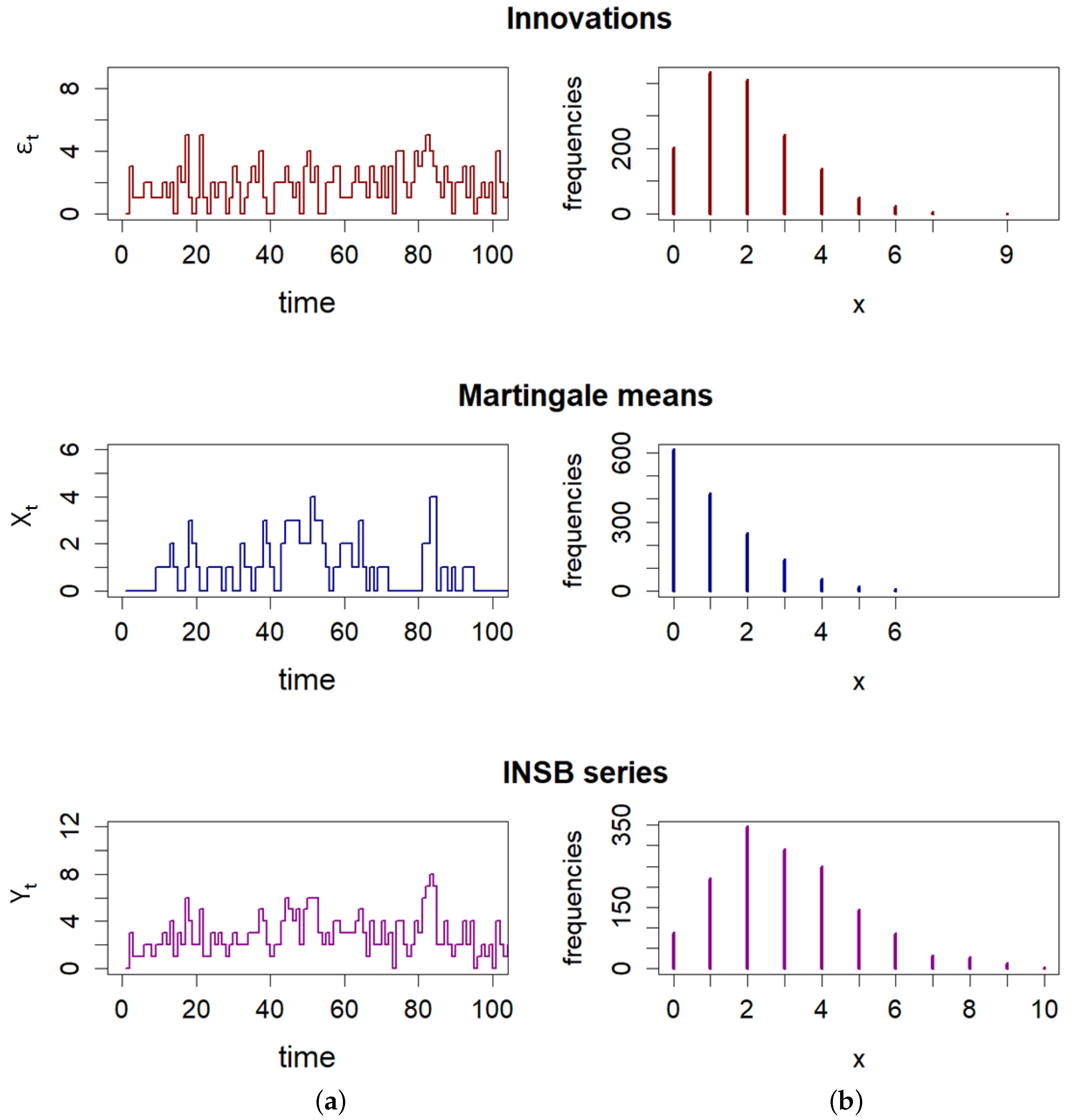
Figure 1 shows realizations of all mentioned INSB series, where as PS-distributed innovations, the Poisson distribution with parameter $a=2$ is taken. It is easy to see that the series $\left(X_t\right)$ of martingale means has the most pronounced zero inflation, which will be formally confirmed further on.

3. Main Properties of the INSB(1) Process

Here, some stochastic features of the INSB(1) process are examined. The following statement gives the integer-valued moving average representation of the infinite order (abbr. INMA$(\infty )$ representation) of corresponding series of this process.

Theorem 1.

Suppose that PS-innovations $\left({\epsilon }_t\right)$, given by Equation (1), have finite first moment ${\mu }_{\epsilon }={\mu }_{\epsilon }\left(a\right)$, which is uniformly bounded on $a\in (0,R)$. Then, the INSB(1) series $\left(X_t\right)$, defined by Equation (3), has an INMA$(\infty )$ representation:

$$X_t\stackrel{d}{=}\sum _{k=1}^{\infty }{\alpha }^k\circ {\xi }_{t-k},$$

(6)

where ${\xi }_t=q_t{\epsilon }_t$, $t\in \mathbb{Z}$. Similarly, series $\left(Y_t\right)$, defined by Equation (5), has a representation:

$$Y_t\stackrel{d}{=}{\epsilon }_t+\sum _{k=1}^{\infty }{\alpha }^k\circ {\xi }_{t-k},$$

(7)

where both sums above converge almost surely.

Proof. 

Using a similar procedure to that in Stojanović et al. [19] (see Theorem 2.1), it can be proved that RVs $\left({\xi }_t\right)$ are mutually uncorrelated with the mean and variance, respectively,

$$\begin{array}{cc}\hfill {\mu }_{\xi }& :=\mathrm{E}\left[{\xi }_t\right]=\mathrm{E}\left[q_t\right]\mathrm{E}\left[{\epsilon }_t\right]={\mu }_q{\mu }_{\epsilon }\left(a\right)={\mu }_{q}ag{}^{\prime }\left(a\right)\hfill \\ \hfill {\sigma }_{\xi }^2& :=\mathrm{Var}\left[{\xi }_t\right]=\mathrm{E}\left[{\xi }_t^2\right]-{\mu }_{\xi }^2={\mu }_q\frac{a{f}^{\prime }\left(a\right)+a^2{f}^{″}\left(a\right)}{f\left(a\right)}-{\mu }_q^2{\left(a\frac{f^{\prime }\left(a\right)}{f\left(a\right)}\right)}^2\hfill \\ & ={\mu }_{q}a\frac{f^{\prime }\left(a\right)}{f\left(a\right)}+{\mu }_q{a}^2\frac{f^{″}\left(a\right)f\left(a\right)-{\mu }_q{\left(f^{\prime }\left(a\right)\right)}^2}{{\left(f\left(a\right)\right)}^2}\hfill \\ & ={\mu }_{\xi }+{\mu }_q{a}^2\left[g^{″}\left(a\right)+F_{\epsilon }\left(c\right){\left(g^{\prime }\left(a\right)\right)}^2\right],\hfill \end{array}$$

(8)

where ${\mu }_q:=\mathrm{E}\left[q_t\right]=P\{{\epsilon }_t\ge c\}=1-F_{\epsilon }\left(c\right)$ and $F_{\epsilon }\left(c\right):=P\{{\epsilon }_t<c\}$ is the cumulative distribution function (CDF) of RVs $\left({\epsilon }_t\right)$. Further, according to assumptions of the theorem, there is an $L>0$ such that

$$\sum _{k=1}^{\infty }P\{{\epsilon }_t\ge k\}=\sum _{k=1}^{\infty }kP\left\{{\epsilon }_t=k\right\}={\mu }_{\epsilon }\left(a\right)\le L<+\infty ,\forall a\in (0,R).$$

Based on that and independence of RVs ${\epsilon }_t$ and $q_t$, for each $t\in \mathbb{Z}$, it follows that

$$\begin{array}{cc}\hfill \sum _{k=1}^{\infty }P\{{\xi }_t\ge k\}& =\sum _{k=1}^{\infty }P\{{\epsilon }_t\ge k\}P\{q_t=1\}=P\{{\epsilon }_t\ge c\}\sum _{k=1}^{\infty }kP\{{\epsilon }_t=k\}\hfill \\ \hfill & ={\mu }_q{\mu }_{\epsilon }\left(a\right)\le {\mu }_{q}L<+\infty ,\hfill \end{array}$$

where the sum above converges uniformly on $a\in (0,R)$. In addition, as $1/k$, $k=1,2,\dots$ is a monotone and bounded sequence, the Abelian criterion for convergence of infinite sums implies that

$$\sum _{k=1}^{\infty }\frac{1}{k}P\{{\xi }_t\ge k\}={\mu }_q\sum _{k=1}^{\infty }\frac{1}{k}P\{{\epsilon }_t\ge k\}<+\infty .$$

(9)

Moreover, the above convergence is uniform on $a\in (0,R)$, and using Theorem 2.1 in Alzaid and Al-Osh [22], it follows that inequality (9) is sufficient for the equality

$$G_X(u;\theta )=\prod _{k=1}^{\infty }{G}_{\xi }\left(1+{\alpha }^k(u-1);{\theta }_{\xi }\right),$$

(10)

where

$$G_{\xi }(u;{\theta }_{\xi }):=\mathrm{E}\left[u^{{\xi }_t}\right]=1+{\mu }_q\left(\frac{f\left(au\right)}{f\left(a\right)}-1\right)$$

(11)

is the PGF of RVs $\left({\xi }_t\right)$, $G_X(u;\theta ):=\mathrm{E}\left[u^{X_t}\right]$ is the PGF of RVs $\left(X_t\right)$, while ${\theta }_{\xi }={(a,{\mu }_q)}^{\prime }$ and $\theta :={(a,\alpha ,{\mu }_q)}^{\prime }$ are vectors of (unknown) parameters. Furthermore, the above product absolutely converges for every $u\in [-1,1]$, so using the bijective correspondence between PGFs and PMFs of arbitrary RVs, it follows that Equation (10) is equivalent to the INMA$(\infty )$ representation in Equation (6).

To prove the almost sure convergence in Equation (6), note that using Equation (3), for any $k=1,2,\dots$, it holds that

$$X_t\stackrel{d}{=}{\alpha }^k\circ X_{t-k}+\sum _{j=1}^k{\alpha }^j\circ {\xi }_{t-j}.$$

(12)

Now, let us consider a random event:

$$\begin{array}{cc}\hfill A& :=\left\{\underset{k\to \infty }{lim}\sum _{j=1}^k{\alpha }^j\circ {\xi }_{t-j}=X_t\right\}=\left\{\underset{k\to \infty }{lim}{\alpha }^k\circ X_{t-k}=0\right\}=\bigcap _{\delta >0}\bigcup _{n=1}^{\infty }\bigcap _{k=n}^{\infty }\left\{0\le {\alpha }^k\circ X_{t-k}<\delta \right\}\hfill \\ & =\bigcup _{n=1}^{\infty }\bigcap _{k=n}^{\infty }\left\{{\alpha }^k\circ X_{t-k}=0\right\}=\bigcup _{n=1}^{\infty }{A}_n,\hfill \end{array}$$

where $A_n:={\bigcap }_{k=n}^{\infty }\{{\alpha }^k\circ X_{t-k}=0\}.$ According to Equation (12), for any $m,n=1,2,\dots$, one obtains

$${\alpha }^n\circ X_{t-n}\stackrel{d}{=}{\alpha }^{m+n}\circ X_{t-m-n}+\sum _{j=n+1}^{m+n}{\alpha }^j\circ {\xi }_{t-j}.$$

From here, using the probability continuity property and the definition of the thinning operator, for events $A_n$, we obtain

$$\begin{array}{cc}\hfill P\left(A_n\right)& =P\left(\underset{m\to \infty }{lim}\bigcap _{k=n}^{m+n}\left\{{\alpha }^k\circ X_{t-k}=0\right\}\right)\hfill \\ & =\underset{m\to \infty }{lim}\left(P\left\{{\alpha }^{m+n}\circ X_{t-m-n}=0\right\}\times \prod _{j=n+1}^{m+n}P\left\{{\alpha }^j\circ {\xi }_{t-j}=0\right\}\right)\hfill \\ & =\underset{m\to \infty }{lim}\left(\sum _{k=0}^{\infty }{\left(1-{\alpha }^{m+n}\right)}^{k}P\left\{X_{t-m-n}=k\right\}\right)\times \underset{m\to \infty }{lim}\prod _{j=n+1}^{m+n}\left(\sum _{k=0}^{\infty }{\left(1-{\alpha }^j\right)}^{k}P\left\{{\xi }_{t-j}=k\right\}\right)\hfill \\ & =\underset{m\to \infty }{lim}{G}_X(1-{\alpha }^{m+n};\theta )\times \underset{m\to \infty }{lim}\prod _{j=n+1}^{m+n}{G}_{\xi }(1-{\alpha }^j;{\theta }_{\xi })\hfill \\ & =G_X(1;\theta )\times \prod _{j=n+1}^{\infty }{G}_{\xi }(1-{\alpha }^j;{\theta }_{\xi })\hfill \\ & =\prod _{j=n+1}^{\infty }{G}_{\xi }(1-{\alpha }^j;{\theta }_{\xi }).\hfill \end{array}$$

By applying again the property of continuity of probability and convergence of the product in Equation (10), it follows that

$$P\left(A\right)=\underset{n\to \infty }{lim}P\left(A_n\right)=\underset{n\to \infty }{lim}\prod _{j=n+1}^{\infty }{G}_{\xi }(1-{\alpha }^j;{\theta }_{\xi })=1,$$

that is, the sum in Equation (6) converges almost surely. Similarly, using the definition of the series $\left(Y_t\right)$, given by Equation (5), the almost sure convergence in Equation (7) is proved. □

Remark 1

(PGFs of the INSB series). By applying a procedure similar to the previous theorem, as well as some general facts about PGFs of non-negative stationary integer-valued time series (see, e.g., [20]), explicit expressions for the PGFs of the INSB(1) process can be obtained. Namely, using Equations (5), (10) and (11), the first-order PGFs of the series $\left(X_t\right)$ and $\left(Y_t\right)$ are

$$\begin{array}{cc}\hfill G_X(u;\theta )& =\prod _{k=1}^{\infty }\left[1+{\mu }_q\left(\frac{f\left((1+{\alpha }^k(u-1))a\right)}{f\left(a\right)}-1\right)\right],\hfill \\ \hfill G_Y(u;\theta )& =G_{\epsilon }(u;\theta )G_X(u;\theta )=\frac{f\left(au\right)}{f\left(a\right)}\prod _{k=1}^{\infty }\left[1+{\mu }_q\left(\frac{f\left((1+{\alpha }^k(u-1))a\right)}{f\left(a\right)}-1\right)\right].\hfill \end{array}$$

(13)

Furthermore, suppose that $\mathbf{u}={(u_1,\dots ,u_r)}^{\prime }\in {\mathbf{R}}^r$, $r\ge 2$, and ${\mathbf{X}}_t^{\left(r\right)}:={(X_t,\dots ,X_{t+r-1})}^{\prime }$, ${\mathbf{Y}}_t^{\left(r\right)}:={(Y_t,\dots ,Y_{t+r-1})}^{\prime }$, $t\in \mathbb{Z}$, are the overlapping blocks of series $\left(X_t\right)$ and $\left(Y_t\right)$, respectively. The replacement $k=1,\dots ,r-1$ in Equation (12) and some calculations give the r-dimensional PGFs of random vectors ${\mathbf{X}}_t^{\left(r\right)}$ and ${\mathbf{Y}}^{\left(r\right)}$ as follows:

$$\begin{array}{cc}\hfill G_X^{\left(r\right)}(\mathbf{u};\theta )& :=\mathrm{E}\left[u_1^{X_t}\cdots u_r^{X_{t+r-1}}\right]\hfill \\ & =G_X\left(\prod _{k=0}^{r-1}\left(1+{\alpha }^k(u_{k+1}-1)\right);\theta \right)\hfill \\ & \times \prod _{\ell =2}^r\left[1+{\mu }_q\left(\frac{f\left({\prod }_{k=0}^{r-\ell }\left(1+{\alpha }^{k+1}(u_{k+\ell }-1)\right)a\right)}{f\left(a\right)}-1\right)\right]\hfill \\ \mathrm{and}\hfill G_Y^{\left(r\right)}(\mathbf{u};\theta )& :=\mathrm{E}\left[u_1^{Y_t}\cdots u_r^{Y_{t+r-1}}\right]\hfill \\ \hfill & =G_X\left(\prod _{k=0}^{r-1}\left(1+{\alpha }^k(u_{k+1}-1)\right);\theta \right)\hfill \\ \hfill & \times \prod _{\ell =1}^r\left[\frac{(1-{\mu }_q)f\left(a{u}_{\ell }\right)+{\mu }_{q}f\left({\prod }_{k=0}^{r-\ell }\left(1+{\alpha }^k(u_{k+\ell }-1)\right)a\right)}{f\left(a\right)}\right].\hfill \end{array}$$

(14)

Also, it is worth noting that by using realizations of the (only) observable series $\left(Y_t\right)$, that is, the second-order PGF $G_Y^{\left(2\right)}(\mathbf{u};\theta )$, the parameter estimators of the INSB(1) process will be obtained (see Section 4, below).

Based on the previous theorem, the following statement concerns the mean, variance and correlation structure of INSB series.

Theorem 2.

Assume that the conditions of Theorem 1 hold, as well as that series $\left(X_t\right)$ and $\left(Y_t\right)$, given by Equations (3) and (5), respectively, have second-order finite moments. Then, both of these series are strictly stationary and ergodic. The mean and variance for the series $\left(X_t\right)$ are, respectively,

$$\begin{array}{cc}\hfill {\mu }_X& :=\frac{\alpha {\mu }_q}{1-\alpha }a{g}^{\prime }\left(a\right),\hfill \\ \hfill {\sigma }_X^2& :={\mu }_X+\frac{{\alpha }^2{a}^2{\mu }_q}{1-{\alpha }^2}\left[g^{″}\left(a\right)+F_{\epsilon }\left(c\right){\left(g^{\prime }\left(a\right)\right)}^2\right],\hfill \end{array}$$

(15)

and the autocorrelation function (ACF) is ${\rho }_X\left(k\right)={\alpha }^k$, $k=0,1,\dots$ Similarly, for the series $\left(Y_t\right)$, it is

$$\begin{array}{cc}\hfill {\mu }_Y& :=\frac{(1-\alpha F_{\epsilon }\left(c\right))}{1-\alpha }a{g}^{\prime }\left(a\right),\hfill \\ \hfill {\sigma }_Y^2& :={\mu }_Y+\frac{a^2}{1-{\alpha }^2}\left[g^{″}\left(a\right)\left(1-{\alpha }^2{F}_{\epsilon }\left(c\right)\right)+{\alpha }^2{F}_{\epsilon }\left(c\right)(1-F_{\epsilon }\left(c\right)){\left(g^{\prime }\left(a\right)\right)}^2\right],\hfill \end{array}$$

(16)

and its ACF is

$${\rho }_Y\left(k\right)=\left\{\begin{array}{cc}1,\hfill & k=0,\hfill \\ {\displaystyle \frac{{\alpha }^k\left({\sigma }_X^2+{\mu }_q{\sigma }_{\epsilon }^2\right)}{{\sigma }_X^2+{\sigma }_{\epsilon }^2},}\hfill & k=1,2,\dots \hfill \end{array}\right.$$

Additionally, both sums in their INMA(∞) representations, given by Equations (6) and (7), converge in the mean-square sense.

Proof. 

Using Equation (6) and the well-known features of the binomial thinning operator (see, e.g., Kella & Löpker [23]), for the mean of the series $\left(X_t\right)$, one obtains

$${\mu }_X=\mathrm{E}\left[X_t\right]=\sum _{j=1}^{\infty }\mathrm{E}\left[{\alpha }^j\circ {\xi }_{t-j}\right]={\mu }_{\xi }\sum _{j=1}^{\infty }{\alpha }^j=\frac{\alpha {\mu }_{\xi }}{1-\alpha }.$$

Analogously, the variance of this series is obtained as follows:

$$\begin{array}{cc}\hfill {\sigma }_X^2& =\mathrm{Var}\left[X_t\right]=\sum _{j=1}^{\infty }\mathrm{Var}\left[{\alpha }^j\circ {\xi }_{t-j}\right]=\sum _{j=1}^{\infty }\left({\alpha }^{2j}\mathrm{Var}\left[{\xi }_{t-j}\right]+{\alpha }^j\left(1-{\alpha }^j\right)\mathrm{E}\left[{\xi }_{t-j}\right]\right)\hfill \\ & =\frac{{\alpha }^2{\sigma }_{\xi }^2}{1-{\alpha }^2}+\left(\frac{\alpha }{1-\alpha }-\frac{{\alpha }^2}{1-{\alpha }^2}\right){\mu }_{\xi }=\frac{\alpha {\mu }_{\xi }}{1-{\alpha }^2}+\frac{{\alpha }^2{\sigma }_{\xi }^2}{1-{\alpha }^2}.\hfill \end{array}$$

From here, by substituting Equations (8) for the mean value (${\mu }_{\xi }$) and variance (${\sigma }_{\xi }^2$) of the series $\left({\xi }_t\right)$, and after some computations, Equations (15) are obtained. Finally, according to Equation (12), the ACF of the series $\left(X_t\right)$ is obtained from the equalities

$$\begin{array}{cc}\hfill {\rho }_X\left(k\right)& :=\mathrm{Corr}\left[X_t,X_{t+k}\right]=\mathrm{Corr}\left[X_t,{\alpha }^k\circ X_t\right]+\sum _{j=1}^k\mathrm{Corr}\left[X_t,{\alpha }^j\circ {\xi }_{t+k-j}\right]={\alpha }^k,k=0,1,\dots \hfill \end{array}$$

Note that previously proven facts imply that RVs $\left(X_t\right)$ have finite moments up to the second order. Then, using again Equation (12) and features of the binomial thinning, one obtains

$$\mathrm{E}{\left[X_t-\sum _{j=1}^k{\alpha }^j\circ {\xi }_{t-j}\right]}^2=\mathrm{E}{\left[{\alpha }^k\circ X_{t-k}\right]}^2={\alpha }^{2k}\mathrm{E}\left[X_{t-k}^2\right]+{\alpha }^k(1-{\alpha }^k)\mathrm{E}\left[X_{t-k}\right]⟶0,k\to \infty .$$

Thus, the mean-square convergence of the sum in Equation (6) holds. Finally, the statement for the series $\left(Y_t\right)$ can be proved in a completely analogous way. □

According to the previous theorem, in the non-trivial case $0<{\mu }_q<1$, the inequalities ${\rho }_Y\left(k\right)<{\rho }_X\left(k\right)$, $k=1,2,\dots$ obviously hold. Therefore, the basic INSB series $\left(Y_t\right)$ has a weaker correlation than $\left(X_t\right)$, i.e., compared with the correlation of INAR-based models. Also, by applying the previous results, the over-dispersion conditions for INSB series can be described as follows.

Remark 2

(Over-dispersion conditions). Recall that the over-dispersion of the PS series $\left({\epsilon }_t\right)$ depends on the function $g\left(a\right)=lnf\left(a\right)$. Namely, Equations (2) imply that $D_{\epsilon }\left(a\right):={\sigma }_{\epsilon }^2-{\mu }_{\epsilon }>0$ if and only if $g^{″}\left(a\right)>0$, $\forall a\in (0,R).$ On the other hand, the over-dispersion conditions of the series $\left({\xi }_t\right)$ are weaker, because Equations (8) imply that $D_{\xi }\left(a\right):={\sigma }_{\xi }^2-{\mu }_{\xi }>0$ holds if and only if

$$g^{″}\left(a\right)\ge 0or{F}_{\epsilon }\left(c\right)>-\frac{g^{″}\left(a\right)}{{\left(g^{\prime }\left(a\right)\right)}^2}.$$

Thereafter, using Theorem 2, that is, Equations (15), it is obtained that

$$D_X\left(a\right):={\sigma }_X^2-{\mu }_X=\frac{{\alpha }^2{D}_{\xi }\left(a\right)}{1-{\alpha }^2},$$

so the over-dispersion conditions are the same for both series $\left(X_t\right)$ and $\left({\xi }_t\right)$. Finally, Equation (16) implies that $D_Y\left(a\right):={\sigma }_Y^2-{\mu }_Y>0$ if and only if

$$g^{″}\left(a\right)\ge 0or\frac{{\alpha }^2{F}_{\epsilon }\left(c\right)\left(1-F_{\epsilon }\left(c\right)\right)}{1-{\alpha }^2{F}_{\epsilon }\left(c\right)}>-\frac{g^{″}\left(a\right)}{{\left(g^{\prime }\left(a\right)\right)}^2}.$$

According to the inequality ${\alpha }^{2}x(1-x)/(1-{\alpha }^{2}x)<x$, $\forall \alpha ,x\in (0,1)$, it follows that

$$F_{\epsilon }\left(c\right)>\frac{{\alpha }^2{F}_{\epsilon }\left(c\right)\left(1-F_{\epsilon }\left(c\right)\right)}{1-{\alpha }^2{F}_{\epsilon }\left(c\right)}.$$

Thus, over-dispersion of the series $\left(Y_t\right)$ implies over-dispersion for $\left(X_t\right)$, that is, $\left(X_t\right)$ has weaker over-dispersion conditions than $\left(Y_t\right)$.

The Markov properties of the INSB(1) series, their marginal distributions and the properties of zero inflation are discussed below.

Theorem 3.

Let $\left({\epsilon }_t\right)$ be the PS-distributed series, with the PMF given by Equation (1). The martingale mean series $\left(X_t\right)$, defined by Equation (3), is a homogeneous Markov process with one-step transition probabilities:

$$\begin{array}{cc}\hfill p_{i,j}^{\left(X\right)}:=P\left\{X_t=j|X_{t-1}=i\right\}& =F_{\epsilon }\left(c\right)\left(\genfrac{}{}{0pt}{}{i}{j}\right){\alpha }^j{(1-\alpha )}^{i-j}I\left(i\ge j\right)+(1-F_{\epsilon }\left(c\right))\hfill \\ \hfill & \times \sum _{k=0}^{\infty }\left(\genfrac{}{}{0pt}{}{i+k}{j}\right){\alpha }^j{(1-\alpha )}^{i+k-j}{p}_{\epsilon }(k;a)I\left(i+k\ge j\right).\hfill \end{array}$$

(17)

Similarly, series $\left(Y_t\right)$, given by Equation (5), is a Markov process with transition probabilities:

$$\begin{array}{cc}\hfill p_{i,j}^{\left(Y\right)}& :=P\left\{Y_t=j|Y_{t-1}=i\right\}=\sum _{k=0}^m\left(\genfrac{}{}{0pt}{}{i}{k}\right){\alpha }^k{(1-\alpha )}^{i-k}{p}_{\eta }(j-k;\theta ),\hfill \end{array}$$

(18)

where $m=min\{i,j\}$ and

$$p_{\eta }(x;\theta ):=\left(1-F_{\epsilon }\left(c\right)\right)p_{\epsilon }(x;a)+F_{\epsilon }\left(c\right)\sum _{k=0}^{\infty }\sum _{\ell =k}^{\infty }\left(\genfrac{}{}{0pt}{}{\ell }{k}\right){\alpha }^k{(1-\alpha )}^{\ell -k}{p}_{\epsilon }(x+k;a)p_{\epsilon }(\ell ;a)$$

(19)

is the PMF of the series ${\eta }_t:={\epsilon }_t-\alpha \circ {\epsilon }_{t-1}(1-q_{t-1})$, $t\in \mathbb{Z}$.

Proof. 

Using Equations (3) and (4), as well as the definition of conditional probabilities and binomial thinning, for the conditional distribution of $X_t$ on a given $X_{t-1}$, one obtains

$$\begin{array}{cc}\hfill p_{i,j}^{\left(X\right)}& =P\left\{\alpha \circ \left(X_{t-1}+{\xi }_{t-1}\right)=j|X_{t-1}=i\right\}\hfill \\ & =P\left\{\alpha \circ X_{t-1}=j|X_{t-1}=i\right\}P\{q_{t-1}=0\}\hfill \\ & +P\left\{\alpha \circ \left(X_{t-1}+{\epsilon }_{t-1}\right)=j|X_{t-1}=i\right\}P\{q_{t-1}=1\}\hfill \\ & =F\epsilon \left(c\right)p_i(j;\alpha )I\left(i\ge j\right)+\left(1-F\epsilon \left(c\right)\right)\sum _{k=0}^{\infty }P\left\{\alpha \circ \left(X_{t-1}+k\right)=j|X_{t-1}=i\right\}{p}_{\epsilon }(k;a)\hfill \\ & =F\epsilon \left(c\right)p_i(j;\alpha )I\left(i\ge j\right)+(1-F\epsilon \left(c\right))\sum _{k=0}^{\infty }{p}_{i+k}(j;\alpha )p_{\epsilon }(k;a)I\left(i+k\ge j\right),\hfill \end{array}$$

where

$$p_i(j;\alpha ):=\left(\genfrac{}{}{0pt}{}{i}{j}\right){\alpha }^j{(1-\alpha )}^{i-j},j=0,1,\dots ,i$$

is the PMF of binomial distribution $\mathcal{B}(i;\alpha )$. From here, Equation (17) is directly obtained.

On the other hand, notice that for the series $\left(Y_t\right)$, it is valid that

$$\begin{array}{cc}\hfill Y_t=X_t+{\epsilon }_t& =\alpha \circ \left(X_{t-1}+q_{t-1}{\epsilon }_{t-1}\right)+{\epsilon }_t=\alpha \circ \left(Y_{t-1}-{\epsilon }_{t-1}+q_{t-1}{\epsilon }_{t-1}\right)+{\epsilon }_t\hfill \\ \hfill & \stackrel{d}{=}\alpha \circ Y_{t-1}+{\eta }_t,\hfill \end{array}$$

(20)

where using conditional probabilities, the PMF of the series $\left({\eta }_t\right)$ is obtained as follows:

$$\begin{array}{cc}\hfill p_{\eta }(x;\theta )& =P\left\{{\epsilon }_t=x\right\}P\{q_{t-1}=1\}+P\left\{{\epsilon }_t-\alpha \circ {\epsilon }_{t-1}=x\right\}P\{q_{t-1}=0\}\hfill \\ \hfill & =\left(1-F_{\epsilon }\left(c\right)\right)p_{\epsilon }(x;a)+F_{\epsilon }\left(c\right)\sum _{k=0}^{\infty }P\left\{{\epsilon }_t=x+k\right\}P\left\{\alpha \circ {\epsilon }_{t-1}=k\right\}\hfill \\ \hfill & =\left(1-F_{\epsilon }\left(c\right)\right)p_{\epsilon }(x;a)+F_{\epsilon }\left(c\right)\sum _{k=0}^{\infty }{p}_{\epsilon }(x+k;a)\sum _{\ell =0}^{\infty }{p}_{\ell }(k;\alpha )p_{\epsilon }(\ell ;a)I\left(\ell \ge k\right).\hfill \end{array}$$

It can easily be seen that the last obtained equality is equivalent to Equation (19). According to this, for the conditional distribution of $Y_t$ on a given $Y_{t-1}$, one obtains

$$\begin{array}{cc}\hfill p_{i,j}^{\left(Y\right)}& =P\left\{\alpha \circ Y_{t-1}+{\eta }_t=j|Y_{t-1}=i\right\}=\sum _{k=0}^{m}P\left\{\alpha \circ Y_{t-1}=k|Y_{t-1}=i\right\}{p}_{\eta }(j-k;\theta )\hfill \\ & =\sum _{k=0}^m{p}_i(k;\alpha )p_{\eta }(j-k;\theta ),\hfill \end{array}$$

which proves Equation (18), as well as the theorem completely. □

Remark 3

(Distributional properties). Note that the first summand in Equation (17) exists if and only if martingale means $\left(X_t\right)$ pass from the state $X_{t-1}=i$ to the non-increasing state $X_t=j\le i$. In addition, the transition probabilities given by Equations (17) and (18) give the marginal PMFs of the INSB series $\left(X_t\right)$ and $\left(Y_t\right)$:

$$\begin{array}{cc}\hfill p_X(x;\theta ):=P\left\{X_t=x\right\}& =\sum _{k=0}^{\infty }P\left\{X_t=x|X_{t-1}=k\right\}P\left\{X_{t-1}=k\right\}=\sum _{k=0}^{\infty }{p}_{k,x}^{\left(X\right)}{p}_X(k;\theta ),\hfill \\ \hfill p_Y(y;\theta ):=P\left\{Y_t=y\right\}& =\sum _{k=0}^{\infty }P\left\{Y_t=y|Y_{t-1}=k\right\}P\left\{Y_{t-1}=k\right\}=\sum _{k=0}^{\infty }{p}_{k,y}^{\left(Y\right)}{p}_Y(k;\theta ).\hfill \end{array}$$

Finally, using the PGFs of the INSB series $\left(X_t\right)$ and $\left(Y_t\right)$, given by Equations (13), the PMFs of these two series can also be expressed as follows:

$$\begin{array}{cc}\hfill p_X(k;\theta )& =\frac{1}{k!}\frac{{\partial }^k{G}_Y(u;\theta )}{\partial u^k}{|}_{u=0},p_Y(k;\theta )=\frac{1}{k!}\frac{{\partial }^k{G}_Y(u;\theta )}{\partial u^k}{|}_{u=0}.\hfill \end{array}$$

(21)

In a similar way to INAR processes with zero inflation (see, e.g., Li et al. [24,25]), the distribution of zero lengths of INSB(1) processes is examined below. For this purpose, recall that we have assumed that the condition $0\in \mathit{S}$ is satisfied and observe the distribution of zero “runs”, as the number of zeros occurrences between two distinct non-zero values. The following statement gives the expected lengths of zeros in INSB(1) model.

Theorem 4.

The expected lengths of zero runs for the series $\left(X_t\right)$ and $\left(Y_t\right)$ are, respectively,

$$\begin{array}{cc}\hfill {\mathcal{L}}_0^{\left(X\right)}& =\frac{f\left(a\right)-{\mu }_q\left[f\left(a\right)-f\left(a\right(1-\alpha \left)\right)\right]}{{\mu }_q\left[f\left(a\right)-f\left(a\right(1-\alpha \left)\right)\right]},\hfill \\ \hfill {\mathcal{L}}_0^{\left(Y\right)}& =\frac{p_{\eta }\left(0\right)}{1-p_{\eta }\left(0\right)},\hfill \end{array}$$

(22)

where ${\mu }_q:=1-F_{\epsilon }\left(c\right)$ and $p_{\eta }\left(0\right)$ is the proportion of zeros in the RVs $\left({\eta }_t\right)$.

Proof. 

Using Equation (17), as well as Equation (1) for the PS distributions family, the probabilities of transitions from zero to zero and from zero to non-zero values of the series $\left(X_t\right)$ are obtained as follows:

$$\begin{array}{cc}\hfill p_0^{\left(X\right)}& :=P\left\{X_t=0|X_{t-1}=0\right\}=F_{\epsilon }\left(c\right)+(1-F_{\epsilon }\left(c\right))\sum _{k=0}^{\infty }{(1-\alpha )}^k{p}_{\epsilon }(k;a)\hfill \\ & =1+{\mu }_q\left[\frac{1}{f\left(a\right)}\sum _{k=0}^{\infty }m\left(k\right){\left(a(1-\alpha )\right)}^k-1\right]\hfill \\ & =1+{\mu }_q\left[\frac{f\left(a\right(1-\alpha \left)\right)}{f\left(a\right)}-1\right],\hfill \\ \hfill 1-p_0^{\left(X\right)}& ={\mu }_q\left[1-\frac{f\left(a\right(1-\alpha \left)\right)}{f\left(a\right)}\right].\hfill \end{array}$$

It can easily be seen (see, e.g., Stojanović et al. [21]) that zero lengths of the series $\left(X_t\right)$ have a geometric distribution with parameter $1-p_0^{\left(X\right)}$. Therefore, the expected length of zero is

$${\mathcal{L}}_0^{\left(X\right)}=\frac{p_0^{\left(X\right)}}{1-p_0^{\left(X\right)}},$$

and from here the first equality in Equations (22) immediately follows. Similarly, according to Equation (18) and using the same procedure as the previous one, the second equality in (22) is easily obtained. □

Remark 4

(Zero-inflation properties). Based on the previous results, the proportions of zeros in the INSB series can be easily computed. Indeed, using the definition of series $\left({\epsilon }_t\right)$ and $\left({\xi }_t\right)$, given by Definition 1 and Theorem 1, one obtains

$$\begin{array}{cc}\hfill p_{\epsilon }(0;a)& :=P\left\{{\epsilon }_t=0\right\}=\frac{f\left(0\right)}{f\left(a\right)},\hfill \\ \hfill p_{\xi }(0;{\theta }_{\xi })& :=P\left\{q_t{\epsilon }_t=0\right\}=P\left\{q_t=0\right\}+P\left\{q_t=1\right\}P\left\{{\epsilon }_t=0\right\}=1+{\mu }_q\left[p_{\epsilon }(0;a)-1\right].\hfill \end{array}$$

From here, we obtain

$$p_{\xi }(0;{\theta }_{\xi })-p_{\epsilon }(0;a)=(1-{\mu }_q)\left[1-p_{\epsilon }(0;a)\right]>0,$$

i.e., RVs $\left({\xi }_t\right)$ have a more pronounced zero inflation than $\left({\epsilon }_t\right)$. On the other hand, using the PGFs of the series $\left(X_t\right)$ and $\left(Y_t\right)$, that is, Equations (13) and (21), the zero proportions of these two series are

$$\begin{array}{cc}\hfill p_X(0;\theta )& :=P\left\{X_t=0\right\}=G_X(0;\theta )=\prod _{k=1}^{\infty }\left[1+{\mu }_q\left(\frac{f\left(a(1-{\alpha }^k)\right)}{f\left(a\right)}-1\right)\right],\hfill \\ \hfill p_Y(0;\theta )& :=P\left\{Y_t=0\right\}=G_Y(0;\theta )=\frac{f\left(0\right)}{f\left(a\right)}\prod _{k=1}^{\infty }\left[1+{\mu }_q\left(\frac{f\left(a(1-{\alpha }^k)\right)}{f\left(a\right)}-1\right)\right].\hfill \end{array}$$

Note that these proportions are products of convex combinations of values $f\left(a(1-{\alpha }^k)\right)/f\left(a\right)$, $k=0,1,2,\dots$, and constant 1. Since the function $f\left(a\right)$ is monotonically increasing, it follows that

$$\frac{f\left(0\right)}{f\left(a\right)}<\frac{f\left(a(1-{\alpha }^k)\right)}{f\left(a\right)}<1+{\mu }_q\left(\frac{f\left(a(1-{\alpha }^k)\right)}{f\left(a\right)}-1\right)<1,k=1,2,\dots$$

and this implies $p_Y(0;\theta )<p_{\epsilon }(0;\theta )<p_X(0;\theta ).$ Thus, the basic INSB series $\left(Y_t\right)$ has a less pronounced zero inflation compared with the other mentioned series. Finally, martingale means $\left(X_t\right)$ have the most pronounced zero inflation and can be an adequate stochastic model in the fitting real-world series with pronounced zero values.

4. Parameter Estimation Procedure

Due to the specific structure of the INSB(1) process, its parameter estimation procedure is more complex compared with most known count time-series models. For instance, according to Equation (20), it follows that the (only) observable series $\left(Y_t\right)$ has an INAR(1) structure, but with 1-dependent innovations ${\eta }_t:={\epsilon }_t-\alpha \circ {\epsilon }_{t-1}(1-q_{t-1})$. Therefore, the conditional mean of this series is

$$\mathrm{E}\left[Y_{t+1}|Y_t\right]=\alpha Y_t+{\mu }_{\epsilon }-\alpha \circ {\epsilon }_t(1-q_t),$$

and it depends on realizations of (unobservable) noise indicator $q_t=q_t\left(c\right)$. Thus, some of the widely used estimation methods, e.g., conditional last squares (CLS) method [26], as well as conditional maximum likelihood (CML) method [27], cannot be used here. Moreover, according to Theorem 2 and Equations (15) and (16), it is clear that even some moment-based estimation methods, i.e., the well-known Yule–Walker (YW) estimators [28], cannot simply obtain the above (see Section 6).

In order to obtain efficient parameter estimators of the INSB(1) process, an estimation technique called probability-generating function (PGF) method is examined here. It is worth to notice that some general results of PGF estimation theory were given in Esquivel [29]. Thereafter, some more specific PGF estimation procedures were recently examined in Stojanović et al. [19,20,21], as well as in Cadena et al. [30]. Also, it can be emphasized that the main idea of the PGF method is close to the empirical characteristic function (ECF) estimation method introduced by Yu [31]. Similar to the ECF method, the goal of the PGF method is minimizing the “distance” between the theoretical PGF of the series $\left(Y_t\right)$, given by Equation (14), and its appropriate empirical PGF (of order $r\in \mathbf{N})$:

$${\tilde{G}}_T^{\left(r\right)}\left(\mathbf{u}\right):=\frac{1}{T-r+1}\sum _{t=1}^{T-r+1}{u}_1^{Y_t}\cdots u_r^{Y_{t+r-1}}.$$

(23)

where $\mathbf{u}={(u_1,\dots ,u_r)}^{\prime }\in {\mathbf{R}}^r$ and $\{Y_1,Y_2,\dots ,Y_T\}$ is a finite realization of the basic INSB(1) series $\left(Y_t\right)$. Since the stationarity and ergodicity of the series $\left(Y_t\right)$ was proved in Theorem 2, it follows that

$$\mathrm{E}\left[{\tilde{G}}_T^{\left(r\right)}\left(\mathbf{u}\right)\right]=G_Y^{\left(r\right)}(\mathbf{u};{\theta }_0),$$

(24)

where ${\theta }_0\in (0,R)\times {(0,1)}^2$ is the true value of unknown parameters $\theta ={(a,\alpha ,{\mu }_q)}^{\prime }$. Hence, ${\tilde{G}}_T^{\left(r\right)}\left(\mathbf{u}\right)$ is an unbiased estimator of $G_Y^{\left(r\right)}(\mathbf{u};{\theta }_0)$. In addition, the PGF $G_Y^{\left(r\right)}(\mathbf{u};\theta )$ is well defined on the set ${[-1,1]}^r$, so the objective function can be given as follows:

$$Q_T^{\left(r\right)}\left(\theta \right):={\int }_{-1}^1\cdots {\int }_{-1}^{1}w\left(\mathbf{u}\right){\left(G_Y^{\left(r\right)}(\mathbf{u};\theta )-{\tilde{G}}_T^{\left(r\right)}\left(\mathbf{u}\right)\right)}^2\mathrm{d}\mathbf{u},$$

(25)

where $\mathrm{d}\mathbf{u}:=\mathrm{d}{u}_1\cdots \mathrm{d}{u}_r$ and $w:{\mathbb{R}}^r\to {\mathbb{R}}^{+}$ is a weight function, integrable on ${[-1,1]}^r$. Then, PGF estimators are usually obtained through minimization of the objective function given by Equation (24), with respect to parameters $\theta$. More precisely, PGF estimates are solutions to the equation

$${\widehat{\theta }}_T=\arg \underset{\theta \in \Theta }{min}{Q}_T^{\left(r\right)}\left(\theta \right),$$

(26)

where $\Theta =(0,R)\times {\left(0,1\right)}^2$ is a parameter space of the regular and stationary INSB(1) process. In order to solve Equation (26), some of the numerical integration procedures can be used, which is described in the next section, Section 5. Similar to Stojanović et al. [20], the following statement examines the strict consistency and asymptotic normality (AN) of PGF estimators of the INSB(1) process under certain regulatory conditions.

Theorem 5.

Let ${\theta }_0$ be the true value of the parameter θ and ${\widehat{\theta }}_T$, $T=1,2,\dots$, be solutions to Equation (26). Additionally, assume that the following regularity conditions hold:

$\left(A_1\right)$

${\theta }_0\in \Theta$ and ${\widehat{\theta }}_T\in \Theta$, for T large enough.

$\left(A_2\right)$

The function

$$Q_0^{\left(r\right)}\left(\theta \right):={\int }_{-1}^1\cdots {\int }_{-1}^{1}w\left(\mathbf{u}\right){\left(G_Y^{\left(r\right)}(\mathbf{u};\theta )-G_Y^{\left(r\right)}(\mathbf{u};{\theta }_0)\right)}^2\mathrm{d}\mathbf{u}$$

has a unique minimum $Q_0^{\left(r\right)}\left({\theta }_0\right)=0$ at the point $\theta ={\theta }_0$.

$\left(A_3\right)$

${\displaystyle \frac{\partial G_Y^{\left(r\right)}(\mathbf{u};{\theta }_0)}{\partial \theta }}{\displaystyle \frac{\partial G_Y^{\left(r\right)}(\mathbf{u};{\theta }_0)}{\partial {\theta }^{\prime }}}$ is a non-zero matrix uniformly bounded by some positive and w-integrable function $\mathcal{W}:{\mathbb{R}}^r\to {\mathbb{R}}^{+}$.

$\left(A_4\right)$

${\displaystyle \frac{{\partial }^2{Q}_T^{\left(r\right)}\left({\theta }_0\right)}{\partial \theta \partial {\theta }^{\prime }}}$ is a regular matrix.

Then, ${\widehat{\theta }}_T$ is a strictly consistent and AN estimator of the parameter θ.

Proof. 

To prove the statement of theorem, we use a procedure based on some general results related to PGF estimators, described in Stojanović et al. [20]. First, the consistency of the estimator ${\widehat{\theta }}_T$ should be checked. As the INSB(1) series $\left(Y_t\right)$ is ergodic, Equation (24) and the strong law of large numbers (SLLN) give

$${\tilde{G}}_T^{\left(r\right)}\left(\mathbf{u}\right)\stackrel{\mathrm{as}}{⟶}{G}_Y^{\left(r\right)}(\mathbf{u};{\theta }_0),T\to \infty .$$

(27)

Furthermore, by assumption $\left(A_1\right)$, the set $\overline{\Theta }=[0,R]\times {[0,1]}^2$ is a compact, with ${\theta }_0$ belonging to its interior. Therefore, the continuous functions $G_Y^{\left(r\right)}(\mathbf{u};\theta )$ and ${\tilde{G}}_T^{\left(r\right)}\left(\mathbf{u}\right)$ are bounded on compacts ${[-1,1]}^r\times \overline{\Theta }$ and ${[-1,1]}^r$, respectively, so that for some $M_1,M_2>0$ is valid:

$$\underset{(\mathbf{u};\theta )\in {[-1,1]}^r\times \overline{\Theta }}{max}|G_Y^{\left(r\right)}(\mathbf{u};\theta )|\le M_1<+\infty ,\underset{\mathbf{u}\in {[-1,1]}^r}{max}\left|{\tilde{G}}_T^{\left(r\right)}\left(\mathbf{u}\right)\right|\le M_2<+\infty .$$

According to this and similarly as in Stojanović et al. [20], it follows that

$$\begin{array}{cc}\hfill |Q_T^{\left(r\right)}\left(\theta \right)-Q_0^{\left(r\right)}\left(\theta \right)|& \le (3M_1+M_2){\int }_{-1}^1\cdots {\int }_{-1}^{1}w\left(\mathbf{u}\right)\left|G_Y^{\left(r\right)}(\mathbf{u};{\theta }_0)-{\tilde{G}}_T^{\left(r\right)}\left(\mathbf{u}\right)\right|\mathrm{d}\mathbf{u},\hfill \end{array}$$

which, along with Equation (27), implies that

$$\underset{\theta \in \overline{\Theta }}{sup}\left|Q_T^{\left(r\right)}\left(\theta \right)-Q_0^{\left(r\right)}\left({\theta }_0\right)\right|\stackrel{\mathrm{as}}{⟶}0,T\to +\infty .$$

Thus, $Q_T^{\left(r\right)}\left(\theta \right)$ converge almost surely and uniformly to $Q_0^{\left(r\right)}\left(\theta \right)$. According to this, as well as assumption $\left(A_2\right)$ and Theorem 2.1 in Newey and McFadden [32], one obtains

$${\widehat{\theta }}_T^{\left(r\right)}-{\theta }_0\stackrel{\mathrm{as}}{⟶}0,T\to +\infty ,$$

that is, ${\widehat{\theta }}_T$ is a strictly consistent estimator of the parameter $\theta$.

In order to prove the property of AN for ${\widehat{\theta }}_T$, note that the partial derivatives up to the first two orders of the function $Q_T^{\left(r\right)}\left(\theta \right)$ are continuous functions. Therefore, they can then be differentiated under the integral sign, as follows:

$$\begin{array}{ccc}\hfill \frac{\partial Q_T^{\left(r\right)}\left(\theta \right)}{\partial \theta }& =& 2{\int }_{-1}^1\cdots {\int }_{-1}^{1}w\left(\mathbf{u}\right)\left[G_Y^{\left(r\right)}(\mathbf{u};\theta )-{\tilde{G}}_T\left(\mathbf{u}\right)\right]\frac{\partial G_Y^{\left(r\right)}(\mathbf{u};\theta )}{\partial \theta }\mathrm{d}\mathbf{u},\hfill \\ \hfill \frac{{\partial }^2{Q}_T^{\left(r\right)}\left(\theta \right)}{\partial \theta \partial {\theta }^{\prime }}& =& 2{\int }_{-1}^1\cdots {\int }_{-1}^{1}w\left(\mathbf{u}\right)\left\{\frac{\partial G_Y^{\left(r\right)}(\mathbf{u};\theta )}{\partial \theta }\frac{\partial G_Y^{\left(r\right)}(\mathbf{u};\theta )}{\partial {\theta }^{\prime }}\right.\hfill \end{array}$$

(28)

$$\begin{array}{ccc}& & \left.+\left[G_Y^{\left(r\right)}(\mathbf{u};\theta )-{\tilde{G}}_T\left(\mathbf{u}\right)\right]\frac{{\partial }^2{G}_Y^{\left(r\right)}(\mathbf{u};\theta )}{\partial \theta \partial {\theta }^{\prime }}\right\}\mathrm{d}\mathbf{u}.\hfill \end{array}$$

(29)

From here, taking the mean values at $\theta ={\theta }_0$, one obtains

$$E\left[\frac{\partial Q_T^{\left(r\right)}\left({\theta }_0\right)}{\partial \theta }\right]={\mathbf{0}}_{r\times 1},E\left[\frac{{\partial }^2{Q}_T^{\left(r\right)}\left({\theta }_0\right)}{\partial \theta \partial {\theta }^{\prime }}\right]=2\mathbf{W},$$

(30)

where

$$\mathbf{W}={\int }_{-1}^1\cdots {\int }_{-1}^{1}w\left(\mathbf{u}\right)\frac{\partial G_Y^{\left(r\right)}(\mathbf{u};{\theta }_0)}{\partial \theta }\frac{\partial G_Y^{\left(r\right)}(\mathbf{u};{\theta }_0)}{\partial {\theta }^{\prime }}\mathrm{d}\mathbf{u}.$$

According to assumption $\left(A_3\right)$, for the function $\mathcal{W}:{\mathbb{R}}^r\to {\mathbb{R}}^{+}$, it is valid that

$$0<∥\frac{\partial G_Y^{\left(r\right)}(\mathbf{u};{\theta }_0)}{\partial \theta }\frac{\partial G_Y^{\left(r\right)}(\mathbf{u};{\theta }_0)}{\partial {\theta }^{\prime }}∥\le \mathcal{W}\left(\mathbf{u}\right),\forall \mathbf{u}\in {[-1,1]}^r,$$

where $∥·∥$ is some matrix norm on ${\mathbb{R}}^r\times {\mathbb{R}}^r$. Therefore, it follows that

$$0<∥\mathbf{W}∥\le {\int }_{-1}^1\cdots {\int }_{-1}^{1}g\left(\mathbf{u}\right)\mathcal{W}\left(\mathbf{u}\right)\mathrm{d}\mathbf{u}<+\infty ,$$

and using Equations (30) and SLLN, it is obtained that

$$\left(\frac{\partial Q_T^{\left(r\right)}\left({\theta }_0\right)}{\partial \theta },\frac{{\partial }^2{Q}_T^{\left(r\right)}\left({\theta }_0\right)}{\partial \theta \partial {\theta }^{\prime }}\right)\stackrel{as}{⟶}(0,2\mathbf{W}),T\to +\infty .$$

(31)

Further, according to Equations (23) and (28), the gradient of function $Q_T^{\left(r\right)}\left(\theta \right)$ is as follows:

$$\frac{\partial Q_T^{\left(r\right)}\left(\theta \right)}{\partial \theta }=\frac{2}{T-r+1}\sum _{t=1}^{T-r+1}{C}_t^{\left(r\right)}\left(\theta \right),$$

(32)

where

$$C_t^{\left(r\right)}\left(\theta \right):={\int }_{-1}^1\cdots {\int }_{-1}^{1}w\left(\mathbf{u}\right)\left[G_Y^{\left(r\right)}(\mathbf{u};\theta )-u_1^{X_t}\cdots u_r^{X_{t+r-1}}\right]\frac{\partial G_Y^{\left(r\right)}(\mathbf{u};\theta )}{\partial \theta }\mathrm{d}\mathbf{u},$$

and $\mathrm{E}\left[C_t^{\left(r\right)}\left({\theta }_0\right)\right]=0$ holds. Using some general facts on ECF theory (see, e.g., [30,31]), absolute summability of covariance ${\gamma }_Y\left(k\right):=\mathrm{Cov}(Y_t,Y_{t+k})$, $k=0,\pm 1,\dots$ of the series $\left(Y_t\right)$ is sufficient for a non-zero finite value:

$$\begin{array}{cc}\hfill {\mathbf{V}}^2& :=\underset{T\to \infty }{lim}\mathrm{Var}\left[\frac{1}{\sqrt{T-r+1}}\sum _{t=1}^{T-r+1}{C}_t^{\left(r\right)}\left({\theta }_0\right)\right]=\underset{T\to \infty }{lim}\frac{1}{T-r+1}\mathrm{E}{\left[\sum _{t=1}^{T-r+1}{C}_t^{\left(r\right)}\left({\theta }_0\right)\right]}^2\hfill \\ & =\underset{T\to \infty }{lim}\frac{1}{{(T-r+1)}^2}\sum _{t=1}^{T-r+1}\sum _{s=1}^{T-r+1}\mathrm{Cov}\left[C_t^{\left(r\right)}\left({\theta }_0\right),C_s^{\left(r\right)}\left({\theta }_0\right)\right].\hfill \end{array}$$

(33)

According to Theorem 2, for each $\alpha \in (0,1)$, it is valid that

$$\sum _{k=-\infty }^{+\infty }{\gamma }_Y\left(k\right)={\sigma }_Y^2\left(2\sum _{k=1}^{+\infty }\frac{{\alpha }^k\left({\sigma }_X^2+{\mu }_q{\sigma }_{\epsilon }^2\right)}{{\sigma }_X^2+{\sigma }_{\epsilon }^2}+1\right)=\frac{2\alpha \left({\sigma }_X^2+{\mu }_q{\sigma }_{\epsilon }^2\right)}{1-\alpha }+{\sigma }_Y^2<+\infty ,$$

so the central limit theorem for stationary processes [33], as well as Equations (32) and (33), gives

$$\sqrt{T-r+1}\frac{\partial Q_T^{\left(r\right)}\left({\theta }_0\right)}{\partial \theta }\stackrel{d}{⟶}\mathcal{N}({\mathbf{0}}_{r\times 1},4{\mathbf{V}}^2),T\to +\infty ,$$

(34)

where “d” means the convergence in distribution.

On the other hand, according to the Taylor expansion of the function $\partial Q_T^{\left(r\right)}\left(\theta \right)/\partial \theta$ at $\theta ={\theta }_0$, it follows that

$$\frac{\partial Q_T^{\left(r\right)}\left(\theta \right)}{\partial \theta }=\frac{\partial Q_T^{\left(r\right)}\left({\theta }_0\right)}{\partial \theta }+\frac{{\partial }^2{Q}_T^{\left(r\right)}\left({\theta }_0\right)}{\partial \theta \partial {\theta }^{\prime }}(\theta -{\theta }_0)+\mathit{o}(\theta -{\theta }_0).$$

From here, using assumption $\left(A_4\right)$ and the equality $\partial Q_T^{\left(r\right)}\left({\widehat{\theta }}_T\right)/\partial \theta =0$, one obtains

$${\widehat{\theta }}_T-{\theta }_0=-{\left[\frac{{\partial }^2{Q}_T^{\left(r\right)}\left({\theta }_0\right)}{\partial \theta \partial {\theta }^{\prime }}\right]}^{-1}\frac{\partial Q_T^{\left(r\right)}\left({\theta }_0\right)}{\partial \theta }+\mathit{o}\left({\widehat{\theta }}_T-{\theta }_0\right).$$

(35)

Finally, Equations (31), (34) and (35) give

$$\sqrt{T-r+1}\left({\widehat{\theta }}_T^{\left(r\right)}-{\theta }_0\right)\stackrel{d}{⟶}\mathcal{N}({\mathbf{0}}_{r\times 1},{\mathbf{W}}^{-1}{\mathbf{V}}^2{\mathbf{W}}^{-1}),T\to +\infty ,$$

and the theorem is fully proved. □

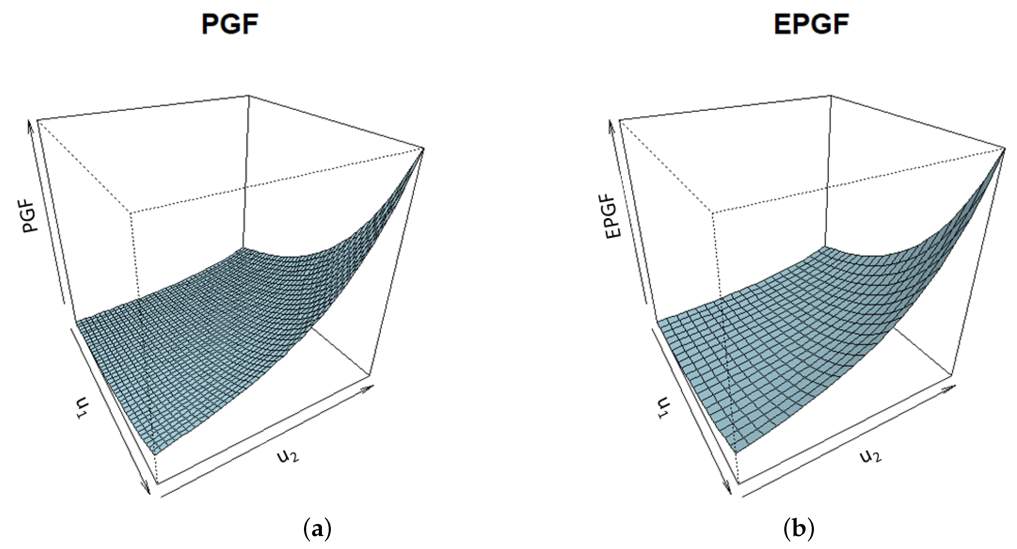
Remark 5.

Using similar considerations as in ECF estimation theory (see, e.g., Yu [31]), the PGF estimators of the (true) parameter $\theta ={\theta }_0$ can be calculated using the realization of a two-dimensional random vector ${\mathbf{Y}}_t^{\left(2\right)}:={(Y_t,Y_{t+1})}^{\prime }$. In that case, the objective function $Q_T^{\left(2\right)}$ is given as a double integral that can be approximately calculated by applying some well-known cubature formulas (see the next section, Section 5). To this end, the two-dimensional PGF of the basic INSB(1) series $\left(Y_t\right)$ should be determined. By replacing $r=2$ in Equation (14) and using Equation (13), this PGF can be obtained in the following way:

$$\begin{array}{cc}\hfill G_Y^{\left(2\right)}(u_1,u_2;\theta )& =\prod _{k=1}^{\infty }\left[1+{\mu }_q\left(\frac{f\left(a(1+{\alpha }^k(u-1))\right)}{f\left(a\right)}-1\right)\right]\hfill \\ \hfill & \times \frac{\left[(1-{\mu }_q)f\left(a{u}_1\right)+{\mu }_{q}f\left(au\right)\right]f\left(a{u}_2\right)}{{\left(f\left(a\right)\right)}^2},\hfill \end{array}$$

(36)

where $u=u_1\left(1+\alpha (u_2-1)\right).$ Figure 2 shows, as an illustration, the theoretical and empirical PGFs of the series $\left(Y_t\right)$ with geometrically distributed PS innovations.

5. Numerical Simulations

In this part, numerical simulations of the PGF estimation procedure for the unknown parameters $\theta ={(a,\alpha ,{\mu }_q)}^{\prime }$ of the INSB(1) process were performed. To that aim, as mentioned earlier, different PS-distributed innovations $\left({\epsilon }_t\right)$ can be considered. For some practical reasons, related to the application of the INAR(1) process that will be further explained, two different PS-distributions of the innovations $\left({\epsilon }_t\right)$ were examined, one with a Poisson distribution and the other with a geometric distribution. Using Monte Carlo simulations, samples of length $T=1000$ were generated in both cases, based on 500 independent realizations of the PS series $\left({\epsilon }_t\right)$. According to that, by applying Equations (3) and (5), respectively, the series of martingale means $\left(X_t\right)$ and the basic INSB series $\left(Y_t\right)$ were then generated. In that way, the realizations $\{Y_1,\dots ,Y_T\}$ of the INSB-based series $\left(Y_t\right)$ were obtained, on which the PGF method could be applied.

The estimators of parameters $\theta ={(a,\alpha ,{\mu }_q)}^{\prime }$ were calculated by minimizing the double integral

$$Q_T^{\left(2\right)}\left(\theta \right)={\int }_{-1}^1{\int }_{-1}^{1}w(u_1,u_2){\left(G_Y^{\left(2\right)}(u_1,u_2;\theta )-{\tilde{G}}_T^{\left(2\right)}(u_1,u_2)\right)}^2\mathrm{d}{u}_1\mathrm{d}{u}_2,$$

(37)

where $w:{[-1,1]}^2\to {\mathbb{R}}^{+}$ is the weight function, and $G_Y^{\left(2\right)}(u_1,u_2;\theta )$ is the two-dimensional PGF of the INSB(1) series $\left(Y_t\right)$. For some specific PS-distributed innovations, this PGF can be obtained after some computation, by using Equation (36). In that way, for PS innovations with Poisson distribution, one obtains

$$\begin{array}{cc}\hfill G_Y^{\left(2\right)}(u_1,u_2;\theta )& =\prod _{k=1}^{\infty }\left[1+{\mu }_q\left(exp\left({\alpha }^k(u-1)a\right)-1\right)\right]exp\left((u_1+u_2-2)a\right)\hfill \\ \hfill & \times \left[1+{\mu }_q\left(exp\left(\alpha u_1(u_2-1)a\right)-1\right)\right],\hfill \end{array}$$

while for PS innovations with geometric distribution, it follows that

$$\begin{array}{cc}\hfill G_Y^{\left(2\right)}(u_1,u_2;\theta )& =\prod _{k=1}^{\infty }\left[1+\frac{{\mu }_q{\alpha }^k(u-1)a}{1-\left(1+{\alpha }^k(u-1)\right)a}\right]·\frac{{(1-a)}^2\left(1-a\left({\mu }_q{u}_1+(1-{\mu }_q)u\right)\right)}{(1-a{u}_1)(1-a{u}_2)(1-au)},\hfill \end{array}$$

where $u=u_1\left(1+\alpha (u_2-1)\right).$ It is worth mentioning that these PGFs are not obtained in closed form, but they can be easily approximated by finite k-terminal products and with arbitrary precision.

After that, the integral in Equation (37) is approximately calculated using the cubature formula:

$$I(h;w):={\int }_{-1}^1{\int }_{-1}^{1}w(u_1,u_2)h(u_1,u_2)d{u}_{1}d{u}_2\approx \sum _{j=1}^N{w}_{j}h(u_{1j},u_{2j}),$$

where $(u_{1j},u_{2j})$ are the cubature nodes and $w_j$ are the weight coefficients. In this case, the Gaussian cubature formulas with $N=36$ nodes were used, where two-dimensional weights are based on the Gegenbauer orthogonal polynomials, i.e.,

$$w_k(u_1,u_2)={\left((1-u_1^2)(1-u_2^2)\right)}^{(k-1)/2},$$

where $k=0,1,2$. Obviously, these cubatures reduce to the well-known Gauss–Chebyshev cubatures of the first type (when $k=0$), Gauss–Chebyshev cubatures of the second type (when $k=2$) and Gauss–Legendre cubatures (when $k=1$). These cubatures were calculated within software package “Orthogonal polynomials” in Wolfram Mathematica language, authorized by Cvetković and Milovanović [34]. Thereafter, minimization of the objective function given by Equation (37) was performed using the box-constrained optimization procedure “nlminb” [35] in the statistical programming language R. At the same time, realizations of a uniform distribution $\mathcal{U}(0,1)$ were taken as the initial values of the parameters.

Table 2. The summary statistics, estimation errors and AN testing of parameter estimates of INSB$\left(1\right)$ process (true parameters are $a=\alpha =0.5$, $c=1$).

Sample		Poisson $({\mathit{\mu }}_{\mathit{q}}\approx 0.3935)$			${\mathit{S}}_{\mathit{T}}^{\left(\mathbf{2}\right)}$	Geometric $({\mathit{\mu }}_{\mathit{q}}=0.5)$			${\mathit{S}}_{\mathit{T}}^{\left(\mathbf{2}\right)}$
		$\widehat{\mathit{a}}$	$\widehat{\mathit{\alpha }}$	${\widehat{\mathit{\mu }}}_{\mathit{q}}$		$\widehat{\mathit{a}}$	$\widehat{\mathit{\alpha }}$	${\widehat{\mathit{\mu }}}_{\mathit{q}}$
$w_0(u_1,u_2)$	Min.	0.3904	0.4358	0.3677	$3.14\times {10}^{-4}$	0.3898	0.4397	0.3950	$3.45\times {10}^{-4}$
	Mean	0.5105	0.4989	0.3897	$9.69\times {10}^{-3}$	0.5082	0.5019	0.4997	$3.62\times {10}^{-3}$
	Max.	0.7619	0.5499	0.4361	$3.05\times {10}^{-2}$	0.7142	0.5760	0.6197	$1.33\times {10}^{-2}$
	MSEE	$4.54\times {10}^{-3}$	$2.77\times {10}^{-3}$	$1.09\times {10}^{-4}$	–	$1.99\times {10}^{-3}$	$2.27\times {10}^{-4}$	$1.18\times {10}^{-4}$	–
	$AD$	0.5576	0.3708	0.8099	–	0.7178	0.2457	0.5065	–
	(p-value)	(0.1303)	(0.3892)	(0.0337 *)	–	(0.0593)	(0.7524)	(0.1967)	–
$w_1(u_1,u_2)$	Min.	0.3836	0.4523	0.3559	$1.59\times {10}^{-4}$	0.3904	0.4255	0.4056	$1.55\times {10}^{-4}$
	Mean	0.5091	0.5002	0.3905	$1.41\times {10}^{-2}$	0.5091	0.5018	0.5016	$1.15\times {10}^{-3}$
	Max.	0.7421	0.5493	0.4234	$4.18\times {10}^{-2}$	0.6832	0.5694	0.5913	$8.01\times {10}^{-3}$
	MSEE	$2.27\times {10}^{-3}$	$7.65\times {10}^{-4}$	$1.02\times {10}^{-4}$	–	$2.06\times {10}^{-3}$	$2.06\times {10}^{-4}$	$1.17\times {10}^{-4}$	–
	$AD$	0.2437	0.2861	0.3188	–	0.5911	0.2410	0.5262	–
	(p-value)	(0.7589)	(0.6178)	(0.5301)	–	(0.1191)	(0.7613)	(0.1714)	–
$w_2(u_1,u_2)$	Min.	0.3951	0.4765	0.3807	$1.12\times {10}^{-4}$	0.4065	0.4175	0.4070	$2.38\times {10}^{-4}$
	Mean	0.5068	0.5012	0.3914	$8.98\times {10}^{-3}$	0.5070	0.4987	0.5018	$1.12\times {10}^{-3}$
	Max.	0.7581	0.5471	0.4284	$2.88\times {10}^{-2}$	0.6486	0.5607	0.6179	$6.52\times {10}^{-3}$
	MSEE	$2.57\times {10}^{-3}$	$6.17\times {10}^{-4}$	$3.08\times {10}^{-4}$	–	$1.98\times {10}^{-3}$	$2.09\times {10}^{-4}$	$9.23\times {10}^{-5}$	–
	$AD$	0.2694	0.3384	0.5972	–	0.2123	0.9120	0.3959	–
	(p-value)	(0.6497)	(0.4734)	(0.1182)	–	(0.8513)	(0.0195 *)	(0.3645)	–

* $0.01<p<0.05$.

presents the summary statistics of the thus obtained PGF estimates, that is, their minimums (Min.), mean values (Mean), maximums (Max.), as well as the mean squared estimation errors (MSEEs), for all proposed weights and both innovation distributions considered. Additionally, the values of the objective functions ${\widehat{S}}_T$ are given, as reference errors in the estimation. Regarding to the results presented, it is seen that the PGF procedure provides efficient parameter estimates, with similar properties, for both innovation series $\left({\epsilon }_t\right)$. Notice that slightly smaller estimation errors are observed with weight $w_2(u_1,u_2)$. This is expected, because this weight emphasizes points around the coordinate origin. On the contrary, somewhat larger errors in the estimation are observed with weight $w_0(u_1,u_2)$, which “forces” ends of the interval $[-1,1]$. Finally, when $k=1$, Gauss–Legendre orthogonal polynomials with weight $w_1(u_1,u_2)\equiv 1$ are obtained. Their accuracy is also satisfactory, and due to their simplicity, similarly to what is reported in Stojanović et al. [19,21], they will be used in some practical applications of the PGF method.

In addition, Table 2 contains the AN test results, where Anderson–Darling normality test was performed. The test statistic, denoted as AD, as well as the corresponding p-values, were calculated using the procedure from the software package “nortest” [36], within the statistical programming language R (version 4.3.2). According to the values thus obtained, it is easy to see that the property of AN is verified for most PGF estimates of parameters $\theta ={(a,\alpha ,{\mu }_q)}^{\prime }$, at the significance level of $0.01<p<0.05$. At the same time, it is worth emphasizing that estimates of critical value c can be simply obtained from the estimates of parameter ${\mu }_q$ and the equality

$$c=\underset{x=0,1,\dots }{inf}\left\{F_{\epsilon }\left(x\right)\ge 1-{\mu }_q\right\}.$$

(38)

6. Application of the Model

Some practical applications of the INSB process in real-world data modeling are discussed here, taking two sets of actual data. The first series, named Series A, represents the number of traffic accidents with a fatal outcome in the Republic of Serbia, collected according to the official statistics of the Office for Information Technologies and Egoverment [37], in the period from 1 January 2015 to 31 December 2021. The second one (Series B) represents the number of forest fires in Evros, one of the largest regional units of the Republic of Greece, with data taken from the official website of the Hellenic Fire Service [38], from 1 January 2019 to 31 December 2021. In that way, count time series of lengths $T_1=2541$ and $T_2=1096$, respectively, were obtained, and their dynamics are shown in Figure 3.

Summary statistics of both series are shown in

Table 3. The summary statistics, stationarity testing and the correlation structure of real-world data.

Statistics	Series A	Series B
Minimum	0	0
Maximum	7	18
Mode	0	0
Median	1	0
Mean	1.261	1.116
St. deviation	1.256	1.763
Variance	1.577	3.109
Skewness	1.062	2.931
Kurtosis	4.099	14.44
ADF-test	−7.705	−5.667
(p-value)	(<0.01)	(<0.01)
ACF(1)	0.150	0.535
ACF(2)	0.119	0.427
⋯	⋯	⋯
ACF(10)	0.115	0.255
⋯	⋯	⋯
ACF(40)	0.083	0.007

, where their specific descriptive characteristics can already be observed. For instance, with Series A, a slight over-dispersion is noticeable. Using the previous theoretical results, it appears that its dynamics can be modeled by an INSB(1) process with Poisson-distributed innovations $\left({\epsilon }_t\right)$. Namely, in this case, $g\left(a\right)=lnf\left(a\right)=a$ holds, and according to Equation (15) in Theorem 2, the over-dispersion index is $D_Y\left(a\right):={\sigma }_Y^2-{\mu }_Y={\alpha }^2{a}^2{\mu }_q{F}_{\epsilon }\left(c\right)/(1-{\alpha }^2)>0.$ On the other hand, when Series B is observed, it is noticeable that the over-dispersion is much more pronounced, as are the properties of zero inflation. Thus, it appears that geometrically distributed PS innovations can be used to model its dynamics.

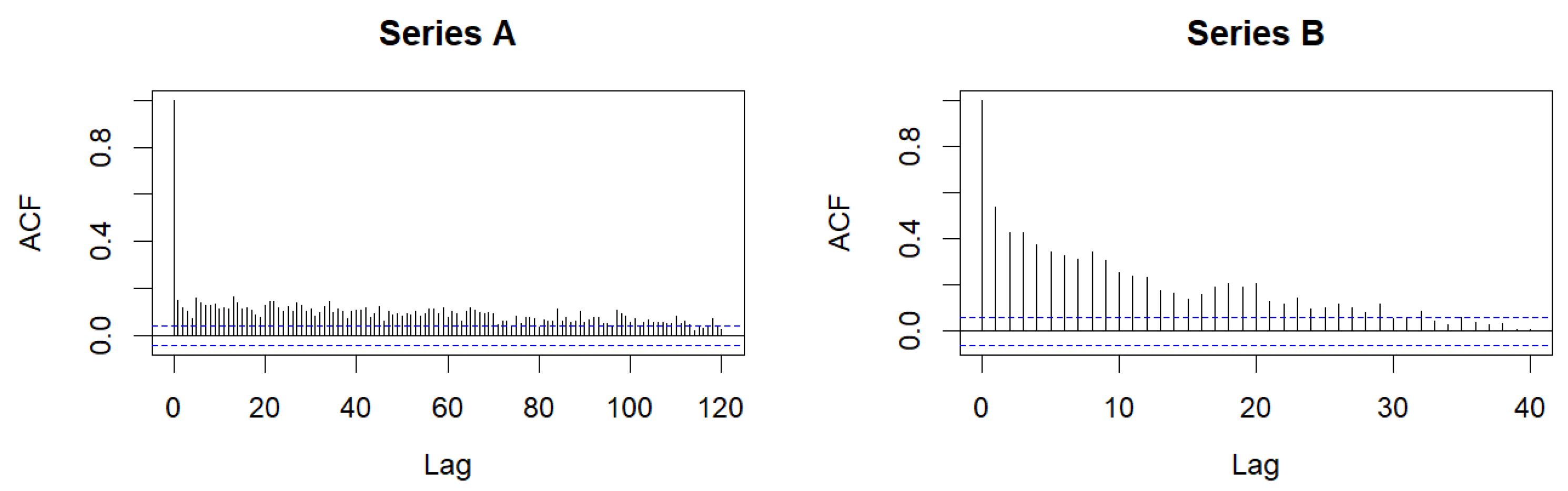
Further, the augmented Dickey–Fuller (ADF) test was conducted, with the alternative hypothesis that the observed series are stationary, which was confirmed in both cases. Also, the estimated values of the autocorrelation functions (ACFs) of both series are decreasing, as is shown in Figure 4. In addition, it is noticeable that the decrease in both ACFs, especially for Series A, is slower than in the case of the regular INAR(1) process. In accordance with previous theoretical results, primarily Theorem 2, this suggests the possibility of modeling the dynamics of both series with the INSB(1) procedure.

On the other hand, the weak correlation in Series A indicates the possibility that the hypothesis of the absence of correlation in the members of this time series is valid here. Therefore, the following null hypotheses are tested here:

$$\begin{array}{cc}\hfill H_0:{\rho }_x\left(k\right)=0\mathrm{and}{\rho }_{\left|x\right|}\left(k\right)=0,& \mathrm{at} \mathrm{individual} \mathrm{lag}k\ge 1,\hfill \\ \hfill H_0:{\rho }_x\left(k\right)=0\mathrm{and}{\rho }_{\left|x\right|}\left(k\right)=0,& \mathrm{for} \mathrm{cumulative}k=1,\dots ,m,\hfill \end{array}$$

where ${\rho }_x\left(k\right)$ and ${\rho }_{\left|x\right|}\left(k\right)$ are the kth-order correlations of the series $\left(x_t\right)$ and $\left(\right|x_t-\mathrm{E}\left(x_t\right)\left|\right)$, respectively. Using the results given by Dalla et al. [39], the above hypotheses are tested using the robust statistics

$$J_{x;\left|x\right|}\left(k\right)=\frac{n^2}{n-k}\left({\widehat{\rho }}_x\left(k\right)+{\widehat{\rho }}_{\left|x\right|}\left(k\right)\right),C_{x;\left|x\right|}\left(k\right)=\sum _{k=1}^m{J}_{x;\left|x\right|}\left(k\right),$$

where ${\widehat{\rho }}_x\left(k\right)$ and ${\widehat{\rho }}_{\left|x\right|}\left(k\right)$ are estimated kth correlations of the above series, respectively. Alternatively, the absence of correlation in the series $\left(x_t\right)$ and ${(x_t-E\left(x_t\right))}^2$ is also tested, via the hypotheses

$$\begin{array}{cc}\hfill H_0:{\rho }_x\left(k\right)=0\mathrm{and}{\rho }_{x^2}\left(k\right)=0,& \mathrm{at} \mathrm{individual} \mathrm{lag}k\ge 1,\hfill \\ \hfill H_0:{\rho }_x\left(k\right)=0\mathrm{and}{\rho }_{x^2}\left(k\right)=0,& \mathrm{for} \mathrm{cumulative}k=1,\dots ,m,\hfill \end{array}$$

where ${\rho }_x\left(k\right)$ and ${\rho }_{x^2}\left(k\right)$ are the appropriate kth-order correlations. Like previously, the statistics used for testing are

$$J_{x;x^2}\left(k\right)=\frac{n^2}{n-k}\left({\widehat{\rho }}_x\left(k\right)+{\widehat{\rho }}_x^2\left(k\right)\right),C_{x;x^2}\left(k\right)=\sum _{k=1}^m{J}_{x;x^2}\left(k\right).$$

For all the above statistics, the following convergences hold:

$$J_{x;\left|x\right|}\left(k\right),J_{x;x^2}\left(k\right)\stackrel{d}{⟶}{\chi }_2^2,C_{x;\left|x\right|}\left(k\right),C_{x;x^2}\left(k\right)\stackrel{d}{⟶}{\chi }_{2m}^2,$$

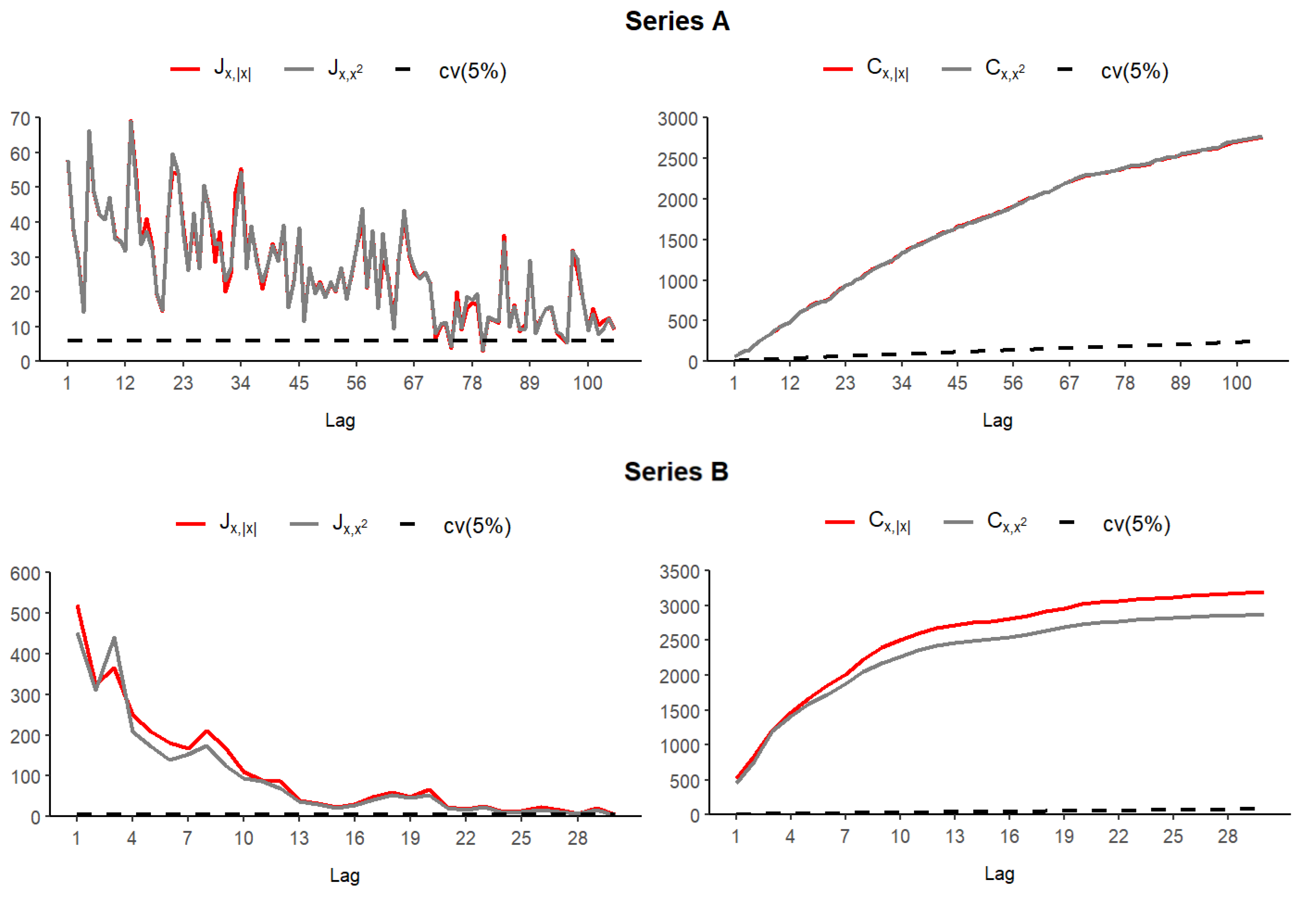
where ${\chi }_2^2$ and ${\chi }_{2m}^2$ are the RVs with chi-square distributions. Figure 5 reports the test results of both observed series, at the significance level $\alpha =5\%$ (showed with dashed lines), obtained using the function “iid.test()“ within the R-package “testcorr“.

In the case of individual testing, it is obvious that the null hypothesis is rejected up to a certain correlation lag. Specifically, with Series A, the i.i.d. property appears for the first time when $k=74$, where the appropriate p-values of the statistics $J_{x;\left|x\right|}\left(k\right)$ and $J_{x;x^2}\left(k\right)$ are equal to 0.144 and 0.114, respectively. Similarly, with Series B, the first i.i.d. case is when $k=30$. On the other hand, following the cumulative tests, it is clear that the null hypothesis of non-correlation of the observed series does not hold at any level. Thus, the assumption about their possible modeling using the INSB(1) process can be justified.

To compare INSB(1) modeling with INAR(1) process modeling, both of these stochastic models were formed based on the observed data. First, by applying equality $Y_t=\alpha \circ Y_{t-1}+{\epsilon }_t,$ where $t=1,2,\dots ,T,$ the INAR(1) model was constructed, whose parameters $(a,\alpha )$ can be estimated using some well-known procedures. Here, the CLS estimation method was applied, based on the minimization of the function

$$\begin{array}{cc}\hfill S_T\left(\theta \right)& :=\sum _{t=2}^T{\left(Y_t-E\left[Y_t|Y_{t-1}\right]\right)}^2=\sum _{t=2}^T{\left(Y_t-\alpha Y_{t-1}-{\mu }_{\epsilon }\right)}^2,\hfill \end{array}$$

(39)

and the CLS-estimates $\tilde{\alpha }$, ${\tilde{\mu }}_{\epsilon }$, same as in the regression procedure, are easily computed by differentiating Equation (39) and equating it to zero. Notice that in the case of the PS distributions family, by using the estimator ${\tilde{\mu }}_{\epsilon }$, estimates of the parameter a can be also easily determined (see, c.f. Table 1). Hence, for the Poisson and geometric distributions, the corresponding estimates are $\tilde{a}={\tilde{\mu }}_{\epsilon }$ and $\tilde{a}={\tilde{\mu }}_{\epsilon }/\left(1+{\tilde{\mu }}_{\epsilon }\right)$, respectively. By applying some basic results of CLS theory [40], the asymptotic properties of the CLS estimators obtained in this way can be proven. The results of this estimation procedure are given in the upper part of

Table 4. Estimated parameters of the INAR(1) and INSB(1) processes, their respective estimation errors and predictive test statistics.

Parameters/Statistics (Stand. Errors)	Series A		Series B
	INAR(1)	INSB(1)	INAR(1)	INSB(1)
a	1.0713 ($5.24\times {10}^{-2}$)	1.0911 ($4.07\times {10}^{-2}$)	0.3422 ($7.79\times {10}^{-3}$)	0.3624 ($7.47\times {10}^{-3}$)
$\alpha$	0.1500 ($2.94\times {10}^{-2}$)	0.1697 ($1.96\times {10}^{-2}$)	0.5348 ($4.26\times {10}^{-3}$)	0.4837 ($4.06\times {10}^{-3}$)
${\mu }_q$	–	0.6290 ($1.96\times {10}^{-2}$)	–	0.4503 ($4.06\times {10}^{-3}$)
$Q_T^{\left(2\right)}$	$1.39\times {10}^{-2}$	$4.63\times {10}^{-3}$	$7.74\times {10}^{-3}$	$3.04\times {10}^{-3}$
MSEE	$1.89\times {10}^{-2}$	$1.82\times {10}^{-2}$	$2.48\times {10}^{-2}$	$1.99\times {10}^{-2}$
AIC	−661.95	−698.43	−531.39	−553.12
$DM$	2.6741 **		2.4683 **
(p-value)	($3.77\times {10}^{-3}$)		($6.86\times {10}^{-3}$)

** $p<0.01$.

.

Taking as initial values the estimates obtained from the previous CLS procedure, the PGF method is then applied. PGF estimates of parameters $\theta ={(a,\alpha ,{\mu }_{\epsilon })}^{\prime }$ are calculated using the previously described estimation procedure, that is, by minimizing the double integral given by Equation (37). In doing so, Gauss–Legendre orthogonal polynomials with weight $w_1(u_1,u_2)\equiv 1$ are used, and the estimated values for both series, along with the corresponding estimated standard errors, are also presented in Table 4. Additionally, parameter estimates of critical value c can be computed using Equation (38), and for Series A and B, these values are $c=0$ and $c=1$, respectively. Accordingly, this means that both series can be equally modeled by the regular INAR(1) or INSB(1) model, although the INSB(1) model appears to have slightly better fitting capabilities.

To confirm this fact, the efficiency of fitting is analyzed for both stochastic models and both of the mentioned estimation procedures. For this purpose, using previously obtained estimated parameter values, 500 Monte Carlo simulations of INAR(1) and INSB(1) time series are generated, while the efficiency of the fit to the real-world data used here is checked using the MSEE statistics and Akaike’s information criterion (AIC). 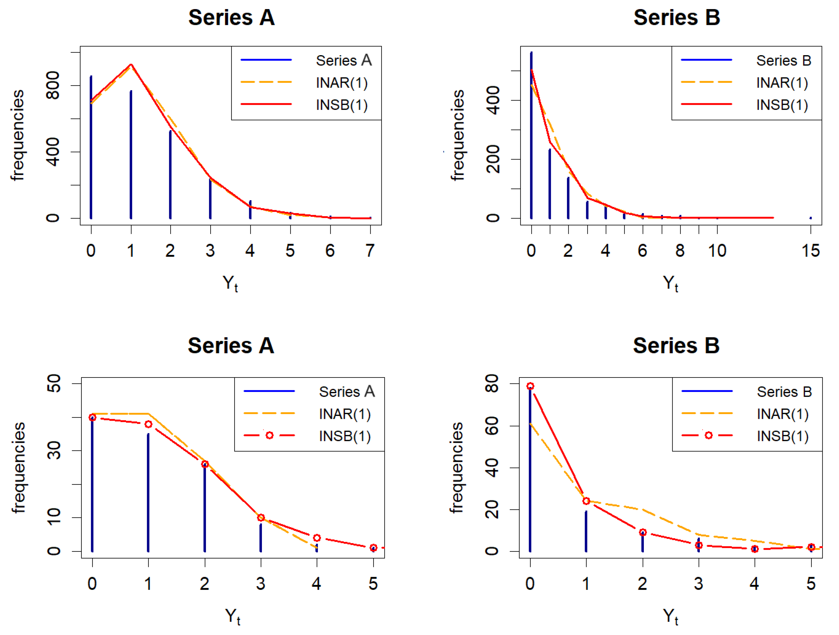Their average values, as well as the values of objective function $Q_T^{\left(2\right)}\left(\theta \right)$, are presented in the middle part of Table 4. It is worth noting that fitting statistics, as well as the estimated parameter values, are close for both series, i.e., for both estimation methods and both stochastic models. However, it is noticeable that the fitting errors are slightly less when the INSB(1) model is applied. This is somewhat more emphasized in the case of Series B, for which it can be concluded that the INSB(1) process represents a more suitable stochastic fitting model. Some of the aforementioned facts can also be observed in the above plots of Figure 4, where the empirical and fitted frequencies of both time series (as well as both stochastic models) are shown.

Finally, for both of these models, the analysis of forecast accuracy based on them is examined. To this end, the time interval from 1 January 2023 to 30 April 2023 was taken as the horizon of the forecast length ($h=120$). The testing procedure was carried out using a one-tailed Diebold–Mariano test of predictive accuracy [41]. More precisely, the null hypothesis was that the INAR(1) and INSB(1) models have the same predictive accuracy, while the alternative hypothesis was that the INSB(1) model has better accuracy. The test statistic, labeled DM, as well as the corresponding p-values, were calculated within the package “forecast” [42] in the statistical programming language R and are presented in the lower part of Table 4. Based on this, it can be seen that the INSB(1) model has better forecast accuracy, which is in accordance with the previous results obtained. As an illustration, the lower diagrams in Figure 6 show the frequency distribution of both models, based on forecast data.

7. Conclusions

A novel count time-series model, named INSB(1) process, is presented here. Using the general form of PS-distributed innovations, as well as the noise indicator series, this stochastic model can be viewed as a generalization of some related models, primarily the INAR(1) processes. The key properties of the proposed model, as well as the procedure for estimating its parameters based on probability-generating functions (PGF method), were discussed in detail. Through Monte Carlo simulations, the consistency of PGF estimators, as well as a practical application of the INSB(1) process in real-world data fitting, was examined. In order to verify the effectiveness of the proposed model, it was applied in fitting distributions and for forecasting two accident-based real-world time series: the number of serious traffic accidents and the number of forest fires. At the same time, the INSB(1) model was also compared with the regular INAR(1) model. Based on the obtained results, that is, the fitting errors and DM-statistics presented in the previous section, the proposed model has the same or even better fitting possibilities with the observed data. According to the above, the better characteristics of the INSB model can be observed, especially in the prediction of future values of the considered time series.

Let us notice that as members of the PS distributions family, two special cases of the INSB(1) model, with Poisson-distributed and geometrically distributed innovations, were considered. For both, the fitting procedures were examined in various aspects, as well as prediction accuracy. The obtained results indicate the appropriateness of the proposed model, which at the same time represents a motivation for further research. This can be conducted, for instance, in defining a higher-order INSB processes or, similar to the General Split-BREAK (GSB) model, to use some other discrete-type stochastic distribution as the innovation series. Finally, it should be mentioned that there are integer-valued distributions that do not belong to the family of PS distributions, which may be a limitation of the proposed model.