Higher-Order INAR Model Based on a Flexible Innovation and Application to COVID-19 and Gold Particles Data

Abstract

INAR models have the great advantage of being able to capture the conditional distribution of a count time series based on their past observations, thus allowing it to be tailored to meet the unique characteristics of count data. This paper reviews the two-parameter Poisson extended exponential (PEE) distribution and its corresponding INAR(1) process. Then the INAR of order p (INAR(p)) model that incorporates PEE innovations is proposed, its statistical properties are presented, and its parameters are estimated using conditional least squares and conditional maximum likelihood estimation methods. Two practical data sets are analyzed and compared with competing INAR models in an effort to gauge the performance of the proposed model. It is found that the proposed model performs better than the competitors.

1. Introduction

Exploring discrete data has become a specialized area in time series analysis, with applications in several industries, including banking, epidemiology, and telecommunications. Integer-valued autoregressive models of order p (INAR(p)) have become effective tools for tackling the complexities of count data. With the help of these models, which reveal the underlying dynamics and temporal connections in discrete time series, phenomena that are measured in discrete units can be understood more precisely.

Count data differ from conventional continuous data in the sense that they have particular difficulties and traits, such as non-negativity and discrete outcomes. Conventional continuous models often struggle to capture the complexities inherent in count-based time series. However, INAR(p) models offer an innovative solution tailored to the distinct properties of count data. The core strength of an INAR(p) model lies in its capacity to capture the conditional distribution of the current count variable, based on its past p observations. This autoregressive framework forms the foundation of the model, allowing it to account for temporal dependencies and seasonality effects commonly found in count time series. As a result, INAR(p) models facilitate accurate forecasting and a deeper comprehension of patterns in discrete data.

In actuality, the INAR(p) model is a development of the INAR(1) model proposed by [1,2]. The initial approach was based on the binomial thinning and Poisson innovations. Considering the fact that count time series are generally overdispersed, the Poisson distribution can no longer be applied to INAR(1). Researchers have proposed various distributions of innovation and thinning operations to overcome this issue. In this context, several researchers have contributed to the study of various models for discrete-valued processes with different modifications. For instance, ref. [3] developed a family of models using Poisson marginal distributions. Subsequently, ref. [4] delved into investigating a novel stationary INAR(1) process with geometric marginal distributions. This was achieved through a negative binomial thinning operator, and they obtained several properties of the process. Ref. [5] introduced another stationary INAR(1) process. In a different work, ref. [6] considered the compound Poisson INAR(1) model, which deals with time series of overdispersed counts. Additionally, ref. [7] investigated first-order non-negative integer-valued autoregressive processes, incorporating power series innovations. Furthermore, ref. [8] constructed an INAR(1) model using Poisson–Lindley distributed innovations. References [9,10,11,12,13], among others, also substantiate this claim.

The studies of [14,15] extended the work of [2] using INAR models with p dependence. Meanwhile, ref. [15] proposed an alternative to the more general INAR(p) process introduced by [14]. According to [15], an INAR(p) process has the same autocorrelation structure as an AR(p), whereas according to [14], it has the same autocorrelation structure as an ARMA($p,p-1$) process. Most authors follow the set-up described by [15]. References [16,17] also contributed to the class of INAR(p) models. Later, ref. [18] introduced an INAR(p) process with a signed generalized power series thinning operator.

Although the INAR(p) model is flexible in dealing with higher-order autoregressive processes, it does not incorporate periodicity, which is a common time series characteristic in a wide range of applications, including air quality and health. Periodically correlated stochastic processes are described in [19] with periodically varying mean, variance and covariance. The flexibility of the seasonal and/or periodic INAR models are studied by [20,21,22,23], among others.

The Poisson extended exponential (PEE) distribution and its related INAR(1) model are discussed in length in [24], and the current study extends that discussion to the INAR(p) model. On the basis of the weekly number of syphilis cases in the United States during 2007–2010, ref. [24] showed that the INAR(1) with PEE innovations performed better than the other competitive INAR(1) models. These findings suggest the need to look at the PEE in other important settings, such as INAR(p) model, and to compare it with other popular INAR(p) models, demonstrating its superiority.

Firstly, in Section 2, we review the PEE distribution and associated INAR(1) model, and then an INAR(p) model based on the PEE distribution is presented, which is named the PEE-INAR(p) model, in Section 3. Section 4 discusses conditional least squares (CLS) estimation, as well as conditional maximum likelihood (CML) estimation. Section 5 provides a simulation study. Section 6 examines how the proposed model works on practical data sets to illustrate its effectiveness. A conclusion is provided in Section 7.

2. The INAR(1) Process with the PEE Innovations

According to [24], a comprehensive definition of the PEE distribution can be found in their paper. Compounding the Poisson and extended exponential (EE) distributions results in the PEE distribution.The probability density function of EE distribution is given by

$$f\left(x\right)=\frac{{\eta }^2(1+\gamma x)e^{-\eta x}}{\eta +\gamma },x>0,\eta >0,\gamma \ge 0.$$

The stochastic structure of a random variable X with a PEE distribution is as follows: If the random variable X follows the PEE distribution, which holds the following stochastic representation, $X|\lambda$∼P$\left(\lambda \right)$ and $\lambda |\eta , \gamma$∼EE$(\eta ,\gamma )$, where $\lambda >0$, $\eta >0$ and $\gamma \ge 0$, then the unconditional probability mass function (pmf) of X has the following form:

$$P(x;\eta ,\gamma )=\frac{{\eta }^2(1+\eta +\gamma +\gamma x)}{(\eta +\gamma ){(\eta +1)}^{x+2}},x=0,1,2,3,....$$

(1)

It is important to note that when $\gamma =1$, (1) is reduced to the discrete Poisson–Lindley distribution (see, ref. [8]). Some of the important properties of the PEE distribution are listed below. The probability generating function for a random variable X with the PEE distribution is provided by

$$G(s;\eta ,\gamma )=\frac{{\eta }^2\left(1-s+\eta +\gamma \right)}{(\eta +\gamma ){(1+\eta -s)}^2},$$

(2)

for $\left|s\right|<\eta +1$. The mean and variance are given by

$$E\left(X\right)=\frac{\eta +2\gamma }{\eta (\eta +\gamma )}$$

and

$$V\left(X\right)=\frac{{\eta }^3+{\eta }^2+4\eta \gamma +3{\eta }^2\gamma +2{\gamma }^2+2\eta {\gamma }^2}{{\eta }^2{(\eta +\gamma )}^2},$$

respectively. The dispersion index (DI) of the PEE distribution is given by

$$\begin{array}{cc}\hfill DI& =\frac{V\left(X\right)}{E\left(X\right)}\hfill \\ \hfill & =1+\frac{{\eta }^2+4\eta \gamma +2{\gamma }^2}{\eta (\eta +\gamma )(\eta +2\gamma )}.\hfill \end{array}$$

In the PEE distribution, DI is always greater than one, demonstrating an overdispersion feature, as $\eta >0, \gamma \ge 0$. PEE distribution is effective as an innovation distribution in INAR(1) process based on binomial thinning, resulting in the PEE-INAR(1) model, ref. [24].

The PEE-INAR(1) Model

The PEE-INAR(1) process is given by

$$X_t=\alpha \circ X_{t-1}+{ϵ}_t,t\in \mathbb{Z},$$

(3)

where $0<\alpha <1$ and the innovation process is denoted by ${\left\{{ϵ}_t\right\}}_{t\in \mathbb{Z}},$ which are independent and identically distributed (iid) integer-valued random variables having mean $E\left({ϵ}_t\right)={\mu }_{ϵ}$ and variance $V\left({ϵ}_t\right)={\sigma }_{ϵ}^2.$ The binomial thinning operator is denoted by the symbol ∘ and is defined as

$$\alpha \circ X_{t-1}:=\sum _{j=1}^{X_{t-1}}{U}_j,$$

(4)

where ${\left\{U_j\right\}}_{j\ge 1}$ is the sequence of Bernoulli random variables called counting series with probability

$$\alpha =Pr(U_j=1)=1-Pr(U_j=0).$$

It is important to note that in (4), these sequences ${\left\{U_j\right\}}_{j\ge 1}$ are independent of each other and of $\left\{{ϵ}_t\right\}$. For the PEE-INAR(1) process, the one step transition probability is given by

$$\begin{array}{cc}\hfill Pr\left(X_t=x_t|X_{t-1}=x_{t-1}\right)& =P(\alpha \circ X_{t-1}+{ϵ}_t=x_t|X_{t-1}=x_{t-1})\hfill \\ \hfill & =\sum _{i=0}^{min(x_t,x_{t-1})}P(\alpha \circ X_{t-1}=i|X_{t-1}=x_{t-1})Pr({ϵ}_t=x_t-i)\hfill \\ \hfill & =\sum _{i=0}^{min(x_t,x_{t-1})}\left(\genfrac{}{}{0pt}{}{x_{t-1}}{i}\right){\alpha }^i{(1-\alpha )}^{x_{t-1}-i}\frac{{\eta }^2(1+\eta +\gamma +\gamma (x_t-i))}{(\eta +\gamma ){(\eta +1)}^{(x_t-i)+2}},\hfill \end{array}$$

where $0<\alpha <1.$ Ref. [25] provides the mean, variance and DI of ${\left\{X_t\right\}}_{t\in \mathbb{Z}}$ by using the mean, variance and DI of the innovation distribution. For the PEE-INAR(1) process, they are

$$E\left(X_t\right)=\frac{\eta +2\gamma }{\eta (\eta +\gamma )(1-\alpha )},$$

$$Var\left(X_t\right)=\frac{{\eta }^2(\eta +\eta \alpha +1)+2{\gamma }^2(\eta +\eta \alpha +1)+\eta \gamma (3\eta (\alpha +1)+4)}{{\eta }^2\left(1-{\alpha }^2\right){(\eta +\gamma )}^2}$$

and

$$DI\left(X_t\right)=\left(1+\frac{1}{(\eta +\gamma )(\alpha +1)}-\frac{1}{(\eta +2\gamma )(\alpha +1)}+\frac{1}{\eta (\alpha +1)}\right).$$

According to [25,26], the conditional expectation, conditional variance, covariance and correlation of the PEE-INAR(1) process are given by

$$E\left(X_t\right|X_{t-1})=\alpha X_{t-1}+\frac{\eta +2\gamma }{\eta (\eta +\gamma )},$$

$$Var\left(X_t\right|X_{t-1})=\alpha (1-\alpha )X_{t-1}+\frac{{\eta }^3+{\eta }^2+4\eta \gamma +3{\eta }^2\gamma +2{\gamma }^2+2\eta {\gamma }^2}{{\eta }^2{(\eta +\gamma )}^2},$$

$$Cov(X_{t+h},X_t)={\alpha }^{h}Var\left(X_t\right)$$

and

$$Cor(X_t,X_{t-h})={\alpha }^h.$$

3. The INAR(p) Model with PEE Innovations

The INAR(1) process in (3) can be extended to the general INAR(p) process to yield

$$X_t={\alpha }_1\circ X_{t-1}+....+{\alpha }_p\circ X_{t-p}+{ϵ}_t,p=1,2,3,\dots ,t\ge p.$$

(5)

where ${ϵ}_t\sim PEE(\eta ,\gamma )$, $0<{\alpha }_m<1, m=1,2,\dots ,p$. Like (3), $\left\{U_{j,m}\right\}$ is made up of independently distributed Bernoulli random variables with the value ${\alpha }_m$. Additionally, ${ϵ}_t$ is supposed to be independent of ${\left\{X_s\right\}}_{s<t}$ at every time. According to [15], if ${\sum }_{m=1}^p{\alpha }_m<1$, then a unique stationary and ergodic solution exists for $\left\{X_t\right\}$. Also, under stationarity, $Cov(X_t,X_{t+h})={\varphi }_{h,t}={\varphi }_h$.

From [27], for the PEE-INAR(p) process, the p-step transition probabilities are given by

$$\begin{array}{c}{\displaystyle P\left(X_t=x_t|X_{t-1}=x_{t-1},X_{t-2}=x_{t-2},\dots ,X_{t-p}=x_{t-p}\right)}\hfill \\ =\sum _{i_1=0}^{min(x_t,x_{t-1})}\left(\genfrac{}{}{0pt}{}{x_{t-1}}{i_1}\right){\alpha }_1^{i_1}{(1-{\alpha }_1)}^{x_{t-1}-i_1}\times \sum _{i_2=0}^{min(x_t-i_1,x_{t-2})}\left(\genfrac{}{}{0pt}{}{x_{t-2}}{i_2}\right){\alpha }_2^{i_2}{(1-{\alpha }_2)}^{x_{t-2}-i_2}\hfill \\ \times \dots \times \sum _{i_p=0}^{min(x_t-(i_1+\dots +i_{p-1}),x_{t-p})}\left(\genfrac{}{}{0pt}{}{x_{t-2}}{i_p}\right){\alpha }_p^{i_p}{(1-{\alpha }_p)}^{x_{t-p}-i_p}P({ϵ}_t=x_t-(i_1+\dots +i_p)).\hfill \end{array}$$

By substituting $P({ϵ}_t=x_t-(i_1+\dots +i_p))$, we get

$$\begin{array}{c}{\displaystyle P\left(X_t=x_t|X_{t-1}=x_{t-1},X_{t-2}=x_{t-2},\dots ,X_{t-p}=x_{t-p}\right)}\hfill \\ =\sum _{i_1=0}^{min(x_t,x_{t-1})}\left(\genfrac{}{}{0pt}{}{x_{t-1}}{i_1}\right){\alpha }_1^{i_1}{(1-{\alpha }_1)}^{x_{t-1}-i_1}\times \sum _{i_2=0}^{min(x_t-i_1,x_{t-2})}\left(\genfrac{}{}{0pt}{}{x_{t-2}}{i_2}\right){\alpha }_2^{i_2}{(1-{\alpha }_2)}^{x_{t-2}-i_2}\hfill \\ \times \dots \times \sum _{i_p=0}^{min(x_t-(i_1+\dots +i_{p-1}),x_{t-p})}\left(\genfrac{}{}{0pt}{}{x_{t-2}}{i_p}\right){\alpha }_p^{i_p}{(1-{\alpha }_p)}^{x_{t-p}-i_p}\frac{{\eta }^2(1+\eta +\gamma +\gamma (x_t-(i_1+\dots +i_p)))}{(\eta +\gamma ){(\eta +1)}^{(x_t-(i_1+\dots +i_p))+2}}.\hfill \end{array}$$

(6)

From [15,25,27,28], we get the mean and variance of the ${\left\{X_t\right\}}_{t\in \mathbb{Z}}$, respectively, as

$$E\left(X_t\right)=\frac{{\mu }_{ϵ}}{\left(1-{\sum }_{m=1}^p{\alpha }_m\right)}=\frac{\eta +2\gamma }{\eta (\eta +\gamma )\left(1-{\sum }_{m=1}^p{\alpha }_m\right)},$$

(7)

$$Var\left(X_t\right)=\frac{{\sum }_{m=1}^p{\alpha }_m(1-{\alpha }_m)E\left(X_t\right)+2{\sum }_{m=1}^p{\sum }_{m=m^{\prime }}^{p-1}{\alpha }_m{\alpha }_{m^{\prime }}{\varphi }_{m^{\prime }-m}+{\sigma }_{ϵ}^2}{\left(1-{\sum }_{m=1}^p{\alpha }_m^2\right)},$$

(8)

where $Cov(X_{t-m},X_{t-m^{\prime }})={\varphi }_{m^{\prime }-m},$ for lag $|m-m^{\prime }|$. Also,

$$Cov(X_t,X_{t+h})=\sum _{m=1}^p{\alpha }_m{\varphi }_{h-m}.$$

(9)

The conditional moments are given by

$$E\left(X_t|X_{t-1},X_{t-2},\dots ,X_{t-p}\right)=\sum _{m=1}^p{\alpha }_m{X}_{t-m}+{\mu }_{ϵ}$$

(10)

and

$$Var\left(X_t|X_{t-1},X_{t-2},\dots ,X_{t-p}\right)=\sum _{m=1}^p{\alpha }_m(1-{\alpha }_m)X_{t-m}+{\sigma }_{ϵ}^2.$$

(11)

A sample path of the model, for instance, is the simulated paths of the PEE-INAR(2) process given in Figure 1. The simulated sample is considered for $n=400$ with different parameter values. These plots show the stationary and ergodic behavior of the time series data.

4. Estimation

Two different methods of parameter estimation are used here to obtain the unknown parameters of the model.

4.1. Conditional Maximum Likelihood

Let $\theta ={({\alpha }_1,{\alpha }_2,....,{\alpha }_p,\eta ,\gamma )}^T$, then the conditional likelihood function is

$$L\left(\theta \right)=\prod _{t=p+1}^{T}Pr\left(X_t=x_t|X_{t-1}=x_{t-1},X_{t-2}=x_{t-2},\dots ,X_{t-p}=x_{t-p}\right).$$

The log-conditional likelihood function is given by

$$l\left(\theta \right)=logL\left(\theta \right)=\sum _{t=p+1}^{T}logPr\left(X_t=x_t|X_{t-1}=x_{t-1},X_{t-2}=x_{t-2},\dots ,X_{t-p}=x_{t-p}\right),$$

(12)

where $Pr\left(X_t=x_t|X_{t-1}=x_{t-1},X_{t-2}=x_{t-2},\dots ,X_{t-p}=x_{t-p}\right)$ is given by (6). The CML estimators $\widehat{\theta }$ is obtained by maximizing (12).

4.2. Conditional Least Squares

The function below is minimized to obtain the CLS estimators of the parameters of PEE-INAR(p) process:

$$S\left(\theta \right)=\sum _{t=p+1}^T{\left(X_t-\sum _{m=1}^p{\alpha }_m{X}_{t-m}-{\mu }_{ϵ}\right)}^2.$$

A simulation study is used to test the performance of CML and CLS estimators in the next section.

5. Simulation Study

Simulation studies were conducted to evaluate the performance of CML and CLS estimates based on finite samples. We consider five different sample sizes (i.e., 50, 100, 200, 300, 400) with 1000 replications.

Table 1. PEE-INAR(2) Simulation Results.

${\mathit{\alpha }}_1$ = 0.5, ${\mathit{\alpha }}_2$ = 0.3, $\mathit{\eta }$ = 1.6, $\mathit{\gamma }$ = 0.7
Parameter	n	CML		CLS
		Bias	MSE	Bias	MSE
${\alpha }_1$	50	−0.00472	0.01616	−0.05084	0.02531
	100	−0.00314	0.00689	−0.02297	0.01125
	200	−0.00184	0.00355	−0.01150	0.00573
	300	−0.00125	0.00226	−0.00937	0.00369
	400	−0.00010	0.00181	−0.00432	0.00280
${\alpha }_2$	50	−0.01962	0.01838	−0.05369	0.02129
	100	−0.01627	0.00868	−0.03749	0.01076
	200	−0.00625	0.00416	−0.01619	0.00571
	300	−0.00504	0.00268	−0.01262	0.00362
	400	−0.00438	0.00208	−0.01032	0.00287
$\eta$	50	−0.09165	0.35569	−0.20154	0.37458
	100	−0.08853	0.18334	−0.14256	0.28982
	200	−0.07156	0.10112	−0.13650	0.14152
	300	−0.06249	0.08055	−0.11754	0.10136
	400	−0.02908	0.06195	−0.06508	0.09931
$\gamma$	50	0.19165	0.15335	−0.19854	0.16169
	100	0.15675	0.11126	−0.16944	0.15609
	200	0.07935	0.05058	−0.16451	0.15126
	300	0.06627	0.05003	−0.13749	0.14404
	400	0.05120	0.03762	−0.08557	0.11326

and

Table 2. PEE-INAR(2) Simulation Results.

${\mathit{\alpha }}_1$ = 0.4, ${\mathit{\alpha }}_2$ = 0.2, $\mathit{\eta }$ = 1.2, $\mathit{\gamma }$ = 0.9
Parameter	n	CML		CLS
		Bias	MSE	Bias	MSE
${\alpha }_1$	50	0.00543	0.01301	−0.04288	0.02287
	100	0.00470	0.00724	−0.01902	0.01254
	200	0.00072	0.00322	−0.01243	0.00567
	300	0.00234	0.00229	−0.00677	0.00410
	400	0.00113	0.00165	−0.00652	0.00286
${\alpha }_2$	50	−0.01558	0.01382	−0.04464	0.01667
	100	−0.00969	0.00820	−0.02861	0.01087
	200	−0.00204	0.00374	−0.01393	0.00536
	300	−0.00337	0.00251	−0.01279	0.00364
	400	−0.00143	0.00189	−0.00873	0.00265
$\eta$	50	−0.04760	0.11652	−0.08939	0.11574
	100	−0.02667	0.06381	−0.08442	0.06985
	200	−0.00988	0.03173	−0.07852	0.04698
	300	−0.00879	0.01873	−0.07821	0.04034
	400	−0.00591	0.01515	−0.02922	0.03297
$\gamma$	50	−0.24843	0.25267	0.27138	0.37775
	100	−0.23901	0.24417	0.25147	0.30304
	200	−0.23631	0.24380	0.24401	0.25091
	300	−0.23352	0.22876	0.24300	0.23349
	400	−0.19476	0.22753	0.23390	0.23187

present the simulation results. Based on this simulation, we can see that the bias and MSE decrease with increasing sample size when using the PEE-INAR(2) model as a higher order of the PEE-INAR(p) model. The parameter combinations are (${\alpha }_1$ = 0.5, ${\alpha }_2$ = 0.3, $\eta$ = 1.6, $\gamma$ = 0.7) and (${\alpha }_1$ = 0.4, ${\alpha }_2$ = 0.2, $\eta$ = 1.2, $\gamma$ = 0.9). Even though their behaviors are similar, the CML often offers less bias and MSE than the CLS, noting that the least bias for negative values is the one with a value close to 0. We have included a condensed version of the underlying R code in Appendix A.

6. Empirical Study

The considered data sets are fitted to INAR(1) and INAR(2) models under different distributed innovations and the model parameters are estimated by the CML method. The following are the competitive models taken for comparison:

(i)

INAR model based on the discrete Teissier innovations (DT-INAR), see [29].

(ii)

INAR model based on the binomial-discrete Poisson Lindley innovations (BDPL-INAR), see [30].

(iii)

INAR model based on the three parameter discrete-Lindley innovations (DLi3-INAR), see [31].

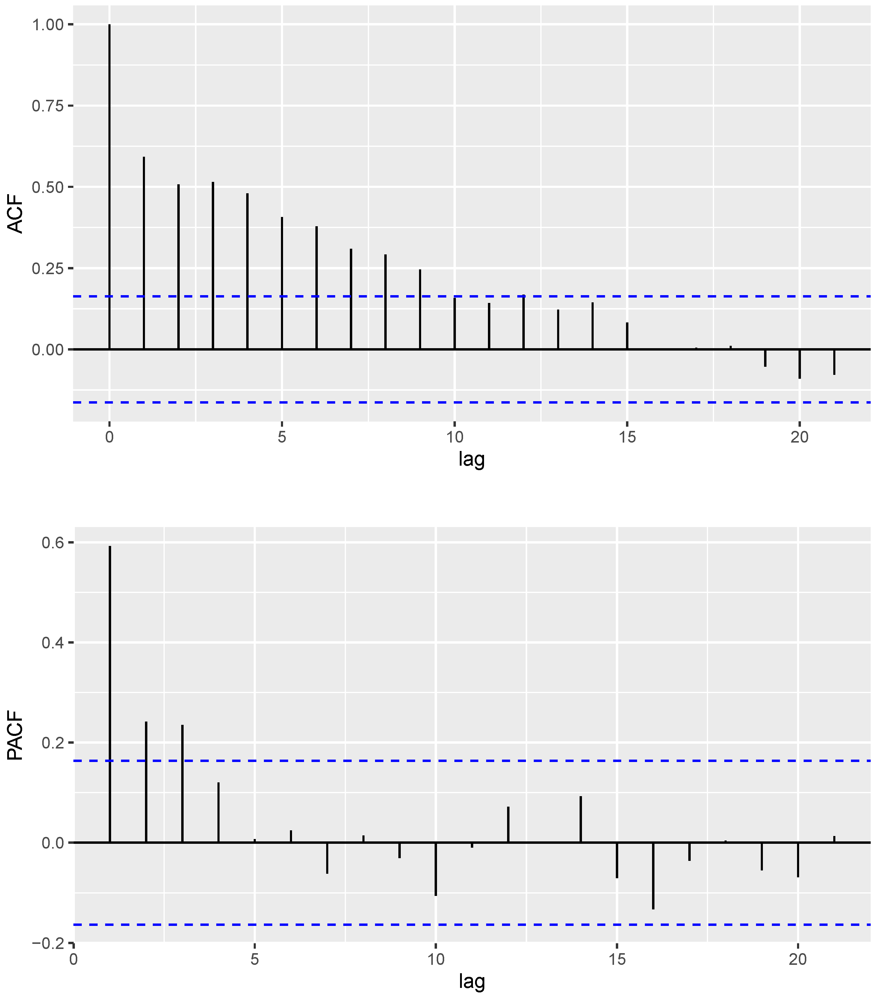
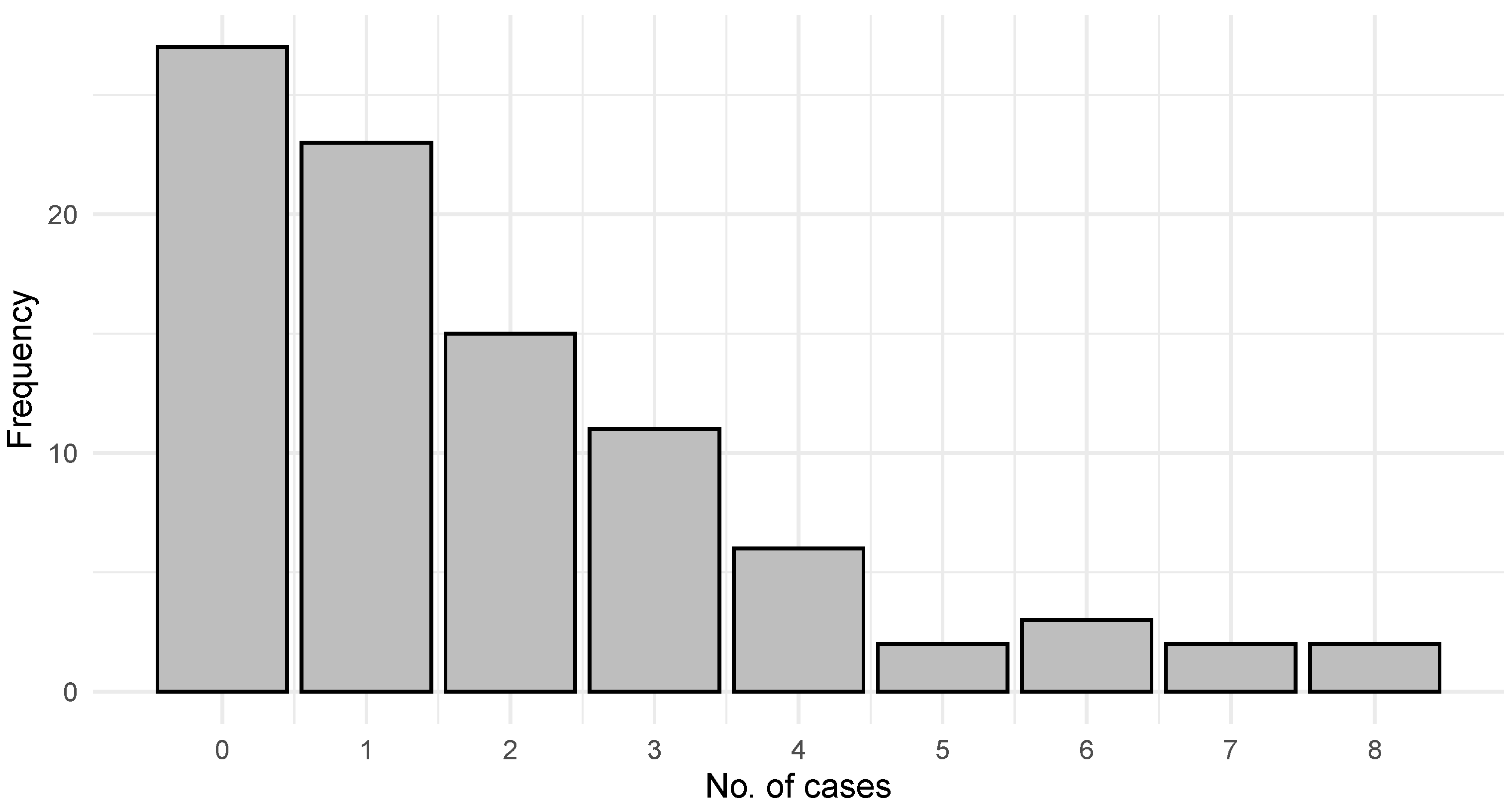
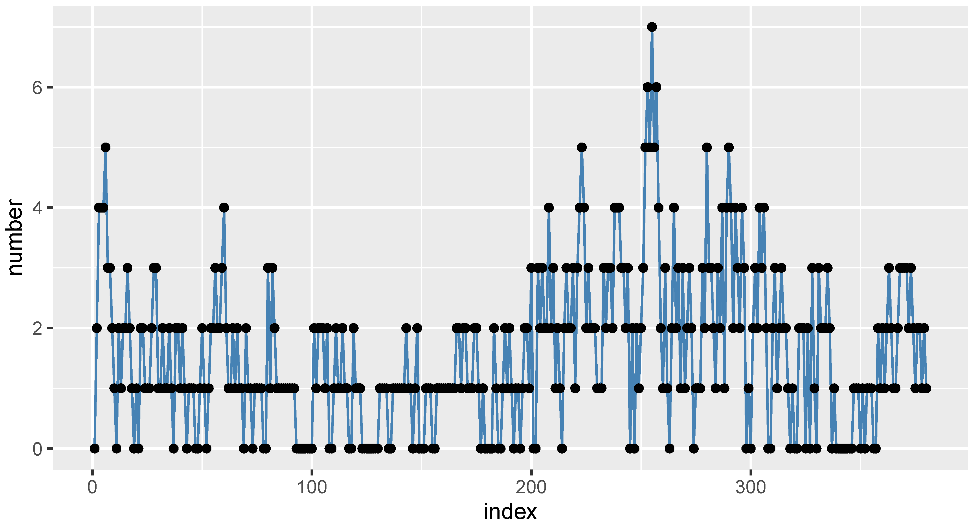
The log-likelihood function, or log L, is calculated for each model, along with Akaike information criterion (AIC) and Bayesian information criterion (BIC) values, which are given as

$$AIC=-2logL+2r$$

and

$$BIC=-2logL+rlogn,$$

where r is the number of parameters. The following is the considered practical data with its analysis.

6.1. COVID-19 Data

Our discussion in this section focuses on the application of the proposed model. A total of 91 observations were gathered about the daily death cases in Switzerland from 1 June 2021 to 30 August 2021. It is taken from the website https://covid19.who.int/data (accessed on 14 September 2023). Accordingly, the mean, variance, and DI are 1.8462, 3.9094 and 2.1175, respectively, which reflects the overdispersion of the data. Figure 2 presents the time series plot of the COVID-19 data. Figure 3 illustrates autocorrelation function (ACF), partial autocorrelation function (PACF) and histogram plots. From the ACF and PACF, it is evident that second-order autoregressive models are the more desirable ones.

Table 3. Fitting results of the COVID-19 data.

Model	Parameter	Estimate	Std Error	log L	AIC	BIC
PEE-INAR(2)	${\alpha }_1$	0.34330	0.08397	−143.33799	294.67599	304.71942
	${\alpha }_2$	0.29190	0.09068
	$\eta$	1.38030	1.42716
	$\gamma$	0.00010	1.39072
PEE-INAR(1)	$\alpha$	0.45897	1.05246	−149.01889	304.03779	311.57037
	$\eta$	1.08045	1.50832
	$\gamma$	0.11301	0.06388
DT-INAR(2)	${\alpha }_1$	0.35590	0.06094	−162.03214	330.06429	337.59686
	${\alpha }_2$	0.27323	0.06300
	$\lambda$	0.48354	0.02498
DT-INAR(1)	$\alpha$	0.40357	0.01799	−181.43955	366.87910	371.90082
	$\lambda$	0.59686	0.05366
BDPL-INAR(2)	${\alpha }_1$	0.34433	0.08350	−143.51806	295.03612	305.07956
	${\alpha }_2$	0.28807	0.09016
	$\lambda$	0.99990	1.91169
	$\beta$	0.48685	1.08893
BDPL-INAR(1)	$\alpha$	0.45899	117.11367	−149.01889	304.03779	311.57037
	$\lambda$	9.53718	116.77791
	$\beta$	8.82505	0.06388
DLi3-INAR(2)	${\alpha }_1$	0.34330	0.08397	−143.33799	296.67599	309.23028
	${\alpha }_2$	0.29190	0.09068
	$\lambda$	6.70660	5.31318
	$\beta$	0.42013	0.25201
	$\theta$	0.00010	3.91858
DLi3-INAR(1)	$\alpha$	0.45926	59.2776	−149.02031	308.04062	320.59491
	$\lambda$	0.6639	3.2197
	$\beta$	0.0352	0.2434
	$\theta$	0.4805	0.0638

presents the data analysis results, which imply that PEE-INAR(2) has the maximum log L and minimum AIC and BIC. Based on the results, the PEE-INAR(2) process provides a better fit than the other competing models.

6.2. Gold Particles Data

The second set of data includes 380 observations, which is taken from [25]. The count values were measured over time in a fixed volume element of a colloidal solution, where the particles move in Brownian motion. In this case, the mean, variance, and DI are, respectively, 1.5605, 1.6242, and 1.0409, which indicates that the data is overdispersed. The time series plot of the gold particles data is illustrated in Figure 4. Figure 5 illustrates the ACF, PACF, and histogram plots. It is evident from the ACF and PACF plots that second-order models are preferred. Data analysis results can be found in

Table 4. Fitting results of the gold particles data.

Model	Parameter	Estimate	Std Error	log L	AIC	BIC
PEE-INAR(2)	${\alpha }_1$	0.49188	0.04530	−522.31596	1052.63192	1068.39260
	${\alpha }_2$	0.20424	0.05276
	$\eta$	4.21543	0.58439
	$\gamma$	9.9990	4.63723
PEE-INAR(1)	$\alpha$	0.57037	0.27852	−534.38144	1074.76288	1086.58339
	$\eta$	2.64733	7.87235
	$\gamma$	9.99000	0.03105
DT-INAR(2)	${\alpha }_1$	0.34821	0.04483	−535.07328	1076.14657	1087.96708
	${\alpha }_2$	0.17003	0.04221
	$\lambda$	0.46375	0.01549
DT-INAR(1)	$\alpha$	0.41251	0.01157	−550.51787	1105.03574	1112.91608
	$\lambda$	0.51266	0.03352
BDPL-INAR(2)	${\alpha }_1$	0.48773	0.04601	−522.46265	1052.92530	1068.68599
	${\alpha }_2$	0.21088	0.05324
	$\lambda$	0.06186	0.06766
	$\beta$	0.01499	0.01673
BDPL-INAR(1)	$\alpha$	0.56887	0.03965	−533.39932	1072.79864	1084.61915
	$\lambda$	0.04884	0.01399
	$\beta$	0.01694	0.03114
DLi3-INAR(2)	${\alpha }_1$	0.49812	0.04445	−524.88199	1059.76397	1079.46483
	${\alpha }_2$	0.22716	0.05073
	$\lambda$	3.87526	2.34043
	$\beta$	0.29820	0.04151
	$\theta$	0.23710	12.46557
DLi3-INAR(1)	$\alpha$	0.54084	3.69433	−530.72820	1071.45641	1091.15726
	$\lambda$	0.00856	719.40720
	$\beta$	1.66825	0.02747
	$\theta$	0.19226	0.03634

, which indicate that the PEE-INAR(2) possesses the maximum log L and minimum AIC and BIC. It appears that the PEE-INAR(2) process provides a better fit than the competing models.

7. Conclusions

The non-negative nature of count data as well as its discrete outcomes make it a unique type of data with specific challenges. It is often difficult for conventional continuous models to capture the complexities of count-based time series. Its core strength lies in its ability to capture the conditional distribution of the current count variable based on its past p observations, which makes INAR(p) models ideal for handling count data that have unique properties. This paper reviews the PEE distribution and INAR(1) process and then proposes the PEE-INAR(p) model. Parameter estimation is based on the CML and CLS methods and various properties of the model are analyzed. Based on the empirical results, it was found that the PEE-INAR(2) model had a better performance in all aspects than all other models compared. In general, the improvement in model fit is attributed to the order of the INAR model or size of the model’s past values (plus the innovation) that it analyzes. In addition, some of the improvement is due to the recommended distribution of innovation, namely the PEE distribution. In summary, the model’s best performance is owing to the data that was chosen using the previously mentioned factors. If the associated bivariate INAR(p) process were built based on the bivariate PEE innovations, the research may take a different direction. It is necessary to modify and study the work substantially in the future, so we will entrust it to future research.

References

1. McKenzie, E. Some simple models for discrete variate time series 1. Jawra J. Am. Water Resour. Assoc. 1985, 21, 645–650. [Google Scholar] [CrossRef]
2. Al-Osh, M.A.; Alzaid, A.A. First-order integer-valued autoregressive (INAR(1)) process. J. Time Ser. Anal. 1987, 8, 261–275. [Google Scholar] [CrossRef]
3. McKenzie, E. Some ARMA models for dependent sequences of Poisson counts. Adv. Appl. Probab. 1988, 20, 822–835. [Google Scholar] [CrossRef]
4. Ristić, M.M.; Bakouch, H.S.; Nastić, A.S. A new geometric first-order integer-valued autoregressive (NGINAR(1)) process. J. Stat. Plan. Inference 2009, 139, 2218–2226. [Google Scholar] [CrossRef]
5. Bakouch, H.S.; Ristić, M.M. Zero truncated Poisson integer-valued AR(1) model. Metrika 2010, 72, 265–280. [Google Scholar] [CrossRef]
6. Schweer, S.; Weiß, C.H. Compound Poisson INAR(1) processes: Stochastic properties and testing for overdispersion. Comput. Stat. Data Anal. 2014, 77, 267–284. [Google Scholar] [CrossRef]
7. Bourguignon, M.; Vasconcellos, K.L. First order non-negative integer valued autoregressive processes with power series innovations. Braz. J. Probab. Stat. 2015, 29, 71–93. [Google Scholar] [CrossRef]
8. Lívio, T.; Khan, N.M.; Bourguignon, M.; Bakouch, H.S. An INAR(1) model with Poisson–Lindley innovations. Econ. Bull. 2018, A, 1505–1513. [Google Scholar]
9. Aghababaei Jazi, M.; Jones, G.; Lai, C.D. Integer valued AR(1) with geometric innovations. J. Iran. Stat. Soc. 2012, 11, 173–190. [Google Scholar]
10. Altun, E.; Bhati, D.; Khan, N.M. A new approach to model the counts of earthquakes: INARPQX(1) process. Appl. Sci. 2021, 3, 274. [Google Scholar] [CrossRef]
11. Altun, E. A new one-parameter discrete distribution with associated regression and integer-valued autoregressive models. Math. Slovaca 2020, 70, 979–994. [Google Scholar] [CrossRef]
12. Popović, P.M. A bivariate INAR(1) model with different thinning parameters. Stat. Pap. 2016, 57, 517–538. [Google Scholar] [CrossRef]
13. Mohammadpour, M.; Bakouch, H.S.; Shirozhan, M. Poisson–Lindley INAR(1) model with applications. Braz. J. Probab. Stat. 2018, 32, 262–280. [Google Scholar] [CrossRef]
14. Alzaid, A.A.; Al-Osh, M. An integer-valued pth-order autoregressive structure (INAR(p)) process. J. Appl. Probab. 1990, 27, 314–324. [Google Scholar] [CrossRef]
15. Du, J.-G.; Li, Y. The integer-valued autoregressive (INAR(p)) model. J. Time Ser. Anal. 1991, 12, 129–142. [Google Scholar]
16. Drost, F.C.; Van Den Akker, R.; Werker, B.J. Local asymptotic normality and efficient estimation for INAR(p) models. J. Time Ser. Anal. 2008, 29, 783–801. [Google Scholar] [CrossRef]
17. Drost, F.C.; Van den Akker, R.; Werker, B.J. Efficient estimation of auto-regression parameters and innovation distributions for semiparametric integer-valued AR(p) models. J. R. Stat. Soc. Ser. Stat. Methodol. 2009, 71, 467–485. [Google Scholar] [CrossRef]
18. Zhang, H.; Wang, D.; Zhu, F. Inference for INAR(p) processes with signed generalized power series thinning operator. J. Stat. Plan. Inference 2010, 140, 667–683. [Google Scholar] [CrossRef]
19. Gladyshev, E.G. Periodically correlated random sequence. Soviet. Math. 1961, 2, 385–388. [Google Scholar]
20. Monteiro, M.; Scotto, M.G.; Pereira, I. Integer-valued autoregressive processes with periodic structure. J. Stat. Plan. Inference 2010, 140, 1529–1541. [Google Scholar] [CrossRef]
21. Buteikis, A.; Leipus, R. An integer-valued autoregressive process for seasonality. J. Stat. Comput. Simul. 2020, 90, 391–411. [Google Scholar] [CrossRef]
22. Liu, Z.; Li, Q.; Zhu, F. Random environment binomial thinning integer-valued autoregressive process with Poisson or geometric marginal. Braz. J. Probab. Stat. 2020, 34, 251–272. [Google Scholar] [CrossRef]
23. Prezotti Filho, P.R.; Reisen, V.A.; Bondon, P.; Ispány, M.; Melo, M.M.; Serpa, F.S. A periodic and seasonal statistical model for non-negative integer-valued time series with an application to dispensed medications in respiratory diseases. Appl. Math. Model. 2021, 96, 545–558. [Google Scholar] [CrossRef]
24. Maya, R.; Chesneau, C.; Krishna, A.; Irshad, M.R. Poisson extended exponential distribution with associated INAR(1) process and applications. Stats 2022, 5, 755–772. [Google Scholar] [CrossRef]
25. Weiß, C.H. An Introduction to Discrete-Valued Time Series; John Wiley & Sons: Hoboken, NJ, USA, 2018. [Google Scholar]
26. Al-Osh, M.; Alzaid, A.A. Integer-valued moving average (INMA) process. Stat. Pap. 1988, 29, 281–300. [Google Scholar] [CrossRef]
27. Bu, R.; McCabe, B.; Hadri, K. Maximum likelihood estimation of higher-order integer-valued autoregressive processes. J. Time Ser. Anal. 2008, 29, 973–994. [Google Scholar] [CrossRef]
28. Joe, H. Likelihood inference for generalized integer autoregressive time series models. Econometrics 2019, 7, 43. [Google Scholar] [CrossRef]
29. Irshad, M.R.; Jodrá, P.; Krishna, A.; Maya, R. On the discrete analogue of the Teissier distribution and its associated INAR(1) process. Math. Comput. Simul. 2023, 214, 227–245. [Google Scholar] [CrossRef]
30. Shirozhan, M.; Okereke, E.W.; Bakouch, H.S.; Chesneau, C. A flexible integer-valued AR(1) process: Estimation, forecasting and modeling COVID-19 data. J. Stat. Comput. Simul. 2023, 93, 1461–1477. [Google Scholar] [CrossRef]
31. Eliwa, M.S.; Altun, E.; El-Dawoody, M.; El-Morshedy, M. A new three-parameter discrete distribution with associated INAR(1) process and applications. IEEE Access 2020, 8, 91150–91162. [Google Scholar] [CrossRef]
Figure 1. The simulated paths of the PEE-INAR(2) process.
Axioms 13 00032 g001aAxioms 13 00032 g001b
Figure 2. The time series plot of the COVID-19 data.
Axioms 13 00032 g002
Figure 3. The ACF, PACF, and histogram plots of the COVID-19 data.
Axioms 13 00032 g003aAxioms 13 00032 g003b
Figure 4. The time series plot of the gold particles data.
Axioms 13 00032 g004
Figure 5. The ACF, PACF, and histogram plots of the gold particles data.
Axioms 13 00032 g005