Abstract
An extension of the Generalized Autoregressive Score (GAS) model is presented for time series with excess null observations to include explanatory variables. An extension of the GAS model proposed by Harvey and Ito is suggested, and it is applied to precipitation data from a city in Chile. It is concluded that the model provides adequate prediction, and furthermore, an analysis of the relationship between the precipitation variable and the explanatory variables is shown. This relationship is compared with the meteorology literature, demonstrating concurrence.
Keywords:
generalized autoregressive score; zero-augmented; generalized beta dynamic conditional score model distribution of the second kind; time series MSC:
62M10
1. Introduction
In recent times, models with varying parameters have gained increasing popularity for working with time-series data. One of these models is the Generalized Autoregressive Score (GAS), or the Dynamic Conditional Score (DCS). According to Creal et al. [1], these models belong to the class of observation-driven models.
Sometimes, a significant proportion of observations in a time series is zeros, while the remaining observations are positive and are measured on a continuous scale. An example of this is daily precipitation, where there are many days with no rainfall, resulting in these days being recorded as zeros. To work with this type of data, it is necessary to utilize the zero-augmented distributions introduced by Hautsch et al. [2]. This approach, developed by Harvey and Ito [3], provides a framework for working with GAS models in the presence of a significant frequency of zeros.
The objective and contribution of this paper is to extend the model proposed in [3] to include explanatory variables. To achieve this, this research is structured as follows: Section 2 briefly introduces the necessary theory for conducting this study and incorporates the explanatory variables. Section 3 presents the obtained results, which are discussed in Section 4. Finally, the conclusions are drawn in Section 5.
2. Materials and Methods
This section provides a summary of the GAS models [1], the zero-augmented distributions [2], and the integration of these concepts. The goal is to subsequently expand the model using explanatory variables.
2.1. GAS Models
GAS models [1], also known as DCS models [4], are observation-driven models. Blasques et al. [5] define these models for an observed time series with a density given by . This density depends on the time-varying parameter , past observations , and static parameters . The time-varying parameter is defined as the function .
An example of the updated equation is , where , is the weighted score, , and .
Since the vector is unknown, it is estimated using the maximum likelihood method, maximizing .
2.2. Zero-Augmented Distribution for Non-Negative Variables
Consider a non-negative continuous random variable X with independent observations . To account for excess zeros, Hautsch et al. [2] allocate a probability mass at the exact zero value and define probabilities and .
Conditional on , X follows a continuous distribution with density , which is continuous for . Consequently, the unconditional distribution of X is semicontinuous with a discontinuity at zero. This implies the density , where , is a point probability mass at , and denotes the indicator function that takes the value 1 for and 0 otherwise. The probability is treated as a parameter of the distribution that determines how much probability mass is assigned to the strictly positive part of X support. In [3], a GAS model using a aero-augmented distribution is presented and applied to precipitation data. In that work, the possibility of extending the model using explanatory variables is raised, which is addressed in this paper.
2.3. Dynamic Model for the Zero-Augmented Distribution Model
To model time series with excess null observations, Harvey and Ito [3] defined a probability density function for which it is possible to identify a scale parameter . In the context of GAS models, it is necessary to use a link function to introduce dynamics to the parameter, making .
According to Harvey and Ito [3], in a parameter-driven model, the dynamics should be introduced through the parameter . Conversely, the DCS model is observation-driven, with the predictive distribution defined conditional on a filtered value of , denoted as .
For an observed time series , let , where is the probability density function of obtained from a zero-augmented distribution. In other words, . Harvey and Ito [3] introduced dynamics to through a logistic transformation, so when depends on , it yields:
Thus, the probability density function associated with takes the form:
2.4. Derivation of the Model’s Score
To obtain the score of the model, (2) is rewritten as follows:
By taking the derivative of the logarithm of (3) with respect to and considering (1), the score of the model is given by:
When expressed in terms of the indicator function , this becomes:
2.5. Generalized Beta Distribution of the Second Kind
For precipitation data, Harvey and Ito [3] recommend using the generalized beta distribution of the second kind [6], which is given by:
where, , with b being the scale parameter, and , and q are the shape parameters. According to Kleiber and Kotz [7], the non-central moments of order are given by:
At the same time, the density of a generalized beta distribution of the second kind exhibits considerable flexibility, as demonstrated in Figure 1.
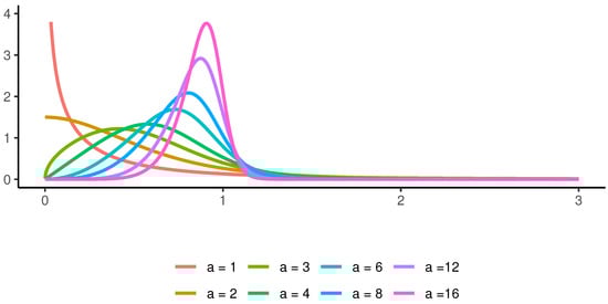
Figure 1.
Generalized beta distribution of the second kind density function for , , .
Special cases encompass a broad range of distributions for non-negative variables. For instance, when , the distribution becomes the Burr distribution, and when , it becomes a log-logistic distribution (McDonald [8]).
2.6. GAS Model for a Zero-Augmented Distribution
We work with the generalized beta distribution of the second kind for which the density is given by (5). Using the exponential link function and incorporating the time dynamics, it yields:
Thus, the model for in terms of the time-varying parameter is:
with a probability density function given by:
where is the density of a generalized beta distribution of the second kind given in (7), , is defined in (1), and
where is the conditional score of the model and is the weight assigned to it.
2.7. Explanatory Variables
In Harvey and Luati [9], it is demonstrated that for a model for which the location parameter denoted by is time-varying, the model depends on a set of explanatory variables denoted by a vector as well as the past values and the score through the following formulation:
where is also a vector representing parameters that are estimated in the model for each explanatory variable.
2.8. Diagnosis
Diebold et al. [10] state that to evaluate whether a model is well-fitted, it should be demonstrated that the probability integral transform (PIT) of
is independent and identically distributed as the uniform distribution , where represents the density forecasts of the generating process .
2.9. Prediction
To obtain predictions, Blasques et al. [5] create confidence bands for the time-varying parameter . They consider the model for an observed time series given by with the update equation
In GAS models, , by construction, depends on , so the parameters need to be obtained from time .
Harvey and Ito [3] accomplish this through computational simulation, following the steps outlined below for :
- (A)
- Given the point estimate by maximum likelihood and the filtered value obtained from (11) for and , simulate S realizations from the estimated conditional density at time . In other words,
- (B)
- Given the simulated observations and equation (11), obtain the filtered values , conditioned on and , using:
- (C)
- For , repeat steps (A) and (B) for the periods .
- (D)
- Use to calculate forecast bands at the desired percentiles.
2.10. Brier Probability Score
To evaluate the quality of the prediction, the Brier probability score (BPS) will be used as a measure of accuracy. This metric is widely employed in such cases (Wilks [11]). BPS was introduced by Brier et al. [12] and is given by:
where n represents the number of predicted values, is the predicted probability at time t, and takes the value 1 if the event occurred at time t and 0 otherwise. Since , Salvador [13] suggests that predictions are acceptable if .
2.11. Application
The zero-augmented GAS model to be formulated will be applied to precipitation data. Let represent the amount of precipitation in period t. Then,
It is assumed that the data-generating process for precipitation follows the zero-augmented generalized beta distribution of the second kind. As a result, the conditional density of is defined as:
where is given in (1), is the density of the generalized beta distribution of the second kind, which, according to Harvey and Ito [3], for improved estimates, should be reparameterized from (7) in terms of the reciprocal of the tail index: , where is the tail index. This leads to:
where are shape parameters, and is the scale parameter modeled through , which acts as the location parameter. Replacing it with in Equations (9) and (10) results in:
where and are parameters to be estimated; , where with are the explanatory variables; , where with are the parameters to be estimated; and is the conditional score of the model, given by:
where is given by Equation (8).
The conditional mean, obtained directly from (6), is given by:
2.12. Dataset
The employed time series corresponds to the daily precipitation in the city of Puerto Montt in Chile, as shown in Figure 2. This variable is measured in millimeters (mm) and is equivalent to the liters of water that have fallen per square meter. The dataset was divided into two parts: the first part was used for model estimation and covers from 1 January 2011 to 31 December 2020 with a total of 3653 observations, out of which 1648 data points are zeros. The second part consisted of the following 244 observations, of which 127 data points were zeros. The data used were obtained from the website of the Dirección Meteorológica de Chile “http://www.meteochile.gob.cl/ (accessed on 22 November 2022)”, and the records belong to the El Tepual Puerto Montt Ap Station (code 410005).
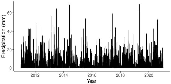
Figure 2.
Precipitation in Puerto Montt, Chile.
As explanatory variables, the following were used: relative humidity, measured in percentage (%); atmospheric pressure, measured in hectopascals (hPa); and temperature, measured in degrees Celsius (°C). The daily maximum values reached by these variables were used.
Figure 3, Figure 4 and Figure 5 present the graphs of the explanatory variables, while Table 1 shows the descriptive statistics of these explanatory variables.
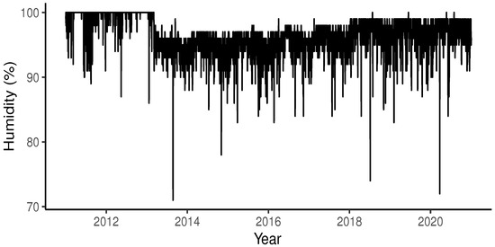
Figure 3.
Humidity in Puerto Montt, Chile.
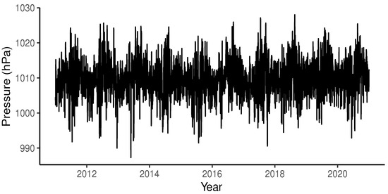
Figure 4.
Pressure in Puerto Montt, Chile.
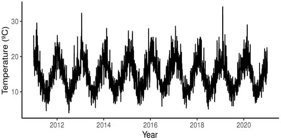
Figure 5.
Temperature in Puerto Montt, Chile.

Table 1.
Descriptive statistics.
2.13. Parameter Estimation
The estimation of the vector was performed using the method of maximum likelihood, formulating the maximization problem as:
The calculations were performed in the R programming language using the GB2 package (Graf et al. [14]), maxLik package (Henningsen and Toome [15]), pracma package (Borchers [16]), and DEoptim package (Mulle et al. [17]).
3. Results
In Table 2, the parameter estimates of the model are presented, along with their statistical significance and standard deviation in parentheses.
Table 2.
Estimated parameters of the model.
Figure 6 presents a graph of the precipitation in Puerto Montt and the adjusted mean.
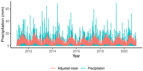
Figure 6.
Fitted model for rainfall in Puerto Montt, Chile.
Figure 7 depicts the empirical cumulative distribution function (ECDF) plotted against transformed integral probabilities for positive observations, while Table 3 displays the result of the Kolmogorov–Smirnov test along with its p-value.
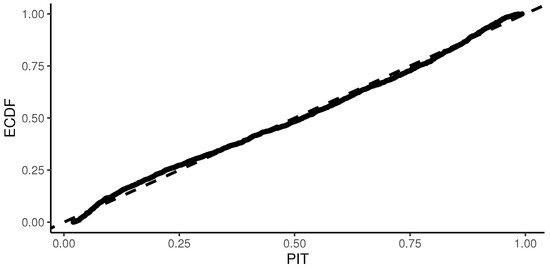
Figure 7.
Probability integral transform (PIT) against the empirical cumulative distribution function (ECDF).
Table 3.
Kolmogorov–Smirnov test results.
The graph for the predicted scale parameter is shown in Figure 8, and Figure 9 displays the graph for the prediction of the conditional mean , as given in (13).
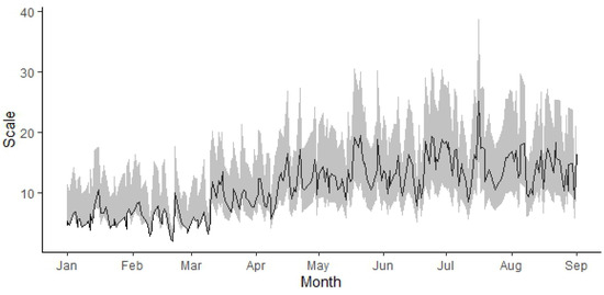
Figure 8.
Prediction of the scale parameter with and the confidence band for each time within the observation period.
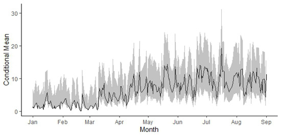
Figure 9.
Prediction of the conditional mean with and its corresponding confidence band for each time within the observation period.
Figure 10 illustrates the predictions for the probability of no rainfall. The shaded regions represent the 95% confidence bands. Notably, .
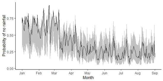
Figure 10.
Prediction of with and the confidence band for each time within the observation period.
4. Discussion
The goodness-of-fit of the model is evident from Figure 6 and is supported by the information in Table 2, where most of the estimated parameters are significant.
Additionally, Figure 7 indicates that the plot of PITs against the ECDF suggests that the data follow the distribution estimated by the model. This alignment is further confirmed by the Kolmogorov–Smirnov test results presented in Table 3, which verify that the model’s PITs follow a uniform distribution .
It is necessary to emphasize that to find out if the PITs had a uniform distribution , two methods were considered:
- (a)
- The classic Kolmogorov–Smirnov test;
- (b)
- A permutation and bootstrap approach. For this, the algorithm described in Præstgaard [18] was implemented, as suggested by one of the reviewers.
Figure 8 illustrates the predictions of the scale parameter of the model, which, combined with the estimated parameter vector , allows for density function forecasts at each prediction time point. Using these density functions (obtained from estimated parameters), conditional means are calculated and presented in Figure 9 as point estimates.
Figure 10 depicts the behavior of the parameter associated with the probability of taking a value of zero in the predictions. These values contribute to calculating the Brier probability score of the model, which has been calculated as , indicating adequate model performance according to Salvador [13].
In Figure 8, Figure 9 and Figure 10, from January to March, it can be observed that the predicted values cluster around one end of the band. This behavior arises from the nature of the zero-augmented distribution model, as explained below:
Initially, in period , the values of the scale and the probability of rainfall need to be determined, yielding and , respectively. As the value of is close to 0, the simulations initially produce many zeros compared to positive values. This phenomenon directly impacts the behavior observed at the lower end of Figure 8 and Figure 9 and at the upper end of Figure 10, as it corresponds to the predictions of .
With the values from the preceding paragraph along with the estimation of , the density presented in Figure 11 is fully determined. Following the procedure outlined by Blasques et al. [5], using this density, values of y are simulated. For this purpose, 1000 simulations were conducted, and the resulting histogram is displayed in Figure 12.
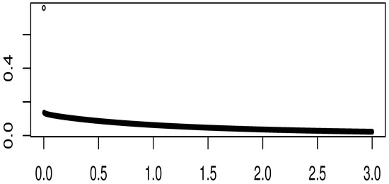
Figure 11.
Probability density function with .

Figure 12.
Simulations of with .
As characteristic of a zero-augmented distribution density, Figure 12 exhibits a high frequency of zeros since the probability of no precipitation is . Therefore, such a proportion of zeros was expected.
With the aforementioned results, the conditional score, , is obtained, as shown in Figure 13. It is noticeable that it inherits the shape of the graph in Figure 11.
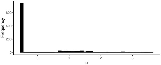
Figure 13.
Simulations of the score with .
Now, it is possible to calculate the scale parameter for time , as depicted in Figure 14, which exhibits a similar pattern to that of Figure 11.
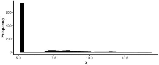
Figure 14.
Scale simulations with .
The same applies to the parameter for the probability of rain for time , which is presented in Figure 15.
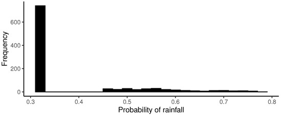
Figure 15.
Simulations of with .
From the histograms of Figure 12, Figure 13, Figure 14, Figure 15, Figure 16 and Figure 17, the high frequency of zeros in the simulated observations causes the calculated values to inherit the same pattern. Therefore, if a specific point prediction is desired, such as the median, for instance, it should be approximated towards the side where the highest frequency lies. As mentioned before, this situation occurs during the period from January to March, which is natural due to it being the summer season in Chile. In other words, the probability of no rainfall is significantly higher compared to the other months. This pattern changes in the following months as the probabilities of no rainfall decrease (see Figure 10), and this is reflected in the corresponding predictions.
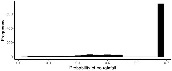
Figure 16.
Simulations of with .
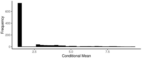
Figure 17.
Simulations of with .
Next, the estimated coefficients of the explanatory variables , , and are interpreted. From (12), it follows that:
Since the scale parameter of the model is
when derived with respect to any of the explanatory variables, with , the result is:
hence, the sign of determines whether increases or decreases. If , then grows, and if , then decreases. Additionally, higher values of the scale parameter result in greater dispersion of the density, while lower values of the scale parameter lead the density to concentrate more around zero. This concentration causes a decrease in the probabilities of high values of the variable, in contrast to when the density becomes more spread out.
Regarding the probability of rain, given in (1), when deriving it with respect to any of the explanatory variables, with , the following is obtained:
As seen in Table 2, where , the sign of determines whether increases or decreases.
Finally, by differentiating the conditional mean, given in (13), with respect to any of the explanatory variables, with , we have:
From this, the sign of determines whether the conditional mean increases or decreases. If , then , , and the derivatives within the last parentheses are positive, and when , the opposite occurs.
In summary, the following cases can be observed:
- (I)
- If , then the scale, , increases, increasing the dispersion for , making higher values more likely. Additionally, the probability of rain, , increases, and the conditional mean, , also increases.
- (II)
- If , then the scale, , decreases, concentrating the density of the distribution around zero for , making higher values less likely. Additionally, the probability of rain, , decreases, and the conditional mean, , also decreases.
Since (see Table 2) and is the coefficient associated with humidity and, according to Llasat Botija et al. [19], humidity promotes the formation of clouds that will lead to rainfall, this aligns with case (I).
On the other hand, (see Table 2), which is the coefficient associated with pressure and corresponds to case (II). According to García de Pedraza [20], when pressure increases, the skies are clearer, a condition that does not favor rainfall. Conversely, if the pressure decreases, it is a condition that favors cloud formation and rain. Therefore, the results align with meteorological science.
Meanwhile, (see Table 2), which is the coefficient associated with temperature and also corresponds to case (II). Regarding this, Trenberth et al. [21] mention that during the warm season over continents, higher temperatures are associated with lower precipitation amounts, while in colder seasons, lower temperatures indicate higher precipitation. Thus, an inverse relationship between temperature and rainfall would exist, but it is more related to the time of year. It is worth noting that this relationship is complex, and exceptions can occur. For example, higher temperatures could also promote cloud formation through water evaporation.
5. Conclusions
A model has been extended for data originating from a zero-augmented distribution: that is, it is to be used in time series where there is a high-frequency proportion of zeros. Additionally, it has been considered that the non-zero data come from a continuous distribution with support for positive values, following the GAS models guidelines of Harvey and Ito [3], as this would not be possible using classical models such as those of Box & Jenkins [22]. This has been applied in meteorology with the precipitation data from a city in Chile. The model has been successfully fitted and responds well to diagnostic tests.
When evaluating the predictive capability of the proposed model, the Brier PS score yielded a value of , categorizing the model as suitable, in contrast to the values presented by Harvey and Ito [3], which were around and . The low value of the Brier PS score for the proposed model could signal that by incorporating explanatory variables, the fit of this type of model can be improved.
Regarding the explanatory variables, it was also very interesting to provide an interpretation of the estimated coefficients associated with each explanatory variable and to confirm that the results of the proposed model, regarding the relationship between precipitation and the explanatory variables humidity, pressure, and temperature, generally align with what is established in meteorology.
It is interesting to analyze how these models behave when the distribution associated with the non-zero part is not necessarily positive and/or continuous. For example, a discrete distribution could be used to analyze time series of the number of COVID-19 fatalities, where there is a high frequency of zeros. This could help determine whether the prediction quality remains consistent under such circumstances.
When it comes to applications in meteorology, it would be compelling to explore how to incorporate explanatory variables related to wind. These variables are known by a specific term in the literature—they are referred to as ’circular data’—and they have a distinctive treatment approach. This aspect has been studied in works by Harvey et al. [23] and Fisher and Lee [24].
It could also be important to analyze the scenario where a specific distribution cannot be identified for the non-zero part. In this case, it could be relevant to explore how to incorporate a more advanced system into these models, such as kernel density estimations for time series. These have also been studied in works such as those by Harvey and Oryshchenko [25] and Harvey [4], where non-parametric statistical tools are used to create distribution-free time-series models.
Author Contributions
Conceptualization, S.C.-E. and P.V.-G.; methodology, F.N.-M.; software, P.V.-G.; validation, S.C.-E., F.N.-M. and P.V.-G.; formal analysis, F.N.-M.; investigation, S.C.-E. and P.V.-G.; resources, F.N.-M.; data curation, P.V.-G.; writing—original draft preparation, F.N.-M.; writing—review and editing, S.C.-E.; visualization, P.V.-G.; supervision, F.N.-M.; project administration, S.C.-E. All authors have read and agreed to the published version of the manuscript.
Funding
Novoa-Muñoz’s research was fully supported by project 2220529 IF/R and Fondo de Apoyo a la Participación a Eventos Internacionales (FAPEI) at Universidad del Bío-Bío, Chile. Contreras-Espinoza was supported by Fondo de Apoyo a la Participación a Eventos Internacionales at Universidad del Bío-Bío, Chile.
Data Availability Statement
The data are obtained from the Meteorological Directorate of Chile “http://www.meteochile.gob.cl/” (accessed on 22 November 2022)—specifically, from “https://climatologia.meteochile.gob.cl/” (accessed on 22 November 2022). And the records belong to the El Tepual Puerto Montt Ap Station (code 410005).
Acknowledgments
The authors would like to thank the anonymous reviewers and the editor of this journal for their valuable time and their careful comments and suggestions because of which the quality of this paper has been improved.
Conflicts of Interest
The authors declare no conflict of interest.
Abbreviations
The following abbreviations are used in this manuscript:
| GAS | Generalized Autoregressive Score |
| DCS | Dynamic Conditional Score |
| BPS | Brier Probability Score |
| ECDF | Empirical Cumulative Distribution Function |
| PIT | Probability Integral Transform |
References
- Creal, D.; Koopman, S.J.; Lucas, A. Generalized autoregressive score models with applications. J. Appl. Econom. 2013, 28, 777–795. [Google Scholar] [CrossRef]
- Hautsch, N.; Malec, P.; Schienle, M. Capturing the zero: A new class of zero-augmented distributions and multiplicative error processes. J. Financ. Econom. 2014, 12, 89–121. [Google Scholar] [CrossRef]
- Harvey, A.; Ito, R. Modeling time series when some observations are zero. J. Econom. 2020, 214, 33–45. [Google Scholar] [CrossRef]
- Harvey, A.C. Dynamic Models for Volatility and Heavy Tails: With Applications to Financial and Economic Time Series; Cambridge University Press: New York, NY, USA, 2013; Volume 52. [Google Scholar]
- Blasques, F.; Koopman, S.J.; Łasak, K.; Lucas, A. In-sample confidence bands and out-of-sample forecast bands for time-varying parameters in observation-driven models. Int. J. Forecast. 2016, 32, 875–887. [Google Scholar] [CrossRef]
- McDonald, J.B.; Xu, Y.J. A generalization of the beta distribution with applications. J. Econom. 1995, 66, 133–152. [Google Scholar] [CrossRef]
- Kleiber, C.; Kotz, S. Statistical Size Distributions in Economics and Actuarial Sciences; John Wiley & Sons: Hoboken, NJ, USA, 2003. [Google Scholar]
- McDonald, J.B. Some generalized functions for the size distribution of income. In Modeling Income Distributions and Lorenz Curves; Springer: New York, NY, USA, 2008; pp. 37–55. [Google Scholar]
- Harvey, A.; Luati, A. Filtering with heavy tails. J. Am. Stat. Assoc. 2014, 109, 1112–1122. [Google Scholar] [CrossRef]
- Diebold, F.X.; Gunther, T.A.; Tay, A.S. Evaluating Density Forecasts with Applications to Financial Risk Management. Int. Econ. Rev. 1998, 39, 863–883. [Google Scholar] [CrossRef]
- Wilks, D.S. Statistical Methods in the Atmospheric Sciences; Academic Press: Cambridge, MA, USA, 2011; Volume 100. [Google Scholar]
- Brier, G.W. Verification of forecasts expressed in terms of probability. Mon. Weather Rev. 1950, 78, 1–3. [Google Scholar] [CrossRef]
- Salvador, J.A.F. Data Analysis Advances in Marine Science for Fisheries Management: Supervised Classification Applications. Ph.D. Thesis, Department of Computer Science and Artificial Intelligence of the University of the Basque Country, Leioa, Spain, 2011. [Google Scholar]
- Graf, M.; Nedyalkova, D. GB2: Generalized Beta Distribution of the Second Kind: Properties, Likelihood, Estimation. R Package Version 2.1.1. 2022. Available online: https://CRAN.R-project.org/package=GB2 (accessed on 22 November 2022).
- Henningsen, A.; Toomet, O. maxLik: A package for maximum likelihood estimation in R. Comput. Stat. 2011, 26, 443–458. [Google Scholar] [CrossRef]
- Borchers, H. pracma: Practical Numerical Math Functions. R Package Version 2.4.2. 2022. Available online: https://CRAN.R-project.org/package=pracma (accessed on 22 November 2022).
- Mullen, K.; Ardia, D.; Gil, D.L.; Windover, D.; Cline, J. DEoptim: An R package for global optimization by differential evolution. J. Stat. Softw. 2011, 40, 1–26. [Google Scholar] [CrossRef]
- Præstgaard, J.T. Permutation and Bootstrap Kolmogorov-Smirnov Tests for the Equality of Two Distributions. Scand. J. Stat. 1995, 22, 305–322. [Google Scholar]
- Llasat, B.M.D.C.; Llasat-Botija, M.; Ter, C.A. Con el agua al cuello. 2009. Available online: http://hdl.handle.net/2445/8727 (accessed on 1 November 2022).
- García de Pedraza, L. Adecuado uso del barómetro. 2002. Available online: http://hdl.handle.net/20.500.11765/12031 (accessed on 1 November 2022).
- Trenberth, K.E.; Jones, P.D.; Ambenje, P.; Bojariu, R.; Easterling, D.; Klein, T.A.; Parker, D.; Rahimzadeh, F.; Renwick, J.A.; Rusticucci, M.; et al. Observations. Surface and Atmospheric Climate Change; Cambridge University Press: Cambridge, UK, 2007; Chapter 3. [Google Scholar]
- Box, G.E.; Jenkins, G.M.; Reinsel, G.C.; Ljung, G.M. Time Series Analysis: Forecasting and Control; John Wiley & Sons: Hoboken, NJ, USA, 2015. [Google Scholar]
- Harvey, A.; Hurn, S.; Thiele, S. Modeling Directional (Circular) Time Series; Apollo—University of Cambridge Repository: Cambridge, MA, USA, 2019. [Google Scholar] [CrossRef]
- Fisher, N.I.; Lee, A. Time series analysis of circular data. J. R. Stat. Soc. Ser. B (Methodol.) 1994, 56, 327–339. [Google Scholar] [CrossRef]
- Harvey, A.; Oryshchenko, V. Kernel density estimation for time series data. Int. J. Forecast. 2012, 28, 3–14. [Google Scholar] [CrossRef]
Disclaimer/Publisher’s Note: The statements, opinions and data contained in all publications are solely those of the individual author(s) and contributor(s) and not of MDPI and/or the editor(s). MDPI and/or the editor(s) disclaim responsibility for any injury to people or property resulting from any ideas, methods, instructions or products referred to in the content. |
© 2023 by the authors. Licensee MDPI, Basel, Switzerland. This article is an open access article distributed under the terms and conditions of the Creative Commons Attribution (CC BY) license (https://creativecommons.org/licenses/by/4.0/).