A Nonclassical Stefan Problem with Nonlinear Thermal Parameters of General Order and Heat Source Term

Abstract

The analytic solution for a general form of the Stefan problem with nonlinear temperature-dependent thermal parameters and a heat source the term is obtained. We prove the existence and uniqueness of the solution to the problem in the absence of a heat source $(\beta =0$), and in the presence of a heat source $\beta \left(x\right)=exp(-x^2)$. Then, we establish lower and upper bounds for the solutions of the homogeneous equation and the nonhomogeneous equation, for different values of ${\delta }_i$ and ${\gamma }_i$. It was found that the lower bounds exhibit an excellent alignment with the numerical solutions of the homogeneous and nonhomogeneous equations, so the lower bounds can serve as approximate analytic solutions to the problem. This is a generalization to the open problem proposed by Cho and Sunderland in 1974 and also generalizes the problem proposed by Oliver and Sunderland in 1987, in addition to the problems investigated recently.

1. Introduction

Moving (or free) boundary problems deal with modeling the processes with a phase-change phenomenon that occurs naturally and industrially, such as the diffusion of oxygen, ice melting, or the vaporization of liquids. In these types of problems, when the phase change occurs, the boundary starts to move, from which the name of these problems comes. To model these moving boundaries, a Stefan condition is needed to describe that moving boundary, and consequently, these problems are usually referred to as “Stefan problems” [1,2]. These problems have a deep connection with heat transfer theory since they tend to model phase-change problems due to melting or liquidation processes. The scientific studies concerning these problems have significantly increased in the last two decades due to the high importance and demands of describing and analyzing many industrial and physical processes, see, for example, [3,4,5,6,7,8,9,10,11,12,13,14,15,16]. The classical Stefan problems deal with constant thermal parameters (thermal conductivity and specific heat) for the substances, but due to the recent developments in technology and science, researchers realized that models that described temperature-dependent parameters would be more realistic. In 1978, Cho and Sunderland [1] investigated the nonlinear problem:

$${\left((1+\delta y)\frac{dy}{dx}\right)}^{\prime }+2x\frac{dy}{dx}=0,0<x<\infty ,y\left(0\right)=y(\infty )=1$$

(1)

with a linear thermal conductivity, and they obtained a numerical solution, which was defined as the modified error function ${\phi }_{\delta }$, where $\delta$ is the thermal coefficient of the thermal conductivity $1+\delta y,$ and y represents the temperature distribution. They also proposed the problem

$$\frac{d}{dx}\left[{(1+\delta y+\gamma y^2)}^n\frac{dy}{dx}\right]+2x\frac{dy}{dx}=0,x>0,y\left(0\right)=0,y(\infty )=1$$

(2)

as a generalization of (1).

Oliver and Sunderland [2] investigated a model similar to (1) where thermal conductivity and specific heat are linear functions of temperature. No existence and uniqueness theorems were established in the preceding two articles, which has motivated subsequent researchers [3,4,5,6,7,8,9] to establish the existence and uniqueness theorems for the solutions to such problems. In particular, the authors in [3] proved the existence and uniqueness of the modified error function for small values of $\delta >0.$ The general case $\delta >-1$ was investigated and established in [4]. In [5], the authors investigated problem (2), with a nonlinear thermal conductivity of the form ${(1+\delta y+\gamma y^2)}^n$, where $\delta >-1$ and $\gamma >-1.$ Existence and uniqueness theorems for the solution were obtained, and the solution was obtained in the following form:

$${\phi }_{\delta ,\gamma }=C\underset{0}{\overset{x}{\mathrm{\int ;}}}\frac{1}{\Psi \left(\eta \right)}exp\left(-2\underset{0}{\overset{\eta }{\int }}\frac{\xi }{\Psi \left(\xi \right)}d\xi \right)d\eta .$$

(3)

This solution was called: “the modified error function of two parameters”, because it can be viewed as a generalization to the modified error function obtained by [1,3], when $\gamma =0,$ and to the classical error function when $\delta =\gamma =0.$ As shown in [5], the solution ${\phi }_{\delta ,\gamma }$ shares some properties with the classical error function.

The present paper aims to investigate the problem

$$\frac{d}{dx}\left[{(1+{\delta }_{1}y+{\gamma }_1{y}^2)}^n\frac{dy}{dx}\right]+2x{(1+{\delta }_{2}y+{\gamma }_2{y}^2)}^m\frac{dy}{dx}=\beta \left(x\right),0<x<\infty$$

(4)

together with the following two sets of conditions:

$$y\left(0\right)=0,y(\infty )=1,$$

(5)

and

$$y\left(0\right)=1,y(\infty )=0,$$

(6)

where ${\delta }_i>-1$, $i=1,2$ are constants that influence the nonlinearity of the problem, ${\gamma }_i\ge 0$ describes the impact of temperature-dependent thermal parameters and $n,m\ge 1$ determines the degree of nonlinearity in the problem and influences the behavior of the material and the characteristics of the phase transition. The term $\beta \left(x\right)$ is an external heat source that represents a source or sink term.

This new problem presents a Stefan problem characterized by the nonlinear thermal conductivity of the form ${(1+{\delta }_{1}y+{\gamma }_1{y}^2)}^n$ and a nonlinear specific heat of the form ${(1+{\delta }_{2}y+{\gamma }_2{y}^2)}^m$. In principle, the thermal conductivity and specific heat of a material are connected with the internal energy of the molecule, and so to link specific heat to temperature is a more natural and realistic form of modeling. Recent studies have shown that the thermal properties of substances show nonlinearity behavior concerning temperature. This leads to several important applications to nonlinear heat conduction problems, such as nonlinear optical crystals [17,18,19], Lazer welding experiments [20], friction stir welding [21], and the resistance spot welding process, which is important for the automotive industry [22]. The authors in [21] formulated a three-dimensional thermal diffusion equation to model friction stir welding, which involves complex heat transfer and moving heat courses since thermal conduction becomes a transient process. The authors used the thermal conductivity and specific heat defined as a cubic function of temperature and they observed a good agreement between the experimental results and the models. In [22], the authors constructed a three-dimensional electromechanical model, where the thermal parameters were determined for high-speed thermography. Furthermore, in [23], the author derived a nonlinear differential equation of thermal conductivity phenomenologically, which is important in self-organization processes. In addition, the temperature evolution dynamics were analyzed in the nonstationary case, and consequently, the thermal conductivity was given as a square function and a cubic of the function of thermal conductivity. In [24], the authors developed a procedure for regenerators with the temperature-dependent specific heat of the fluid, and they observed that a constant specific heat model is not adequate except for special cases. In [25], the authors assumed the specific heat capacity of a carbonaceous substance to be a polynomial of degree 4. Also, other research assumed the nonlinear specific heat for an Earth mineralogical model [26], for coal [27,28], for liver tissue [29], and for steroid thermal models [30]. It is for this reason that representing thermal parameters as nonlinear functions of temperature become of vital importance to physical and industrial applications and has caused a great deal of interest in recent research.

The nonhomogeneous term $\beta \in {\mathbb{C}}^1\left({\mathbb{R}}^{+}\right)$ represents the so-called volumetric heating source. As proposed by E.P. Scott [31], this type of source term is important in studying freeze-drying processes using microwave energy technology to speed up the process. Scott proposed the following form for the source term: $\beta \left(\eta \right)=\frac{K}{t}{e}^{-{(\eta +d)}^2},$ where the similarity $\eta ={\displaystyle \frac{x}{2a\sqrt{t}}}$, K and d are physical parameters, and t is a temporal variable that refers to the time required to track the progression of the absorption. This function reflects the rapid decrease in the heating effect with distance and time. As noted in [31], this function helps understand the absorption between dried and frozen regions and facilitates the analytical solution of the problem. Several papers have investigated the solution of the Stefan problem for heat sources with constant thermal parameters [32,33,34,35] and temperature-dependent thermal parameters [36,37,38,39]. The existence of solutions has been established, and explicit solutions have been obtained for particular cases.

The purpose of this paper is two-fold: the first goal is to establish an existence and uniqueness theorem for Pr. (4)–(5) with no source term, i.e., $\beta =0.$ Then, an analytic solution to the problem is provided in addition to lower and upper bounds. It can be seen that the solution obtained here reduces to ${\phi }_{\delta ,\gamma }$ when ${\delta }_2={\gamma }_2=0.$ This implies that Pr. (4)–(5) generalize all the problems proposed by the preceding papers [1,2,3,4,5], and the solution generalizes the error function ${\phi }_{\delta ,\gamma }$. The second goal is to provide an analytic solution in addition to lower and upper bounds to Pr. (4)–(5) and Pr. (4)–(6) when $\beta \left(x\right)=e^{-k{x}^2},k>0$, which was adopted in [39]. The paper is organized as follows: In Section 2, we present a preliminary analysis of the homogeneous problem. In Section 3, we obtain the lower and upper bounds of the solution for Pr. (4)–(5) when $\beta \left(x\right)=0$. In Section 4, the existence of the solution is established. In Section 5, we also establish the lower and upper bounds of the solution for Pr. (4)–(6) with $\beta \left(x\right)=e^{-k{x}^2},k>0$. In Section 6, we explore various numerical results and we conclude with useful remarks.

2. Analytic Treatment

First of all, we give a generalization to (Theorem 2 in [3]). Note that the following theorem is an important tool in the proof of the lower and upper bounds of the solution to Pr. (4)–(5).

Theorem 1. 

The solution y of Pr. (4)–(5) when $\beta \left(x\right)=0$ can be expressed by

$$\begin{array}{c}\hfill y=C{\int }_0^x\frac{1}{{\Psi }_1\left(\eta \right)}exp\left(-2{\int }_0^{\eta }\frac{\xi {\Psi }_2\left(\xi \right)}{{\Psi }_1\left(\xi \right)}d\xi \right)d\eta ,0\le x<\infty ,\end{array}$$

(7)

where ${\Psi }_1\left(x\right)={(1+{\delta }_{1}y+{\gamma }_1{y}^2)}^n,$${\Psi }_2\left(x\right)={(1+{\delta }_{2}y+{\gamma }_2{y}^2)}^m$ and

$$\begin{array}{c}\hfill C={\left[{\int }_0^{\infty }\frac{1}{{\Psi }_1\left(x\right)}exp\left(-2{\int }_0^x\frac{\xi {\Psi }_2\left(\xi \right)}{{\Psi }_1\left(\xi \right)}d\xi \right)dx\right]}^{-1}.\end{array}$$

(8)

Proof. 

Rewrite Equation (4) as

$$\begin{array}{c}\hfill \frac{d}{dx}\left[{\Psi }_1\left(x\right)\frac{dy}{dx}\right]+2x\frac{{\Psi }_2\left(x\right)}{{\Psi }_1\left(x\right)}\left[{\Psi }_1\left(x\right)\frac{dy}{dx}\right]=0.\end{array}$$

(9)

Setting $\Phi \left(x\right)={\Psi }_1\left(x\right)\frac{dy}{dx}$ gives

$$\begin{array}{c}\hfill \frac{d\Phi \left(x\right)}{dx}+2x\frac{{\Psi }_2\left(x\right)}{{\Psi }_1\left(x\right)}\Phi \left(x\right)=0.\end{array}$$

(10)

Solving Equation (10) in $\Phi \left(x\right),$ we obtain

$$\begin{array}{c}\hfill \Phi \left(x\right)=Cexp\left(-2{\int }_0^x\frac{\eta {\Psi }_2\left(\eta \right)}{{\Psi }_1\left(\eta \right)}d\eta \right),\end{array}$$

(11)

where C is an unknown constant. Hence,

$$\begin{array}{c}\hfill y^{\prime }=\frac{C}{{\Psi }_1\left(x\right)}exp\left(-2{\int }_0^x\frac{\eta {\Psi }_2\left(\eta \right)}{{\Psi }_1\left(\eta \right)}d\eta \right).\end{array}$$

(12)

Now, integrating (12) from 0 to $x,$ taking into account that $y\left(0\right)=0,$ we obtain (7).

The constant C can be determined by using the second boundary condition $y(\infty )=1$ to obtain (8). □

Remark 1. 

When ${\gamma }_i=0,i=1,2,$${\delta }_2=0$ and $n=m=1,$ this reduces to (Theorem 2 in [1]).

3. Lower and Upper Bounds of the Solution y

Now, we establish lower and upper bounds of the solution y for different values of ${\delta }_i>-1$ and ${\gamma }_i\ge 0,i=1,2.$ Please note that all bounds involve the error function.

Another remark that we shall need is

Remark 2. 

Since $0\le y\le 1$[1,2], we can assert for ${\gamma }_i\ge 0,i=1,2$ that

• If ${\delta }_i\ge 0,$ then $0\le {\delta }_{i}y\le {\delta }_i.$ So $1\le 1+{\delta }_{i}y+{\gamma }_i{y}^2\le 1+{\delta }_i+{\gamma }_i;$
• If $-1<{\delta }_i<0,$ then ${\delta }_i\le {\delta }_{i}y\le 0.$ So ${\delta }_i+1\le 1+{\delta }_{i}y+{\gamma }_i{y}^2\le 1+{\gamma }_i;$
• If ${\delta }_1\ge 0$ and $-1<{\delta }_2<0,$ then $1\le 1+{\delta }_{1}y+{\gamma }_1{y}^2\le 1+{\delta }_1+{\gamma }_1$ and ${\delta }_2+1\le 1+{\delta }_{2}y+{\gamma }_2{y}^2\le 1+{\gamma }_2;$
• If $-1<{\delta }_1<0$ and ${\delta }_2\ge 0,$ then ${\delta }_1+1\le 1+{\delta }_{1}y+{\gamma }_1{y}^2\le 1+{\gamma }_1$ and $1\le 1+{\delta }_{2}y+{\gamma }_2{y}^2\le 1+{\delta }_2+{\gamma }_2.$

In view of these, we have $1+{\delta }_{i}y+{\gamma }_i{y}^2>0,i=1,2$ for ${\gamma }_i>0$ and ${\delta }_i>-1.$

We are now ready to give a theorem on the lower and upper bounds of the solution $y$.

Theorem 2. 

If $y\in {\mathbb{C}}^2[0,\infty )$ is a solution of Pr. (4)–(5) when $\beta \left(x\right)=0$, then there are upper and lower bounds of the solution $y\left(x\right)$ such that

$$\begin{array}{c}\hfill y_1\left(x\right)\le y\le y_2\left(x\right)for{\delta }_i\ge 0,i=1,2,0\le x<+\infty ,\end{array}$$

(13)

$$\begin{array}{c}\hfill y_3\left(x\right)\le y\le y_4\left(x\right)for-1<{\delta }_i<0,i=1,2,0\le x<+\infty ,\end{array}$$

(14)

$$\begin{array}{c}\hfill y_5\left(x\right)\le y\le y_6\left(x\right)for{\delta }_1>0,-1<{\delta }_2<0,0\le x<+\infty ,\end{array}$$

(15)

$$\begin{array}{c}\hfill y_7\left(x\right)\le y\le y_8\left(x\right)for-1<{\delta }_1<0,{\delta }_2>0,0\le x<+\infty ,\end{array}$$

(16)

where

$$\begin{array}{c}\hfill \left\{\begin{array}{ccc}\hfill y_1& =& \frac{C\sqrt{\pi }}{2{({\gamma }_1+{\delta }_1+1)}^n\sqrt{{({\gamma }_2+{\delta }_2+1)}^m}}erf\left(\sqrt{{({\gamma }_2+{\delta }_2+1)}^m}x\right),0\le x<\infty ,\hfill \\ \hfill y_2& =& \frac{C\sqrt{{({\gamma }_1+{\delta }_1+1)}^n\pi }}{2}erf\left(\frac{x}{\sqrt{{({\gamma }_1+{\delta }_1+1)}^n}}\right),0\le x<\infty ,\hfill \\ \hfill y_3& =& \frac{C\sqrt{\pi {({\delta }_1+1)}^n}}{2{({\gamma }_1+1)}^n\sqrt{{({\gamma }_2+1)}^m}}erf\left(\frac{\sqrt{{({\gamma }_2+1)}^m}}{\sqrt{{({\delta }_1+1)}^n}}x\right),0\le x<\infty ,\hfill \\ \hfill y_4& =& \frac{C\sqrt{\pi {({\gamma }_1+1)}^n}}{2{({\delta }_1+1)}^n\sqrt{{({\delta }_2+1)}^m}}erf\left(\frac{\sqrt{{({\delta }_2+1)}^m}}{\sqrt{{({\gamma }_1+1)}^n}}x\right),0\le x<\infty ,\hfill \\ \hfill y_5& =& \frac{C\sqrt{\pi }}{2{({\gamma }_1+{\delta }_1+1)}^n\sqrt{{({\gamma }_2+1)}^m}}erf\left(\sqrt{{({\gamma }_2+1)}^m}x\right),0\le x<\infty ,\hfill \\ \hfill y_6& =& \frac{C\sqrt{{({\gamma }_1+{\delta }_1+1)}^n\pi }}{2\sqrt{{({\delta }_2+1)}^m}}erf\left(\frac{\sqrt{{({\delta }_2+1)}^m}}{\sqrt{{({\gamma }_1+{\delta }_1+1)}^n}}x\right),0\le x<\infty ,\hfill \\ \hfill y_7& =& \frac{C\sqrt{{({\delta }_1+1)}^n\pi }}{2{({\gamma }_1+1)}^n\sqrt{{({\gamma }_2+{\delta }_2+1)}^m}}erf\left(\frac{\sqrt{{({\gamma }_2+{\delta }_2+1)}^m}}{\sqrt{{({\delta }_1+1)}^n}}x\right),0\le x<\infty ,\hfill \\ \hfill y_8& =& \frac{C\sqrt{{({\gamma }_1+1)}^n\pi }}{2{({\delta }_1+1)}^n}erf\left(\frac{x}{\sqrt{{({\gamma }_1+1)}^n}}\right),0\le x<\infty ,\hfill \end{array}\right.\end{array}$$

(17)

where

$$\begin{array}{c}\hfill \frac{2}{\sqrt{{({\gamma }_1+{\delta }_1+1)}^n\pi }}\le C\le \frac{2{({\gamma }_1+{\delta }_1+1)}^n\sqrt{{({\gamma }_2+{\delta }_2+1)}^m}}{\sqrt{\pi }}for{\delta }_i\ge 0,i=1,2,\end{array}$$

(18)

$$\begin{array}{c}\hfill \frac{2{({\delta }_1+1)}^n\sqrt{{({\gamma }_2+1)}^m}}{\sqrt{\pi {({\gamma }_1+1)}^n}}\le C\le \frac{2{({\gamma }_1+1)}^n\sqrt{{({\gamma }_2+1)}^m}}{\sqrt{\pi {({\delta }_1+1)}^n}}for-1<{\delta }_i<0,i=1,2,\end{array}$$

(19)

$$\begin{array}{c}\hfill \frac{2\sqrt{{({\delta }_2+1)}^m}}{\sqrt{{({\gamma }_1+{\delta }_1+1)}^n\pi }}\le C\le \frac{2{({\gamma }_1+{\delta }_1+1)}^n\sqrt{{({\gamma }_2+1)}^m}}{\sqrt{\pi }}for{\delta }_1>0,-1<{\delta }_2<0,\end{array}$$

(20)

$$\begin{array}{c}\hfill \frac{2{({\delta }_1+1)}^n}{\sqrt{{({\gamma }_1+1)}^n\pi }}\le C\le \frac{2{({\gamma }_1+1)}^n\sqrt{{({\gamma }_2+{\delta }_2+1)}^m}}{\sqrt{{({\delta }_1+1)}^n\pi }}for-1<{\delta }_1<0,{\delta }_2>0.\end{array}$$

(21)

Proof. 

The proof of this theorem requires the use of the inequalities that appear in Remark 2. A simple computation leads to

$$\begin{array}{c}\hfill \frac{1}{{({\gamma }_1+{\delta }_1+1)}^n}\le \frac{1}{{\Psi }_1}\le 1\mathrm{and}1\le {\Psi }_2\le {({\gamma }_2+{\delta }_2+1)}^m,\mathrm{for}{\delta }_i\ge 0,i=1,2,\end{array}$$

(22)

$$\begin{array}{c}\hfill \frac{1}{{({\gamma }_1+1)}^n}\le \frac{1}{{\Psi }_1}\le \frac{1}{{({\delta }_1+1)}^n}\mathrm{and}{({\delta }_2+1)}^m\le {\Psi }_2\le {({\gamma }_2+1)}^m,\mathrm{for}-1<{\delta }_i<0,i=1,2,\end{array}$$

(23)

$$\begin{array}{c}\hfill \frac{1}{{({\gamma }_1+{\delta }_1+1)}^n}\le \frac{1}{{\Psi }_1}\le 1\mathrm{and}{({\delta }_2+1)}^m\le {\Psi }_2\le {({\gamma }_2+1)}^m,\mathrm{for}{\delta }_1\ge 0,1<{\delta }_2<0,\end{array}$$

(24)

and

$$\begin{array}{c}\hfill \frac{1}{{({\gamma }_1+1)}^n}\le \frac{1}{{\Psi }_1}\le \frac{1}{{({\delta }_1+1)}^n}\mathrm{and}1\le {\Psi }_2\le {({\gamma }_2+{\delta }_2+1)}^m\mathrm{for}-1<{\delta }_1<0,{\delta }_2\ge 0.\end{array}$$

(25)

Substituting (22)–(25) into (7), we obtain

$$\begin{array}{c}\hfill \frac{C}{{({\gamma }_1+{\delta }_1+1)}^n}{\int }_0^x{e}^{-{({\gamma }_2+{\delta }_2+1)}^m{\xi }^2}d\xi \le y\le C{\int }_0^x{e}^{-\frac{{\xi }^2}{{({\gamma }_1+{\delta }_1+1)}^n}}d\xi for{\delta }_i\ge 0,i=1,2,\end{array}$$

(26)

$$\begin{array}{c}\hfill \frac{C}{{({\gamma }_1+1)}^n}{\int }_0^x{e}^{-\frac{{({\gamma }_2+1)}^m}{{({\delta }_1+1)}^n}{\xi }^2}d\xi \le y\le \frac{C}{{({\delta }_1+1)}^n}{\int }_0^x{e}^{-\frac{{({\delta }_2+1)}^m}{{({\gamma }_1+1)}^n}{\xi }^2}d\xi for-1<{\delta }_i<0,i=1,2,\end{array}$$

(27)

$$\begin{array}{c}\hfill \frac{C}{{({\gamma }_1+{\delta }_1+1)}^n}{\int }_0^x{e}^{-{({\gamma }_2+1)}^m{\xi }^2}d\xi \le y\le C{\int }_0^x{e}^{-\frac{{({\gamma }_2+1)}^m}{{({\gamma }_1+{\delta }_1+1)}^n}{\xi }^2}d\xi \mathrm{for}{\delta }_1\ge 0,-1<{\delta }_2<0,\end{array}$$

(28)

and

$$\begin{array}{c}\hfill \frac{C}{{({\gamma }_1+1)}^n}{\int }_0^x{e}^{-\frac{{({\gamma }_2+{\delta }_2+1)}^m}{{({\delta }_1+1)}^n}{\xi }^2}d\xi \le y\le \frac{C}{{({\delta }_1+1)}^n}{\int }_0^x{e}^{-\frac{{\xi }^2}{{({\gamma }_1+1)}^n}}d\xi \mathrm{for}-1<{\delta }_1<0,{\delta }_2\ge 0,\end{array}$$

(29)

which gives the desired inequalities.

Substituting (22)–(25) into (8), we obtain (18)–(21) and the proof is complete. □

Similarly, we also have the following estimations for the derivative $y^{\prime }$.

Theorem 3. 

For Pr. (4)–(5) when $\beta \left(x\right)=0$, there are upper and lower bounds of $y^{\prime }$ such that we have

$$\begin{array}{c}\hfill z_1\left(x\right)\le y^{\prime }\le z_2\left(x\right)for{\delta }_i\ge 0,i=1,2,0\le x<+\infty ,\end{array}$$

(30)

$$\begin{array}{c}\hfill z_3\left(x\right)\le y^{\prime }\le z_4\left(x\right)for-1<{\delta }_i<0,i=1,2,0\le x<+\infty ,\end{array}$$

(31)

$$\begin{array}{c}\hfill z_5\left(x\right)\le y^{\prime }\le z_6\left(x\right)for{\delta }_1\ge 0,-1<{\delta }_2<0,0\le x<+\infty ,\end{array}$$

(32)

$$\begin{array}{c}\hfill z_7\left(x\right)\le y^{\prime }\le z_8\left(x\right)for-1<{\delta }_1<0,{\delta }_2\ge 0,0\le x<+\infty ,\end{array}$$

(33)

where

$$\begin{array}{c}\hfill \left\{\begin{array}{ccc}\hfill z_1& =& \frac{C}{{({\gamma }_1+{\delta }_1+1)}^n}{e}^{-{({\gamma }_2+{\delta }_2+1)}^m{x}^2},0\le x<\infty ,\hfill \\ \hfill z_2& =& C{e}^{-\frac{x^2}{{({\gamma }_1+{\delta }_1+1)}^n}},0<x<\infty ,\hfill \\ \hfill z_3& =& \frac{C}{{({\gamma }_1+1)}^n}{e}^{-\frac{{({\gamma }_2+1)}^m}{{({\delta }_1+1)}^n}{x}^2},0\le x<\infty ,\hfill \\ \hfill z_4& =& \frac{C}{{({\delta }_1+1)}^n}{e}^{-\frac{{({\delta }_2+1)}^m}{{({\gamma }_1+1)}^n}{x}^2},0\le x<\infty ,\hfill \\ \hfill z_5& =& \frac{C}{{({\gamma }_1+{\delta }_1+1)}^n}{e}^{-{({\gamma }_2+1)}^m{x}^2},0<x<\infty ,\hfill \\ \hfill z_6& =& C{e}^{-\frac{{({\gamma }_2+1)}^m}{{({\gamma }_1+{\delta }_1+1)}^n}{x}^2},0<x<\infty ,\hfill \\ \hfill z_7& =& \frac{C}{{({\gamma }_1+1)}^n}{e}^{-\frac{{({\gamma }_2+{\delta }_2+1)}^m}{{({\delta }_1+1)}^n}{x}^2},0\le x<\infty ,\hfill \\ \hfill z_8& =& \frac{C}{{({\delta }_1+1)}^n}{e}^{-\frac{x^2}{{({\gamma }_1+1)}^n}},0<x<\infty .\hfill \end{array}\right.\end{array}$$

(34)

Proof. 

Theorem 3 follows immediately by incorporating (22)–(25) into (12) as in the proof of Theorem 2. □

4. Existence and Uniqueness of the Solution

In this section, the following theorem (Theorem 3, see [40]) is an important tool in the proof of our result.

Theorem 4. 

(Theorem 3 in [40]) For the given boundary value problem

$$\begin{array}{c}\hfill \left\{\begin{array}{ccc}\hfill v^{\prime \prime }& =& h(x,v,v^{\prime }),0<x<\infty ,\hfill \\ \hfill -\alpha v\left(0\right)& +& \beta v^{\prime }\left(0\right)=r,v(\infty )=0,\hfill \end{array}\right.\end{array}$$

(35)

where $\alpha >0,\beta \ge 0$ and r is a given constant. If $h(x,v,p)$ is continuous and satisfies the following conditions:

1. 

There is a constant $M\ge 0$ such that $vh(x,v,0)\ge 0$ for $\mid v\mid >M;$

2. 

There are functions $A(x,v)>0$ and $B(x,v)>0$, which are bounded when v varies in a bounded set and if $\mid h(x,v,p)\mid \le A(x,v)p^2+B(x,v);$

3. 

There is a continuous function φ such that $\phi \left(x\right)\to 0$ as $x\to \infty$ and $\mid v\left(x\right)\mid \le \phi \left(x\right)$ for $0\le x<\infty .$

Then, this boundary value problem has at least one solution in ${\mathbb{C}}^2[0,\infty ).$

Also, our main result makes use of the following fundamental lemma:

Lemma 1. 

1. 

Pr. (4)–(5) with $\beta \left(x\right)=0$ can be converted into the nonlinear boundary value problem

$$\begin{array}{c}\hfill \left\{\begin{array}{ccc}\hfill u^{\prime \prime }+f(x,u,u^{\prime })& =& 0,0<x<\infty ,\hfill \\ \hfill u\left(0\right)=\frac{{\delta }_1}{2{\gamma }_1},u(\infty )& =& 1+\frac{{\delta }_1}{2{\gamma }_1},\hfill \end{array}\right.\end{array}$$

(36)

where

$$\begin{array}{c}\hfill f(x,u,u^{\prime })=2{\gamma }_{1}n\frac{u}{{\gamma }_1{u}^2+{\alpha }_1}{\left(u^{\prime }\right)}^2+2x\frac{{\left({\gamma }_2{\left(u+\sigma \right)}^2+{\alpha }_2\right)}^m}{{({\gamma }_1{u}^2+{\alpha }_1)}^n}{u}^{\prime },\end{array}$$

(37)

$u=y+\frac{{\delta }_1}{2{\gamma }_1},$${\alpha }_i=1-\frac{{\delta }_i^2}{4{\gamma }_i},i=1,2$ and $\sigma =\frac{{\delta }_2}{2{\gamma }_2}-\frac{{\delta }_1}{2{\gamma }_1}.$

Further,

$$\begin{array}{c}\hfill \frac{{\delta }_1}{2{\gamma }_1}\le u\left(x\right)\le 1+\frac{{\delta }_1}{2{\gamma }_1},0\le x<\infty .\end{array}$$

(38)

2. 

Pr. (4)–(5) with $\beta \left(x\right)=0$ can also be converted into

$$\begin{array}{c}\hfill \left\{\begin{array}{ccc}\hfill v^{\prime \prime }& =& g(x,v,v^{\prime }),0<x<\infty ,\hfill \\ \hfill v\left(0\right)& =& -1,v(\infty )=0,\hfill \end{array}\right.\end{array}$$

(39)

where $g(x,v,v^{\prime })$ is continuous and defined on $[0,\infty )\times [-1,0]\times \mathbb{R}$ by

$$\begin{array}{cc}\hfill g(x,v,v^{\prime })& =-2{\gamma }_{1}n\frac{(v+1+\frac{{\delta }_1}{2{\gamma }_1})}{{\gamma }_1{(v+1+\frac{{\delta }_1}{2{\gamma }_1})}^2+{\alpha }_1}{\left(v^{\prime }\right)}^2-2x\frac{{\left({\gamma }_2{\left(v+1+\frac{{\delta }_2}{2{\gamma }_2}\right)}^2+{\alpha }_2\right)}^m}{{({\gamma }_1{(v+1+\frac{{\delta }_1}{2{\gamma }_1})}^2+{\alpha }_1)}^n}{v}^{\prime },\\ & \end{array}$$

(40)

where $v=u-1-\frac{{\delta }_1}{2{\gamma }_1}.$

3. 

For the given BVP (39), there are functions $A(x,v),B(x,v)>0$, which are bounded when v varies in a bounded set $[-1,0]$ such that

$$\begin{array}{c}\hfill \mid g(x,v,p)\mid \le A(x,v)p^2+B(x,v).\end{array}$$

(41)

Proof. 

• By writing the nonlinear terms $1+{\delta }_{i}y+{\gamma }_i{y}^2,i=1,2$ of Pr. (4) in the form

  $$\begin{array}{c}\hfill 1+{\delta }_{i}y+{\gamma }_i{y}^2={\gamma }_i(y^2+\frac{{\delta }_i}{{\gamma }_i}y+\frac{1}{{\gamma }_i})={\gamma }_i{(y+\frac{{\delta }_i}{2{\gamma }_i})}^2+1-\frac{{\delta }_i^2}{4{\gamma }_i},{\gamma }_i>0,i=1,2,\end{array}$$

  (42)

  the nonlinear differential equation of Pr. (4) becomes

  $$\begin{array}{c}\hfill \frac{d}{dx}\left[{\left({\gamma }_1{(y+\frac{{\delta }_1}{2{\gamma }_1})}^2+{\alpha }_1\right)}^n\frac{dy}{dx}\right]+2x{\left({\gamma }_2{(y+\frac{{\delta }_2}{2{\gamma }_2})}^2+{\alpha }_2\right)}^m\frac{dy}{dx}=0,\end{array}$$

  (43)

  where ${\alpha }_i=1-\frac{{\delta }_i^2}{4{\gamma }_i},i=1,2.$ Thus,

  $$\begin{array}{c}\hfill \frac{d}{dx}\left[{\left({\gamma }_1{(y+\frac{{\delta }_1}{2{\gamma }_1})}^2+{\alpha }_1\right)}^n\frac{d}{dx}(y+\frac{{\delta }_1}{2{\gamma }_1})\right]+2x{\left({\gamma }_2{(y+\frac{{\delta }_2}{2{\gamma }_2})}^2+{\alpha }_2\right)}^m\frac{d}{dx}(y+\frac{{\delta }_1}{2{\gamma }_1})=0.\end{array}$$

  (44)
  Using the change of variable

  $$u=y+\frac{{\delta }_1}{2{\gamma }_1}.$$

  (45)
  Equation (44) becomes

  $$\begin{array}{c}\hfill \frac{d}{dx}\left[{\left({\gamma }_1{u}^2+{\alpha }_1\right)}^n\frac{du}{dx}\right]+2x{\left({\gamma }_2{\left(u+\frac{{\delta }_2}{2{\gamma }_2}-\frac{{\delta }_1}{2{\gamma }_1}\right)}^2+{\alpha }_2\right)}^m\frac{du}{dx}=0,0<x<\infty .\end{array}$$

  (46)
  Hence,

  $$\begin{array}{c}\hfill \frac{d}{dx}\left[{\left({\gamma }_1{u}^2+{\alpha }_1\right)}^n\frac{du}{dx}\right]+2x{\left({\gamma }_2{\left(u+\sigma \right)}^2+{\alpha }_2\right)}^m\frac{du}{dx}=0,0<x<\infty ,\end{array}$$

  (47)

  where $\sigma =\frac{{\delta }_2}{2{\gamma }_2}-\frac{{\delta }_1}{2{\gamma }_1}.$ Therefore,

  $$\begin{array}{c}\hfill {\left({\gamma }_1{u}^2+{\alpha }_1\right)}^n\frac{d^{2}u}{d{x}^2}+n{\left({\gamma }_1{u}^2+{\alpha }_1\right)}^{n-1}\left(2{\gamma }_{1}u{\left(\frac{du}{dx}\right)}^2\right)+2x{\left[{\gamma }_2{\left(u+\sigma \right)}^2+{\alpha }_2\right]}^m\frac{du}{dx}=0.\end{array}$$

  (48)
  Consequently,

  $$\begin{array}{c}\hfill \frac{d^{2}u}{d{x}^2}+2{\gamma }_{1}n\frac{u}{{\gamma }_1{u}^2+{\alpha }_1}{\left(\frac{du}{dx}\right)}^2+2x\frac{{\left({\gamma }_2{\left(u+\sigma \right)}^2+{\alpha }_2\right)}^m}{{\left({\gamma }_1{u}^2+{\alpha }_1\right)}^n}\frac{du}{dx}=0.\end{array}$$

  (49)
• The second part of this lemma follows from the first one.
• Since $v^{\prime }\left(x\right)=u^{\prime }\left(x\right)=y^{\prime }\left(x\right),$ from the upper bounds of $y^{\prime }\left(x\right),$ we have

  $$\begin{array}{c}\hfill v^{\prime }\left(x\right)\le C{e}^{-\frac{x^2}{{({\gamma }_1+{\delta }_1+1)}^n}}for{\delta }_i\ge 0,0\le x<\infty ,\end{array}$$

  (50)

  $$\begin{array}{c}\hfill v^{\prime }\left(x\right)\le \frac{C}{{({\delta }_1+1)}^n}{e}^{-\frac{{({\delta }_2+1)}^m}{{({\gamma }_1+1)}^n}{x}^2}for-1<{\delta }_i<0,0\le x<\infty ,\end{array}$$

  (51)

  $$\begin{array}{c}\hfill v^{\prime }\left(x\right)\le C{e}^{-\frac{{({\gamma }_2+1)}^m}{{({\gamma }_1+{\delta }_1+1)}^n}{x}^2}for{\delta }_1\ge 0,-1<{\delta }_2<0,0\le x<\infty \end{array}$$

  (52)

  and

  $$\begin{array}{c}\hfill v^{\prime }\left(x\right)\le \frac{C}{{({\delta }_1+1)}^n}{e}^{-\frac{x^2}{{({\gamma }_1+1)}^n}}for-1<{\delta }_1<0,{\delta }_2\ge 0,0\le x<\infty .\end{array}$$

  (53)
  Thus,

  $$\begin{array}{cc}\mid g(x,v,v^{\prime })\mid \hfill & \le 2{\gamma }_{1}n\frac{(v+1+\frac{{\delta }_1}{2{\gamma }_1})}{{\gamma }_1{(v+1+\frac{{\delta }_1}{2{\gamma }_1})}^2+{\alpha }_1}{\left(v^{\prime }\right)}^2\hfill \\ & +2xC{e}^{-\frac{x^2}{{({\gamma }_1+{\delta }_1+1)}^n}}\frac{{[{\gamma }_2{(v+1+\frac{{\delta }_2}{2{\gamma }_2})}^2+{\alpha }_2]}^m}{{\gamma }_1{(v+1+\frac{{\delta }_1}{2{\gamma }_1})}^2+{\alpha }_1{]}^n},\hfill \end{array}$$

  (54)

  where ${\delta }_i\ge 0,i=1,2,$

  $$\begin{array}{c}\hfill \begin{array}{cc}\mid g(x,v,v^{\prime })\mid \hfill & \le 2{\gamma }_{1}n\frac{(v+1+\frac{{\delta }_1}{2{\gamma }_1})}{{\gamma }_1{(v+1+\frac{{\delta }_1}{2{\gamma }_1})}^2+{\alpha }_1}{\left(v^{\prime }\right)}^2\hfill \\ & +2x\frac{C}{{({\delta }_1+1)}^n}{e}^{-\frac{{({\delta }_2+1)}^m}{{({\gamma }_1+1)}^n}{x}^2}\frac{{[{\gamma }_2{(v+1+\frac{{\delta }_2}{2{\gamma }_2})}^2+{\alpha }_2]}^m}{{[{\gamma }_1{(v+1+\frac{{\delta }_1}{2{\gamma }_1})}^2+{\alpha }_1]}^n}\hfill \end{array}\end{array}$$

  (55)

  for $-1<{\delta }_i<0,$

  $$\begin{array}{c}\hfill \begin{array}{cc}\mid g(x,v,v^{\prime })\mid \hfill & \le 2{\gamma }_{1}n\frac{(v+1+\frac{{\delta }_1}{2{\gamma }_1})}{{\gamma }_1{(v+1+\frac{{\delta }_1}{2{\gamma }_1})}^2+{\alpha }_1}{\left(v^{\prime }\right)}^2\hfill \\ & +2xC{e}^{-\frac{{({\gamma }_2+1)}^m}{{({\gamma }_1+{\delta }_1+1)}^n}{x}^2}\frac{{[{\gamma }_2{(v+1+\frac{{\delta }_2}{2{\gamma }_2})}^2+{\alpha }_2]}^m}{{[{\gamma }_1{(v+1+\frac{{\delta }_1}{2{\gamma }_1})}^2+{\alpha }_1]}^n}\hfill \end{array}\end{array}$$

  (56)

  for ${\delta }_1\ge 0,-1<{\delta }_2<0$ and

  $$\begin{array}{c}\hfill \begin{array}{cc}\mid g(x,v,v^{\prime })\mid \hfill & \le 2{\gamma }_{1}n\frac{(v+1+\frac{{\delta }_1}{2{\gamma }_1})}{{\gamma }_1{(v+1+\frac{{\delta }_1}{2{\gamma }_1})}^2+{\alpha }_1}{\left(v^{\prime }\right)}^2\hfill \\ & +2x\frac{C}{{({\delta }_1+1)}^n}{e}^{-\frac{x^2}{{({\gamma }_1+1)}^n}}\frac{{[{\gamma }_2{\left(v+1+\frac{{\delta }_2}{2{\gamma }_2}\right)}^2+{\alpha }_2]}^m}{{[{\gamma }_1{(v+1+\frac{{\delta }_1}{2{\gamma }_1})}^2+{\alpha }_1]}^n}\hfill \end{array}\end{array}$$

  (57)

  for ${\delta }_2\ge 0$ and $-1<{\delta }_1<0$.
  Hence, for ${\delta }_i\ge 0,$ we have

  $$\begin{array}{c}\hfill A(x,v)=2{\gamma }_{1}n\frac{(v+1+\frac{{\delta }_1}{2{\gamma }_1})}{{\gamma }_1{(v+1+\frac{{\delta }_1}{2{\gamma }_1})}^2+{\alpha }_1}\end{array}$$

  (58)

  and

  $$\begin{array}{c}\hfill B(x,v)=2xC{e}^{-\frac{x^2}{{({\gamma }_1+{\delta }_1+1)}^n}}\frac{{[{\gamma }_2{\left(v+1+\frac{{\delta }_2}{2{\gamma }_2}\right)}^2+{\alpha }_2]}^m}{{[{\gamma }_1{(v+1+\frac{{\delta }_1}{2{\gamma }_1})}^2+{\alpha }_1]}^n}.\end{array}$$

  (59)
  For $-1<{\delta }_i<0,$ we have

  $$\begin{array}{c}\hfill A(x,v)=2{\gamma }_{1}n\frac{(v+1+\frac{{\delta }_1}{2{\gamma }_1})}{{\gamma }_1{(v+1+\frac{{\delta }_1}{2{\gamma }_1})}^2+{\alpha }_1}\end{array}$$

  (60)

  and

  $$\begin{array}{c}\hfill B(x,v)=2x\frac{C}{{({\delta }_1+1)}^n}{e}^{-\frac{{({\delta }_2+1)}^m}{{({\gamma }_1+1)}^n}{x}^2}\frac{{[{\gamma }_2{(v+1+\frac{{\delta }_2}{2{\gamma }_2})}^2+{\alpha }_2]}^m}{{[{\gamma }_1{(v+1+\frac{{\delta }_1}{2{\gamma }_1})}^2+{\alpha }_1]}^n}.\end{array}$$

  (61)
  For ${\delta }_1\ge 0$ and $-1<{\delta }_2<0,$ we have

  $$\begin{array}{c}\hfill A(x,v)=2{\gamma }_{1}n\frac{(v+1+\frac{{\delta }_1}{2{\gamma }_1})}{{\gamma }_1{(v+1+\frac{{\delta }_1}{2{\gamma }_1})}^2+{\alpha }_1}\end{array}$$

  (62)

  and

  $$\begin{array}{c}\hfill B(x,v)=2xC{e}^{-\frac{{({\gamma }_2+1)}^m}{{({\gamma }_1+{\delta }_1+1)}^n}{x}^2}\frac{{[{\gamma }_2{(v+1+\frac{{\delta }_2}{2{\gamma }_2})}^2+{\alpha }_2]}^m}{{[{\gamma }_1{(v+1+\frac{{\delta }_1}{2{\gamma }_1})}^2+{\alpha }_1]}^n}.\end{array}$$

  (63)
  For $-1<{\delta }_1<0$ and ${\delta }_2\ge 0,$ we have

  $$\begin{array}{c}\hfill A(x,v)=2{\gamma }_{1}n\frac{(v+1+\frac{{\delta }_1}{2{\gamma }_1})}{{\gamma }_1{(v+1+\frac{{\delta }_1}{2{\gamma }_1})}^2+{\alpha }_1}\end{array}$$

  (64)

  and

  $$\begin{array}{c}\hfill B(x,v)=2x\frac{C}{{({\delta }_1+1)}^n}{e}^{-\frac{x^2}{{({\gamma }_1+1)}^n}}\frac{{[{\gamma }_2{(v+1+\frac{{\delta }_2}{2{\gamma }_2})}^2+{\alpha }_2]}^m}{{[{\gamma }_1{(v+1+\frac{{\delta }_1}{2{\gamma }_1})}^2+{\alpha }_1]}^n}.\end{array}$$

  (65)
  When v varies in a bounded set $[-1,0],$ we have

  $$\begin{array}{c}\hfill \mid A(x,v)\mid \le 2\gamma n+n{\delta }_1,\mid B(x,v)\mid \le 2C{[{\gamma }_2{(1+\frac{{\delta }_2}{2{\gamma }_2})}^2+{\alpha }_2]}^m,{\delta }_i\ge 0\end{array}$$

  (66)

  $$\begin{array}{c}\hfill \mid A(x,v)\mid \le 2\gamma n+n{\delta }_1,\mid B(x,v)\mid \le 2C\frac{{[{\gamma }_2{(1+\frac{{\delta }_2}{2{\gamma }_2})}^2+{\alpha }_2]}^m}{{({\gamma }_1+1)}^n},-1<{\delta }_i<0\end{array}$$

  (67)

  $$\begin{array}{c}\hfill \mid A(x,v)\mid \le 2\gamma n+n{\delta }_1,\mid B(x,v)\mid \le 2C{[{\gamma }_2{(1+\frac{{\delta }_2}{2{\gamma }_2})}^2+{\alpha }_2]}^m,{\delta }_1\ge 0,-1<{\delta }_2<0,\end{array}$$

  (68)

  $$\begin{array}{c}\hfill \mid A(x,v)\mid \le 2\gamma n+n{\delta }_1,\mid B(x,v)\mid \le 2C\frac{{[{\gamma }_2{\left(1+\frac{{\delta }_2}{2{\gamma }_2}\right)}^2+{\alpha }_2]}^m}{{({\gamma }_1+1)}^n},-1<{\delta }_1<0,{\delta }_2\ge 0.\end{array}$$

  (69)

□

Thus, we are now ready for the existence theorem.

Theorem 5. 

Pr. (39) has at least one solution v in ${\mathbb{C}}^2[0,\infty ).$

Proof. 

By Lemma 1, the function $g(x,v,v^{\prime })$ defined by (40) satisfies the first condition of Theorem 4 (Theorem 3 in [40]). To see this, note for $v^{\prime }=0,$ there exists a constant $M\ge 0$ when v varies in a bounded set $[-1,0]$ such that $vg(x,v,0)=0$ for $\mid v\mid \ge M.$ Furthermore, the second condition of Theorem 4(Theorem 3 in [40]) holds, that is, $\mid g(x,v,p)\mid \le A(x,v)p^2+B(x,v),$ where $A(x,v)>0$ and $B(x,v)>0$ are two bounded functions for different values of ${\delta }_i>-1$ and ${\gamma }_i\ge 0,i=1,2$ (see (66)–(69)). It remains, therefore, only to prove the third condition of Theorem 4 (Theorem 3 in [40]), that is, there is a continuous function $\phi \left(x\right)$ such that $\phi \left(x\right)\to 0$ as $x\to \infty$ and $\mid v\left(x\right)\mid \le \phi \left(x\right)$ for $0\le x<\infty$.

Indeed, from the upper bounds of $y\left(x\right),$ if we choose, for example,

$$\begin{array}{c}\hfill C=\frac{2}{\sqrt{{({\gamma }_1+{\delta }_1+1)}^n\pi }}\mathrm{for}{\delta }_i\ge 0,\end{array}$$

(70)

$$\begin{array}{c}\hfill C=\frac{2\sqrt{{({\delta }_1+1)}^n}\sqrt{{({\gamma }_2+1)}^m}}{\sqrt{\pi }}\mathrm{for}-1<{\delta }_i<0i=1,2,\end{array}$$

(71)

$$\begin{array}{c}\hfill C=\frac{2\sqrt{{({\gamma }_2+1)}^m}}{\sqrt{{({\gamma }_1+{\delta }_1+1)}^n\pi }}\mathrm{for}{\delta }_1>0,-1<{\delta }_2<0,\end{array}$$

(72)

$$\begin{array}{c}\hfill C=\frac{2{({\delta }_1+1)}^n}{\sqrt{{({\gamma }_1+1)}^n\pi }}\mathrm{for}-1<{\delta }_1<0,{\delta }_2>0\end{array}$$

(73)

and in view of $v\left(x\right)=y-1,$ we obtain

$$\begin{array}{c}\hfill \left\{\begin{array}{ccc}\hfill v\left(x\right)& \le & \phi \left(x\right)=-1+erf\left(\frac{x}{\sqrt{{({\gamma }_1+{\delta }_1+1)}^n}}\right),{\delta }_i\ge 0,0\le x<\infty ,\hfill \\ \hfill v\left(x\right)& \le & \phi \left(x\right)=-1+erf\left(\frac{\sqrt{{({\delta }_2+1)}^m}}{\sqrt{{({\gamma }_1+1)}^n}}x\right),-1<{\delta }_i<0,0\le x<\infty ,\hfill \\ \hfill v\left(x\right)& \le & \phi \left(x\right)=-1+erf\left(\frac{\sqrt{{({\gamma }_2+1)}^m}}{\sqrt{{({\gamma }_1+{\delta }_1+1)}^n}}x\right),{\delta }_1>0,-1<{\delta }_2<0,0\le x<\infty ,\hfill \\ \hfill v\left(x\right)& \le & \phi \left(x\right)=-1+erf\left(\frac{x}{\sqrt{{({\gamma }_1+1)}^n}}\right),{\delta }_1>0,-1<{\delta }_2<0,0\le x<\infty .\hfill \end{array}\right.\end{array}$$

(74)

This means that there exists a continuous function $\phi \left(x\right)$ such that $v\left(x\right)\le \phi \left(x\right),$ where

$$\begin{array}{c}\hfill \phi \left(x\right)\to 0asx\to \infty for{\delta }_i\ge 0,-1<{\delta }_i<0,i=1,2,0\le x<\infty .\end{array}$$

(75)

Therefore, the function $g(x,v,v^{\prime })$ satisfies the conditions of Theorem 4 (Theorem 3 in [40]). Consequently, Pr. (39) has at least one solution $v\left(x\right).$ □

Uniqueness of the Solution

Theorem 6. 

If $g(x,v,p)$ is monotone increasing in v for each fixed $x\in [0,\infty )$ and $p\in \mathbb{R}.$ Then, the boundary problem Pr. (39) has at most one solution v in ${\mathbb{C}}^2[0,\infty ).$

Proof. 

In proving the uniqueness of the solution, we make use of the following important result [40]:

If $g(x,v,v^{\prime })$ is monotone increasing in $v,$ then the boundary value on a finite interval

$$\begin{array}{c}\hfill \left\{\begin{array}{ccc}\hfill v^{\prime \prime }& =& g(x,v,v^{\prime }),0<x<b,\hfill \\ \hfill v\left(0\right)& =& {\sigma }_1,v\left(b\right)={\sigma }_2\hfill \end{array}\right.\end{array}$$

(76)

has at most one solution.

The rest of the proof is similar to the proof of the uniqueness of the solution of our result (see Pr. (2) in [5]). □

5. The General Problem: Nonhomogeneous Equation

Now, we investigate the general problem.

5.1. Pr. (4)–(5) with $\beta \left(x\right)=e^{-k{x}^2},k>0$

For the general problem

$$\begin{array}{c}\hfill \left\{\begin{array}{ccc}\hfill \frac{d}{dx}\left[{(1+{\delta }_{1}y+{\gamma }_1{y}^2)}^n\frac{dy}{dx}\right]+2x{(1+{\delta }_{2}y+{\gamma }_2{y}^2)}^m\frac{dy}{dx}& =& \beta \left(x\right),0<x<\infty ,\hfill \\ \hfill y\left(0\right)=0,y(\infty )& =& 1,\hfill \end{array}\right.\end{array}$$

(77)

where $\beta \left(x\right)=e^{-k{x}^2},k>0,$ we have

Theorem 7. 

The solution y of Pr. (77) can be expressed by

$$\begin{array}{ccc}& & y={\int }_0^x\frac{1}{{\Psi }_1\left(\eta \right)}exp\left(-2{\int }_0^{\eta }\frac{\xi {\Psi }_2\left(\xi \right)}{{\Psi }_1\left(\xi \right)}d\xi \right)\left[{\int }_0^{\eta }\beta \left(\xi \right)exp\left(2{\int }_0^{\xi }\frac{t{\Psi }_2\left(t\right)}{{\Psi }_1\left(t\right)}dt\right)d\xi \right]d\eta \hfill \\ & & +D{\int }_0^x\frac{1}{{\Psi }_1\left(\eta \right)}exp\left(-2{\int }_0^{\eta }\frac{\xi {\Psi }_2\left(\xi \right)}{{\Psi }_1\left(\xi \right)}d\xi \right)d\eta ,\hfill \end{array}$$

(78)

where

$$\begin{array}{c}\hfill D=\frac{1-{\int }_0^{\infty }\frac{1}{{\Psi }_1\left(x\right)}exp\left(-2{\int }_0^x\frac{\xi {\Psi }_2\left(\xi \right)}{{\Psi }_1\left(\xi \right)}d\xi \right)\left[{\int }_0^x\beta \left(\xi \right)exp\left(2{\int }_0^{\xi }\frac{t{\Psi }_2\left(t\right)}{{\Psi }_1\left(t\right)}dt\right)d\xi \right]dx}{{\int }_0^{\infty }\frac{1}{{\Psi }_1\left(x\right)}exp\left(-2{\int }_0^x\frac{\xi {\Psi }_2\left(\xi \right)}{{\Psi }_1\left(\xi \right)}d\xi \right)dx}.\end{array}$$

(79)

Proof. 

Proceeding as in the proof of Theorem 1, we have

$$\begin{array}{c}\hfill \frac{d\Phi \left(x\right)}{dx}+2x\frac{{\Psi }_2\left(x\right)}{{\Psi }_1\left(x\right)}\Phi \left(x\right)=\beta \left(x\right).\end{array}$$

(80)

Solving Equation (80) in $\Phi \left(x\right),$ we obtain

$$\begin{array}{cc}\hfill \Phi \left(x\right)& =exp\left(-2{\int }_0^x\frac{\xi {\Psi }_2\left(\xi \right)}{{\Psi }_1\left(\xi \right)}d\xi \right)\left[{\int }_0^x\beta \left(\xi \right)exp\left(2{\int }_0^{\xi }\frac{t{\Psi }_2\left(t\right)}{{\Psi }_1\left(t\right)}dt\right)d\xi \right]\\ & +Dexp\left(-2{\int }_0^x\frac{\eta {\Psi }_2\left(\eta \right)}{{\Psi }_1\left(\eta \right)}d\eta \right),\end{array}$$

(81)

where D is a constant of the integral. Hence,

$$\begin{array}{cc}\hfill y^{\prime }& =\frac{1}{{\Psi }_1\left(x\right)}exp\left(-2{\int }_0^x\frac{\xi {\Psi }_2\left(\xi \right)}{{\Psi }_1\left(\xi \right)}d\xi \right)\left[{\int }_0^x\beta \left(\xi \right)exp\left(2{\int }_0^{\xi }\frac{t{\Psi }_2\left(t\right)}{{\Psi }_1\left(t\right)}dt\right)d\xi \right]\\ & +\frac{D}{{\Psi }_1\left(x\right)}exp\left(-2{\int }_0^x\frac{\eta {\Psi }_2\left(\eta \right)}{{\Psi }_1\left(\eta \right)}d\eta \right).\end{array}$$

(82)

Integrating (82) from 0 to x and taking into account that $y\left(0\right)=0,$ we obtain (78).

The constant D can be determined using the second boundary condition $y(\infty )=1$ to obtain (79). □

For the lower and upper bounds of the solution y of Pr. (77) for different values of ${\delta }_i>-1$ and ${\gamma }_i\ge 0,i=1,2,$ the following theorem follows immediately by incorporating the inequalities (22)–(25) into (78) as in the proof of Theorem 2.

Theorem 8. 

If $y\in {\mathbb{C}}^2[0,\infty )$ is a solution of Pr. (77), then there are upper and lower bounds of the solution $y\left(x\right)$ such that

$$\begin{array}{c}\hfill w_1\left(x\right)\le y\le w_2\left(x\right)for{\delta }_i\ge 0,i=1,2,0\le x<+\infty ,\end{array}$$

(83)

$$\begin{array}{c}\hfill w_3\left(x\right)\le y\le w_4\left(x\right)for-1<{\delta }_i<0,i=1,2,0\le x<+\infty ,\end{array}$$

(84)

$$\begin{array}{c}\hfill w_5\left(x\right)\le y\le w_6\left(x\right)for{\delta }_1>0,-1<{\delta }_2<0,0\le x<+\infty ,\end{array}$$

(85)

$$\begin{array}{c}\hfill w_7\left(x\right)\le y\le w_8\left(x\right)for-1<{\delta }_1<0,{\delta }_2>0,0\le x<+\infty ,\end{array}$$

(86)

where

$$\begin{array}{ccc}& & \left\{\begin{array}{ccc}\hfill w_1& =& \frac{D\sqrt{\pi }}{2{({\gamma }_1+{\delta }_1+1)}^n\sqrt{{({\gamma }_2+{\delta }_2+1)}^m}}erf\left(\sqrt{{({\gamma }_2+{\delta }_2+1)}^m}x\right)\hfill \\ & & +\frac{\sqrt{\pi }}{2{({\gamma }_1+{\delta }_1+1)}^n\sqrt{k-\frac{1}{{({\gamma }_1+{\delta }_1+1)}^n}}}{\int }_0^x{e}^{-{({\gamma }_2+{\delta }_2+1)}^m{\eta }^2}erf\left(\sqrt{k-\frac{1}{{({\gamma }_1+{\delta }_1+1)}^n}}\eta \right)d\eta ,k>\frac{1}{{({\gamma }_1+{\delta }_1+1)}^n},\hfill \\ \hfill w_2& =& \frac{D\sqrt{{({\gamma }_1+{\delta }_1+1)}^n\pi }}{2}erf\left(\frac{x}{\sqrt{{({\gamma }_1+{\delta }_1+1)}^n}}\right)\hfill \\ & & +\frac{\sqrt{\pi }}{2\sqrt{k-{({\gamma }_2+{\delta }_2+1)}^m}}{\int }_0^x{e}^{-\frac{1}{{({\gamma }_1+{\delta }_1+1)}^n}{x}^2}erf\left(\sqrt{k-{({\gamma }_2+{\delta }_2+1)}^m}\eta \right)d\eta ,k>{({\gamma }_2+{\delta }_2+1)}^m,\hfill \\ \hfill w_3& =& \frac{D\sqrt{\pi {({\delta }_1+1)}^n}}{2{({\gamma }_1+1)}^n\sqrt{{({\gamma }_2+1)}^m}}erf\left(\frac{\sqrt{{({\gamma }_2+1)}^m}}{\sqrt{{({\delta }_1+1)}^n}}x\right)\hfill \\ & & +\frac{\sqrt{\pi }}{2{({\gamma }_1+1)}^n\sqrt{k-\frac{{({\delta }_2+1)}^m}{{({\gamma }_1+1)}^n}}}{\int }_0^x{e}^{-\frac{{({\gamma }_2+1)}^m}{{({\delta }_1+1)}^n}{\eta }^2}erf\left(\sqrt{k-\frac{{({\delta }_2+1)}^m}{{({\gamma }_1+1)}^n}}\eta \right)d\eta ,k>\frac{{({\delta }_2+1)}^m}{{({\gamma }_1+1)}^n},\hfill \\ \hfill w_4& =& \frac{D\sqrt{\pi {({\gamma }_1+1)}^n}}{2{({\delta }_1+1)}^n\sqrt{{({\delta }_2+1)}^m}}erf\left(\frac{\sqrt{{({\delta }_2+1)}^m}}{\sqrt{{({\gamma }_1+1)}^n}}x\right)\hfill \\ & & +\frac{\sqrt{\pi }}{2{({\delta }_1+1)}^n\sqrt{k-\frac{{({\gamma }_2+1)}^m}{{({\delta }_1+1)}^n}}}{\int }_0^x{e}^{-\frac{{({\delta }_2+1)}^m}{{({\gamma }_1+1)}^n}{\eta }^2}erf\left(\sqrt{k-\frac{{({\gamma }_2+1)}^m}{{({\delta }_1+1)}^n}}\eta \right)d\eta ,k>\frac{{({\gamma }_2+1)}^m}{{({\delta }_1+1)}^n},\hfill \\ \hfill w_5& =& \frac{D\sqrt{\pi }}{2{({\gamma }_1+{\delta }_1+1)}^n\sqrt{{({\gamma }_2+1)}^m}}erf\left(\sqrt{{({\gamma }_2+1)}^m}x\right)\hfill \\ & & +\frac{\sqrt{\pi }}{2{({\gamma }_1+{\delta }_1+1)}^n\sqrt{k-\frac{{({\delta }_2+1)}^m}{{({\gamma }_1+{\delta }_1+1)}^n}}}{\int }_0^x{e}^{-{({\gamma }_2+1)}^m{\eta }^2}erf\left(\sqrt{k-\frac{{({\delta }_2+1)}^m}{{({\gamma }_1+{\delta }_1+1)}^n}}\eta \right)d\eta ,k>\frac{{({\delta }_2+1)}^m}{{({\gamma }_1+{\delta }_1+1)}^n},\hfill \\ \hfill w_6& =& \frac{D\sqrt{{({\gamma }_1+{\delta }_1+1)}^n\pi }}{2\sqrt{{({\delta }_2+1)}^m}}erf\left(\frac{\sqrt{{({\delta }_2+1)}^m}}{\sqrt{{({\gamma }_1+{\delta }_1+1)}^n}}x\right)\hfill \\ & & +\frac{\sqrt{\pi }}{2\sqrt{k-{({\gamma }_2+1)}^m}}{\int }_0^x{e}^{-\frac{{({\delta }_2+1)}^m}{{({\gamma }_1+{\delta }_1+1)}^n}{\eta }^2}erf\left(\sqrt{k-{({\delta }_2+1)}^m}\eta \right)d\eta ,k>{({\delta }_2+1)}^m,\hfill \\ \hfill w_7& =& \frac{D\sqrt{{({\delta }_1+1)}^n\pi }}{2{({\gamma }_1+1)}^n\sqrt{{({\gamma }_2+{\delta }_2+1)}^m}}erf\left(\frac{\sqrt{{({\gamma }_2+{\delta }_2+1)}^m}}{\sqrt{{({\delta }_1+1)}^n}}x\right)\hfill \\ & & +\frac{\sqrt{\pi }}{2{({\gamma }_1+1)}^n\sqrt{k-\frac{1}{{({\gamma }_1+1)}^n}}}{\int }_0^x{e}^{-\frac{{({\gamma }_2+{\delta }_2+1)}^m}{{({\delta }_1+1)}^n}{\eta }^2}erf\left(\sqrt{k-\frac{1}{{({\gamma }_1+1)}^n}}\eta \right)d\eta ,k>\frac{1}{{({\gamma }_1+1)}^n},\hfill \\ \hfill w_8& =& \frac{D\sqrt{{({\gamma }_1+1)}^n\pi }}{2{({\delta }_1+1)}^n}erf\left(\frac{x}{\sqrt{{({\gamma }_1+1)}^n}}\right)\hfill \\ & & +\frac{\sqrt{\pi }}{2{({\delta }_1+1)}^n\sqrt{k-\frac{{({\gamma }_2+{\delta }_2+1)}^m}{{({\delta }_1+1)}^n}}}{\int }_0^x{e}^{-\frac{1}{{({\gamma }_1+1)}^n}{\eta }^2}erf\left(\sqrt{k-\frac{{({\gamma }_2+{\delta }_2+1)}^m}{{({\delta }_1+1)}^n}}\eta \right)d\eta ,k>\frac{{({\gamma }_2+{\delta }_2+1)}^m}{{({\delta }_1+1)}^n}.\hfill \end{array}\right.\hfill \end{array}$$

Further, the constant D satisfies

$$\begin{array}{ccc}& & D_1=\left[1-\frac{\sqrt{\pi }}{2\sqrt{k-{({\gamma }_2+{\delta }_2+1)}^m}}{\int }_0^{\infty }{e}^{-\frac{1}{{({\gamma }_1+{\delta }_1+1)}^n}{x}^2}erf\left(\sqrt{k-{({\gamma }_2+{\delta }_2+1)}^m}\eta \right)d\eta \right]\hfill \\ & & \times \frac{2}{\sqrt{{({\gamma }_1+{\delta }_1+1)}^n\pi }},\hfill \end{array}$$

(87)

$$\begin{array}{ccc}& & D_2=\left[1-\frac{\sqrt{\pi }}{2{({\gamma }_1+{\delta }_1+1)}^n\sqrt{k-\frac{1}{{({\gamma }_1+{\delta }_1+1)}^n}}}{\int }_0^{\infty }{e}^{-{({\gamma }_2+{\delta }_2+1)}^m{\eta }^2}erf\left(\sqrt{k-\frac{1}{{({\gamma }_1+{\delta }_1+1)}^n}}\eta \right)d\eta \right]\hfill \\ & & \times \frac{2}{\sqrt{\pi }}{({\gamma }_1+{\delta }_1+1)}^n\sqrt{{({\gamma }_2+{\delta }_2+1)}^m},\hfill \end{array}$$

(88)

$$\begin{array}{ccc}& & D_3=\left[1-\frac{\sqrt{\pi }}{2{({\gamma }_1+1)}^n\sqrt{k-\frac{{({\delta }_2+1)}^m}{{({\gamma }_1+1)}^n}}}{\int }_0^{\infty }{e}^{-\frac{{({\gamma }_2+1)}^m}{{({\delta }_1+1)}^n}{\eta }^2}erf\left(\sqrt{k-\frac{{({\delta }_2+1)}^m}{{({\gamma }_1+1)}^n}}\eta \right)d\eta \right]\hfill \\ & & \times \frac{2{({\gamma }_1+1)}^n\sqrt{{({\gamma }_2+1)}^m}}{\sqrt{{({\gamma }_1+{\delta }_1+1)}^n\pi }},\hfill \end{array}$$

(89)

$$\begin{array}{ccc}& & D_4=\left[1-\frac{\sqrt{\pi }}{2{({\delta }_1+1)}^n\sqrt{k-\frac{{({\gamma }_2+1)}^m}{{({\delta }_1+1)}^n}}}{\int }_0^{\infty }{e}^{-\frac{{({\delta }_2+1)}^m}{{({\gamma }_1+1)}^n}{\eta }^2}erf\left(\sqrt{k-\frac{{({\gamma }_2+1)}^m}{{({\delta }_1+1)}^n}}\eta \right)d\eta \right]\hfill \\ & & \times \frac{2{({\delta }_1+1)}^n\sqrt{{({\delta }_2+1)}^m}}{\sqrt{\pi {({\gamma }_1+1)}^n}},\hfill \end{array}$$

(90)

$$\begin{array}{ccc}& & D_5=\left[1-\frac{\sqrt{\pi }}{2\sqrt{k-{({\gamma }_2+1)}^m}}{\int }_0^x{e}^{-\frac{{({\delta }_2+1)}^m}{{({\gamma }_1+{\delta }_1+1)}^n}{\eta }^2}erf\left(\sqrt{k-{({\delta }_2+1)}^m}\eta \right)d\eta \right]\hfill \\ & & \times \frac{2\sqrt{{({\delta }_2+1)}^m}}{\sqrt{{({\gamma }_1+{\delta }_1+1)}^n\pi }},\hfill \end{array}$$

(91)

$$\begin{array}{ccc}& & D_6=\left[1-\frac{\sqrt{\pi }}{2{({\gamma }_1+{\delta }_1+1)}^n\sqrt{k-\frac{{({\delta }_2+1)}^m}{{({\gamma }_1+{\delta }_1+1)}^n}}}{\int }_0^{\infty }{e}^{-{({\gamma }_2+1)}^m{\eta }^2}erf\left(\sqrt{k-\frac{{({\delta }_2+1)}^m}{{({\gamma }_1+{\delta }_1+1)}^n}}\eta \right)d\eta \right]\hfill \\ & & \times \frac{2}{\sqrt{\pi }}{({\gamma }_1+{\delta }_1+1)}^n\sqrt{{({\gamma }_2+1)}^m},\hfill \end{array}$$

(92)

$$\begin{array}{ccc}& & D_7=\left[1-\frac{\sqrt{\pi }}{2{({\delta }_1+1)}^n\sqrt{k-\frac{{({\gamma }_2+{\delta }_2+1)}^m}{{({\delta }_1+1)}^n}}}{\int }_0^x{e}^{-\frac{1}{{({\gamma }_1+1)}^n}{\eta }^2}erf\left(\sqrt{k-\frac{{({\gamma }_2+{\delta }_2+1)}^m}{{({\delta }_1+1)}^n}}\eta \right)d\eta \right]\hfill \\ & & \times \frac{2{({\delta }_1+1)}^n}{\sqrt{{({\gamma }_1+1)}^n\pi }}\hfill \end{array}$$

(93)

and

$$\begin{array}{ccc}& & D_8=\left[1-\frac{\sqrt{\pi }}{2{({\gamma }_1+1)}^n\sqrt{k-\frac{1}{{({\gamma }_1+1)}^n}}}{\int }_0^x{e}^{-\frac{{({\gamma }_2+{\delta }_2+1)}^m}{{({\delta }_1+1)}^n}{\eta }^2}erf\left(\sqrt{k-\frac{1}{{({\gamma }_1+1)}^n}}\eta \right)d\eta \right]\hfill \\ & & \times \frac{2{({\gamma }_1+1)}^n\sqrt{{({\gamma }_2+{\delta }_2+1)}^m}}{\sqrt{{({\delta }_1+1)}^n\pi }}.\hfill \end{array}$$

(94)

5.2. Pr. (4) – (6) with $\beta \left(x\right)=e^{-k{x}^2},k>0$

$$\begin{array}{c}\hfill \left\{\begin{array}{ccc}\hfill \frac{d}{dx}\left[{(1+{\delta }_{1}y+{\gamma }_1{y}^2)}^n\frac{dy}{dx}\right]+2x{(1+{\delta }_{2}y+{\gamma }_2{y}^2)}^m\frac{dy}{dx}& =& \beta \left(x\right),0<x<\infty ,\hfill \\ \hfill y\left(0\right)=1,y(\infty )& =& 0,\hfill \end{array}\right.\end{array}$$

(95)

where $\beta \left(x\right)=e^{-k{x}^2},k>0,$

Theorem 9. 

The solution y of Pr. (95) can be expressed by

$$\begin{array}{ccc}& & y=1+{\int }_0^x\frac{1}{{\Psi }_1\left(\eta \right)}exp\left(-2{\int }_0^{\eta }\frac{\xi {\Psi }_2\left(\xi \right)}{{\Psi }_1\left(\xi \right)}d\xi \right)\left[{\int }_0^{\eta }\beta \left(\xi \right)exp\left(2{\int }_0^{\xi }\frac{t{\Psi }_2\left(t\right)}{{\Psi }_1\left(t\right)}dt\right)d\xi \right]d\eta \hfill \\ & & +E{\int }_0^x\frac{1}{{\Psi }_1\left(\eta \right)}exp\left(-2{\int }_0^{\eta }\frac{\xi {\Psi }_2\left(\xi \right)}{{\Psi }_1\left(\xi \right)}d\xi \right)d\eta ,\hfill \end{array}$$

(96)

where

$$\begin{array}{c}\hfill E=-\frac{1+{\int }_0^{\infty }\frac{1}{{\Psi }_1\left(x\right)}exp\left(-2{\int }_0^x\frac{\xi {\Psi }_2\left(\xi \right)}{{\Psi }_1\left(\xi \right)}d\xi \right)\left[{\int }_0^x\beta \left(\xi \right)exp\left(2{\int }_0^{\xi }\frac{t{\Psi }_2\left(t\right)}{{\Psi }_1\left(t\right)}dt\right)d\xi \right]dx}{{\int }_0^{\infty }\frac{1}{{\Psi }_1\left(x\right)}exp\left(-2{\int }_0^x\frac{\xi {\Psi }_2\left(\xi \right)}{{\Psi }_1\left(\xi \right)}d\xi \right)dx}.\end{array}$$

(97)

Similarly, for the lower and upper bounds of the solution y of Pr. (96) for different values of ${\delta }_i>-1$ and ${\gamma }_i\ge 0,i=1,2,$ the following theorem follows immediately by incorporating the inequalities (22)–(25) into (96).

Theorem 10. 

If $y\in {\mathbb{C}}^2[0,\infty )$ is a solution of Pr. (95), then there are upper and lower bounds of the solution $y\left(x\right)$ such that

$$\begin{array}{c}\hfill v_1\left(x\right)\le y\le v_2\left(x\right)for{\delta }_i\ge 0,i=1,2,0\le x<+\infty ,\end{array}$$

(98)

$$\begin{array}{c}\hfill v_3\left(x\right)\le y\le v_4\left(x\right)for-1<{\delta }_i<0,i=1,2,0\le x<+\infty ,\end{array}$$

(99)

$$\begin{array}{c}\hfill v_5\left(x\right)\le y\le v_6\left(x\right)for{\delta }_1>0,-1<{\delta }_2<0,0\le x<+\infty ,\end{array}$$

(100)

$$\begin{array}{c}\hfill v_7\left(x\right)\le y\le v_8\left(x\right)for-1<{\delta }_1<0,{\delta }_2>0,0\le x<+\infty ,\end{array}$$

(101)

where

$$\begin{array}{ccc}& & \left\{\begin{array}{ccc}\hfill v_1& =& 1+\frac{E\sqrt{{({\gamma }_1+{\delta }_1+1)}^n\pi }}{2}erf\left(\frac{x}{\sqrt{{({\gamma }_1+{\delta }_1+1)}^n}}\right)\hfill \\ & & +\frac{\sqrt{\pi }}{2{({\gamma }_1+{\delta }_1+1)}^n\sqrt{k-\frac{1}{{({\gamma }_1+{\delta }_1+1)}^n}}}{\int }_0^x{e}^{-{({\gamma }_2+{\delta }_2+1)}^m{\eta }^2}erf\left(\sqrt{k-\frac{1}{{({\gamma }_1+{\delta }_1+1)}^n}}\eta \right)d\eta ,k>\frac{1}{{({\gamma }_1+{\delta }_1+1)}^n},\hfill \\ \hfill v_2& =& 1+\frac{E\sqrt{\pi }}{2{({\gamma }_1+{\delta }_1+1)}^n\sqrt{{({\gamma }_2+{\delta }_2+1)}^m}}erf\left(\sqrt{{({\gamma }_2+{\delta }_2+1)}^m}x\right)\hfill \\ & & +\frac{\sqrt{\pi }}{2\sqrt{k-{({\gamma }_2+{\delta }_2+1)}^m}}{\int }_0^x{e}^{-\frac{1}{{({\gamma }_1+{\delta }_1+1)}^n}{x}^2}erf\left(\sqrt{k-{({\gamma }_2+{\delta }_2+1)}^m}\eta \right)d\eta ,k>{({\gamma }_2+{\delta }_2+1)}^m,\hfill \\ \hfill v_3& =& 1+\frac{E\sqrt{\pi {({\gamma }_1+1)}^n}}{2{({\delta }_1+1)}^n\sqrt{{({\delta }_2+1)}^m}}erf\left(\frac{\sqrt{{({\delta }_2+1)}^m}}{\sqrt{{({\gamma }_1+1)}^n}}x\right)\hfill \\ & & +\frac{\sqrt{\pi }}{2{({\gamma }_1+1)}^n\sqrt{k-\frac{{({\delta }_2+1)}^m}{{({\gamma }_1+1)}^n}}}{\int }_0^x{e}^{-\frac{{({\gamma }_2+1)}^m}{{({\delta }_1+1)}^n}{\eta }^2}erf\left(\sqrt{k-\frac{{({\delta }_2+1)}^m}{{({\gamma }_1+1)}^n}}\eta \right)d\eta ,k>\frac{{({\delta }_2+1)}^m}{{({\gamma }_1+1)}^n},\hfill \\ \hfill v_4& =& 1+\frac{E\sqrt{\pi {({\delta }_1+1)}^n}}{2{({\gamma }_1+1)}^n\sqrt{{({\gamma }_2+1)}^m}}erf\left(\frac{\sqrt{{({\gamma }_2+1)}^m}}{\sqrt{{({\delta }_1+1)}^n}}x\right)\hfill \\ & & +\frac{\sqrt{\pi }}{2{({\delta }_1+1)}^n\sqrt{k-\frac{{({\gamma }_2+1)}^m}{{({\delta }_1+1)}^n}}}{\int }_0^x{e}^{-\frac{{({\delta }_2+1)}^m}{{({\gamma }_1+1)}^n}{\eta }^2}erf\left(\sqrt{k-\frac{{({\gamma }_2+1)}^m}{{({\delta }_1+1)}^n}}\eta \right)d\eta ,k>\frac{{({\gamma }_2+1)}^m}{{({\delta }_1+1)}^n},\hfill \\ \hfill v_5& =& 1+\frac{E\sqrt{{({\gamma }_1+{\delta }_1+1)}^n\pi }}{2\sqrt{{({\delta }_2+1)}^m}}erf\left(\frac{\sqrt{{({\delta }_2+1)}^m}}{\sqrt{{({\gamma }_1+{\delta }_1+1)}^n}}x\right)\hfill \\ & & +\frac{\sqrt{\pi }}{2{({\gamma }_1+{\delta }_1+1)}^n\sqrt{k-\frac{{({\delta }_2+1)}^m}{{({\gamma }_1+{\delta }_1+1)}^n}}}{\int }_0^x{e}^{-{({\gamma }_2+1)}^m{\eta }^2}erf\left(\sqrt{k-\frac{{({\delta }_2+1)}^m}{{({\gamma }_1+{\delta }_1+1)}^n}}\eta \right)d\eta ,k>\frac{{({\delta }_2+1)}^m}{{({\gamma }_1+{\delta }_1+1)}^n},\hfill \\ \hfill v_6& =& 1+\frac{E\sqrt{\pi }}{2{({\gamma }_1+{\delta }_1+1)}^n\sqrt{{({\gamma }_2+1)}^m}}erf\left(\sqrt{{({\gamma }_2+1)}^m}x\right)\hfill \\ & & +\frac{\sqrt{\pi }}{2\sqrt{k-{({\gamma }_2+1)}^m}}{\int }_0^x{e}^{-\frac{{({\delta }_2+1)}^m}{{({\gamma }_1+{\delta }_1+1)}^n}{\eta }^2}erf\left(\sqrt{k-{({\delta }_2+1)}^m}\eta \right)d\eta ,k>{({\delta }_2+1)}^m,\hfill \\ \hfill v_7& =& 1+\frac{E\sqrt{{({\gamma }_1+1)}^n\pi }}{2{({\delta }_1+1)}^n}erf\left(\frac{x}{\sqrt{{({\gamma }_1+1)}^n}}\right)\hfill \\ & & +\frac{\sqrt{\pi }}{2{({\gamma }_1+1)}^n\sqrt{k-\frac{1}{{({\gamma }_1+1)}^n}}}{\int }_0^x{e}^{-\frac{{({\gamma }_2+{\delta }_2+1)}^m}{{({\delta }_1+1)}^n}{\eta }^2}erf\left(\sqrt{k-\frac{1}{{({\gamma }_1+1)}^n}}\eta \right)d\eta ,k>\frac{1}{{({\gamma }_1+1)}^n},\hfill \\ \hfill v_8& =& 1+\frac{E\sqrt{{({\delta }_1+1)}^n\pi }}{2{({\gamma }_1+1)}^n\sqrt{{({\gamma }_2+{\delta }_2+1)}^m}}erf\left(\frac{\sqrt{{({\gamma }_2+{\delta }_2+1)}^m}}{\sqrt{{({\delta }_1+1)}^n}}x\right)\hfill \\ & & +\frac{\sqrt{\pi }}{2{({\delta }_1+1)}^n\sqrt{k-\frac{{({\gamma }_2+{\delta }_2+1)}^m}{{({\delta }_1+1)}^n}}}{\int }_0^x{e}^{-\frac{1}{{({\gamma }_1+1)}^n}{\eta }^2}erf\left(\sqrt{k-\frac{{({\gamma }_2+{\delta }_2+1)}^m}{{({\delta }_1+1)}^n}}\eta \right)d\eta ,k>\frac{{({\gamma }_2+{\delta }_2+1)}^m}{{({\delta }_1+1)}^n}.\hfill \end{array}\right.\hfill \end{array}$$

Further, the constant D satisfies

$$\begin{array}{c}\hfill E_1\le E\le E_{2}for{\delta }_i\ge 0,i=1,2,\end{array}$$

(102)

$$\begin{array}{c}\hfill E_3\le E\le E_{4}for-1<{\delta }_i<0,i=1,2,\end{array}$$

(103)

$$\begin{array}{c}\hfill E_5\le E\le E_{6}for{\delta }_1>0,-1<{\delta }_2<0,\end{array}$$

(104)

$$\begin{array}{c}\hfill E_7\le E\le E_{8}for-1<{\delta }_1<0,{\delta }_2>0,\end{array}$$

(105)

where

$$\begin{array}{ccc}& & E_1=-\left[1+\frac{\sqrt{\pi }}{2\sqrt{k-{({\gamma }_2+{\delta }_2+1)}^m}}{\int }_0^{\infty }{e}^{-\frac{1}{{({\gamma }_1+{\delta }_1+1)}^n}{x}^2}erf\left(\sqrt{k-{({\gamma }_2+{\delta }_2+1)}^m}\eta \right)d\eta \right]\hfill \\ & & \times \frac{2}{\sqrt{\pi }}{({\gamma }_1+{\delta }_1+1)}^n\sqrt{{({\gamma }_2+{\delta }_2+1)}^m},\hfill \end{array}$$

(106)

$$\begin{array}{ccc}& & E_2=-\left[1+\frac{\sqrt{\pi }}{2{({\gamma }_1+{\delta }_1+1)}^n\sqrt{k-\frac{1}{{({\gamma }_1+{\delta }_1+1)}^n}}}{\int }_0^{\infty }{e}^{-{({\gamma }_2+{\delta }_2+1)}^m{\eta }^2}erf\left(\sqrt{k-\frac{1}{{({\gamma }_1+{\delta }_1+1)}^n}}\eta \right)d\eta \right]\hfill \\ & & \times \frac{2}{\sqrt{{({\gamma }_1+{\delta }_1+1)}^n\pi }},\hfill \end{array}$$

(107)

$$\begin{array}{ccc}& & E_3=-\left[1+\frac{\sqrt{\pi }}{2{({\gamma }_1+1)}^n\sqrt{k-\frac{{({\delta }_2+1)}^m}{{({\gamma }_1+1)}^n}}}{\int }_0^{\infty }{e}^{-\frac{{({\gamma }_2+1)}^m}{{({\delta }_1+1)}^n}{\eta }^2}erf\left(\sqrt{k-\frac{{({\delta }_2+1)}^m}{{({\gamma }_1+1)}^n}}\eta \right)d\eta \right]\hfill \\ & & \times \frac{2{({\delta }_1+1)}^n\sqrt{{({\delta }_2+1)}^m}}{\sqrt{\pi {({\gamma }_1+1)}^n}},\hfill \end{array}$$

(108)

$$\begin{array}{ccc}& & E_4=-\left[1+\frac{\sqrt{\pi }}{2{({\delta }_1+1)}^n\sqrt{k-\frac{{({\gamma }_2+1)}^m}{{({\delta }_1+1)}^n}}}{\int }_0^{\infty }{e}^{-\frac{{({\delta }_2+1)}^m}{{({\gamma }_1+1)}^n}{\eta }^2}erf\left(\sqrt{k-\frac{{({\gamma }_2+1)}^m}{{({\delta }_1+1)}^n}}\eta \right)d\eta \right]\hfill \\ & & \times \frac{2{({\gamma }_1+1)}^n\sqrt{{({\gamma }_2+1)}^m}}{\sqrt{{({\gamma }_1+{\delta }_1+1)}^n\pi }},\hfill \end{array}$$

(109)

$$\begin{array}{ccc}& & E_5=-\left[1+\frac{\sqrt{\pi }}{2\sqrt{k-{({\gamma }_2+1)}^m}}{\int }_0^x{e}^{-\frac{{({\delta }_2+1)}^m}{{({\gamma }_1+{\delta }_1+1)}^n}{\eta }^2}erf\left(\sqrt{k-{({\delta }_2+1)}^m}\eta \right)d\eta \right]\hfill \\ & & \times \frac{2}{\sqrt{\pi }}{({\gamma }_1+{\delta }_1+1)}^n\sqrt{{({\gamma }_2+1)}^m},\hfill \end{array}$$

(110)

$$\begin{array}{ccc}& & E_6=-\left[1+\frac{\sqrt{\pi }}{2{({\gamma }_1+{\delta }_1+1)}^n\sqrt{k-\frac{{({\delta }_2+1)}^m}{{({\gamma }_1+{\delta }_1+1)}^n}}}{\int }_0^{\infty }{e}^{-{({\gamma }_2+1)}^m{\eta }^2}erf\left(\sqrt{k-\frac{{({\delta }_2+1)}^m}{{({\gamma }_1+{\delta }_1+1)}^n}}\eta \right)d\eta \right]\hfill \\ & & \times \frac{2\sqrt{{({\delta }_2+1)}^m}}{\sqrt{{({\gamma }_1+{\delta }_1+1)}^n\pi }},\hfill \end{array}$$

(111)

$$\begin{array}{ccc}& & E_7=-\left[1+\frac{\sqrt{\pi }}{2{({\delta }_1+1)}^n\sqrt{k-\frac{{({\gamma }_2+{\delta }_2+1)}^m}{{({\delta }_1+1)}^n}}}{\int }_0^x{e}^{-\frac{1}{{({\gamma }_1+1)}^n}{\eta }^2}erf\left(\sqrt{k-\frac{{({\gamma }_2+{\delta }_2+1)}^m}{{({\delta }_1+1)}^n}}\eta \right)d\eta \right]\hfill \\ & & \times \frac{2{({\gamma }_1+1)}^n\sqrt{{({\gamma }_2+{\delta }_2+1)}^m}}{\sqrt{{({\delta }_1+1)}^n\pi }}\hfill \end{array}$$

(112)

and

$$\begin{array}{ccc}& & E_8=-\left[1+\frac{\sqrt{\pi }}{2{({\gamma }_1+1)}^n\sqrt{k-\frac{1}{{({\gamma }_1+1)}^n}}}{\int }_0^x{e}^{-\frac{{({\gamma }_2+{\delta }_2+1)}^m}{{({\delta }_1+1)}^n}{\eta }^2}erf\left(\sqrt{k-\frac{1}{{({\gamma }_1+1)}^n}}\eta \right)d\eta \right]\hfill \\ & & \times \frac{2{({\delta }_1+1)}^n}{\sqrt{{({\gamma }_1+1)}^n\pi }}.\hfill \end{array}$$

(113)

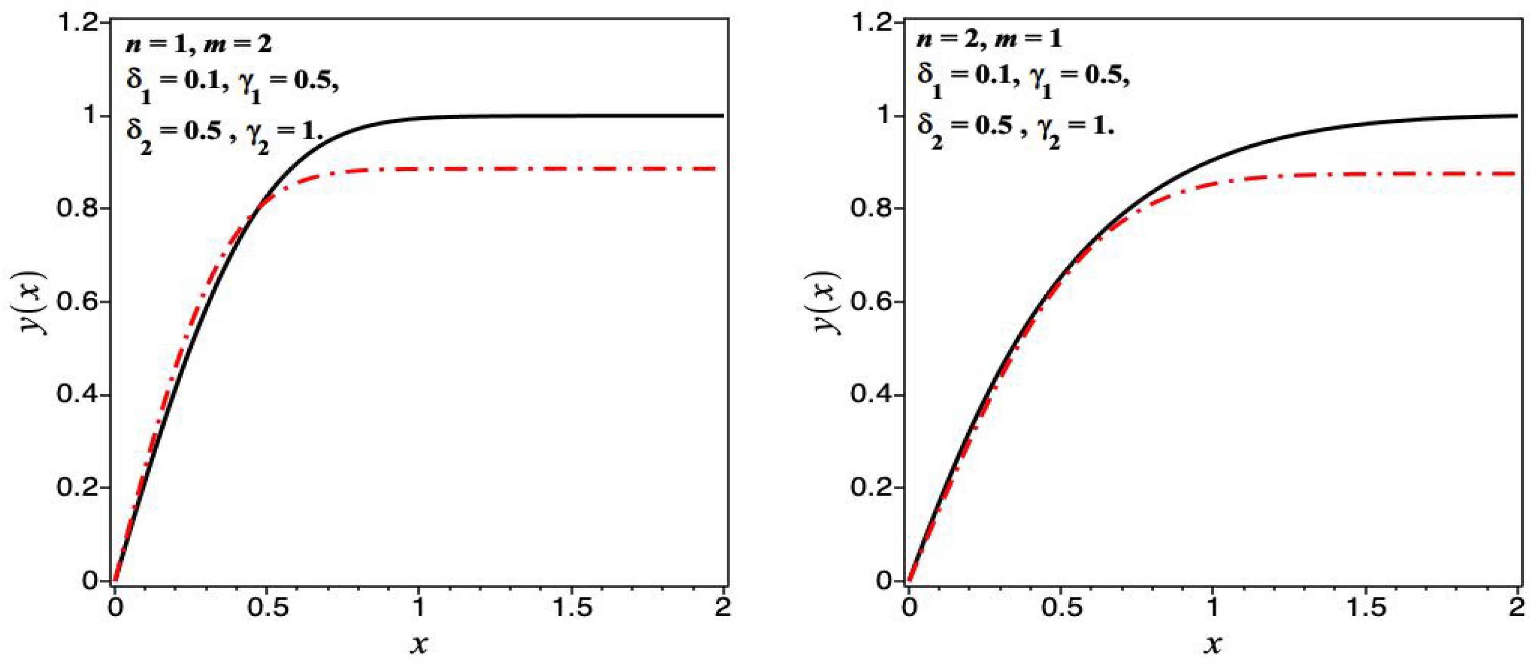
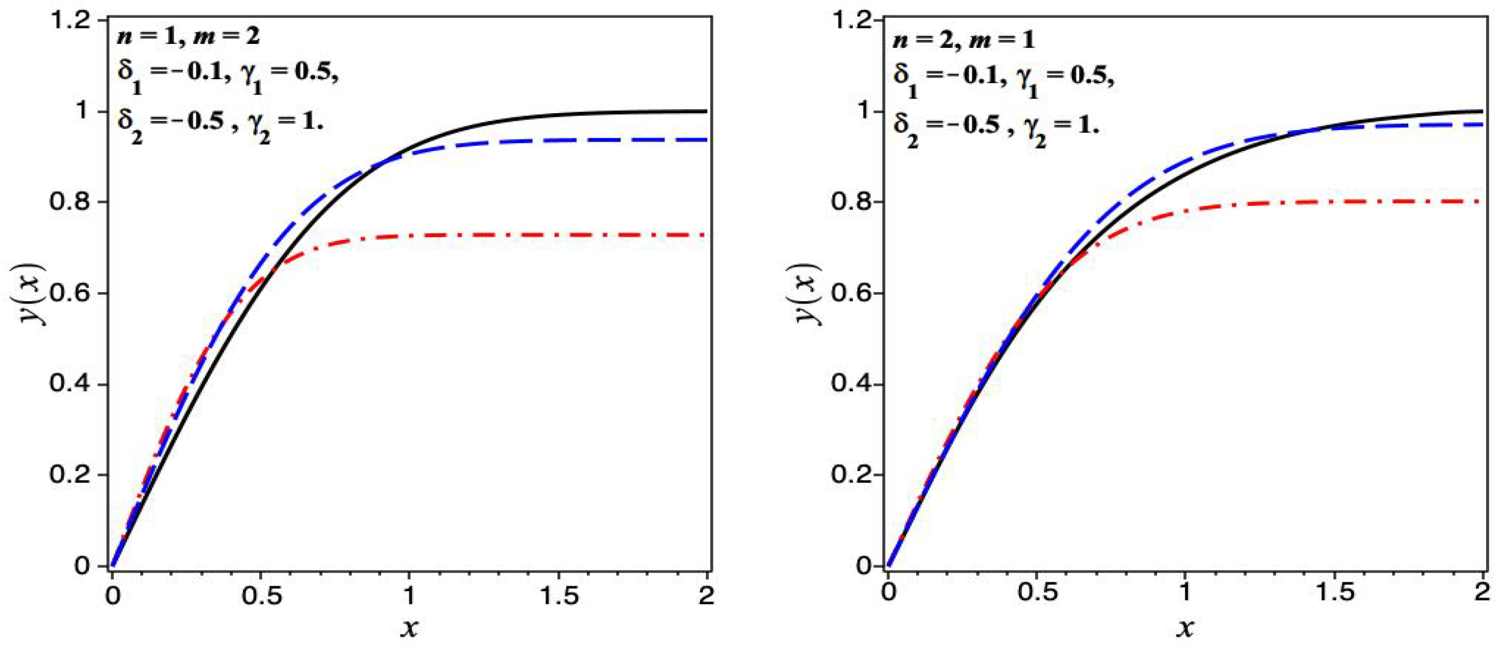
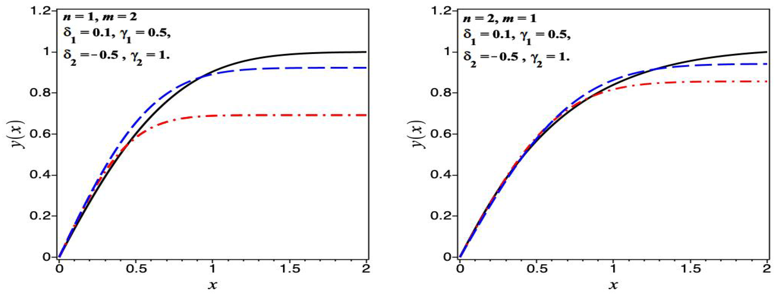
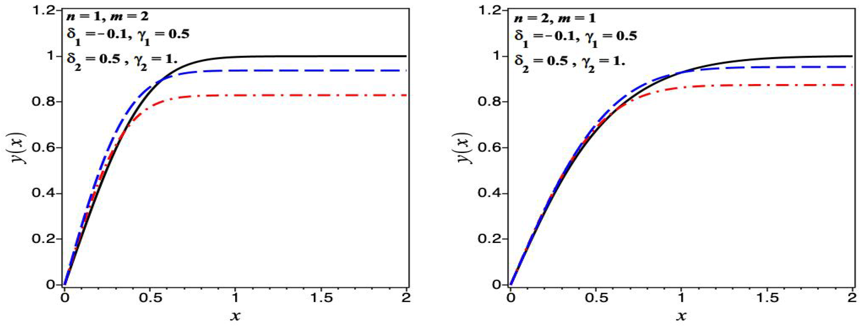
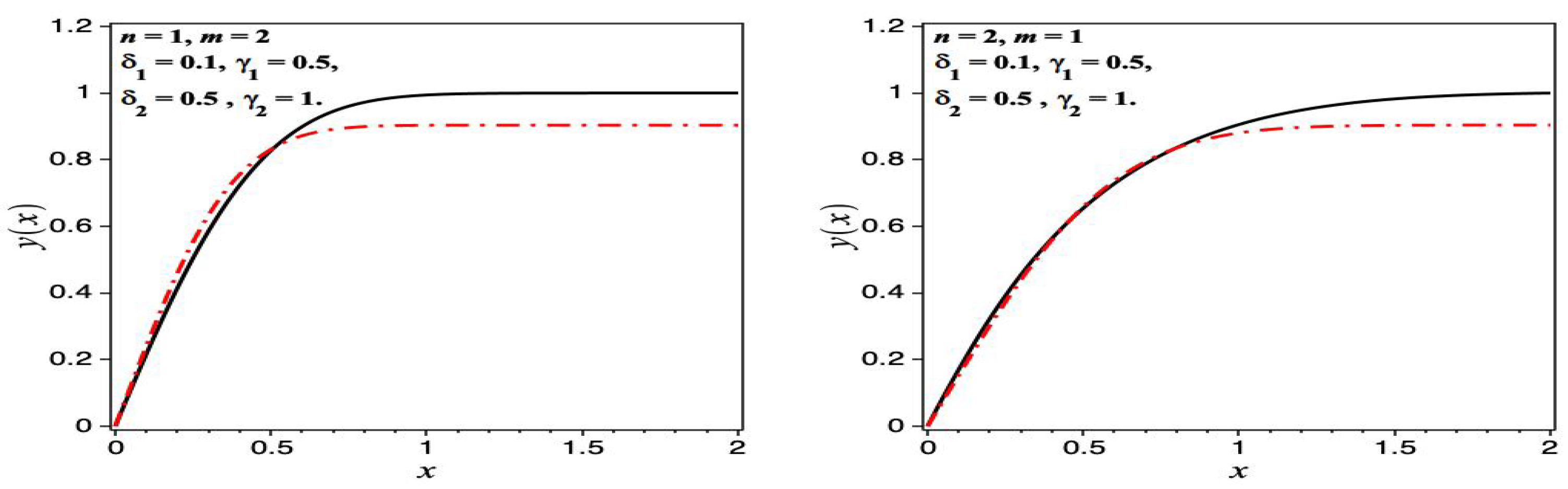
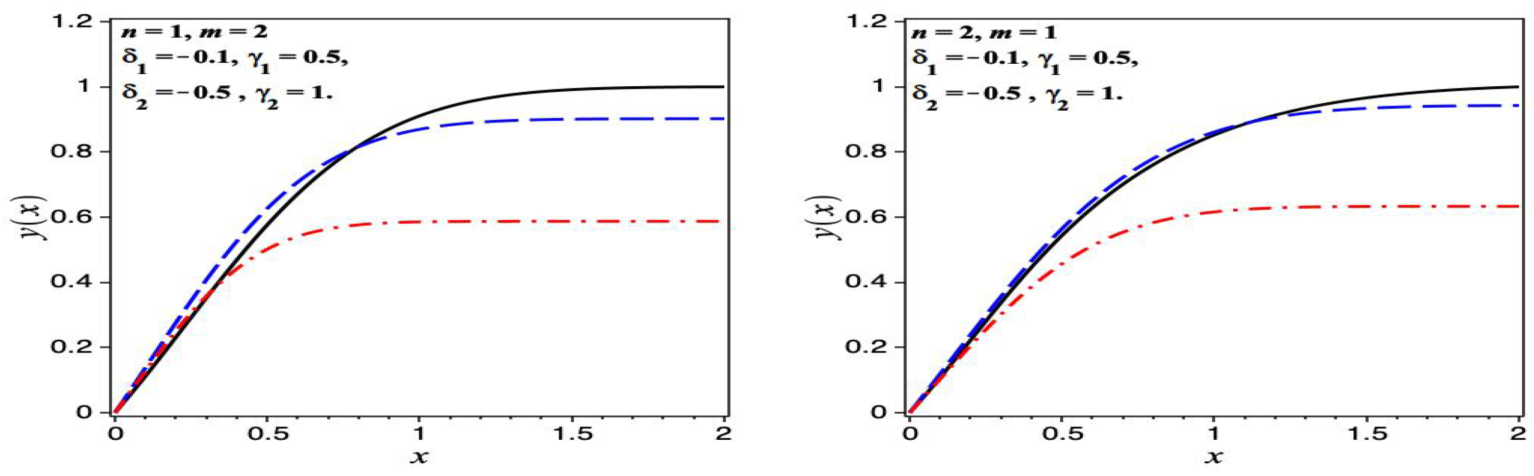
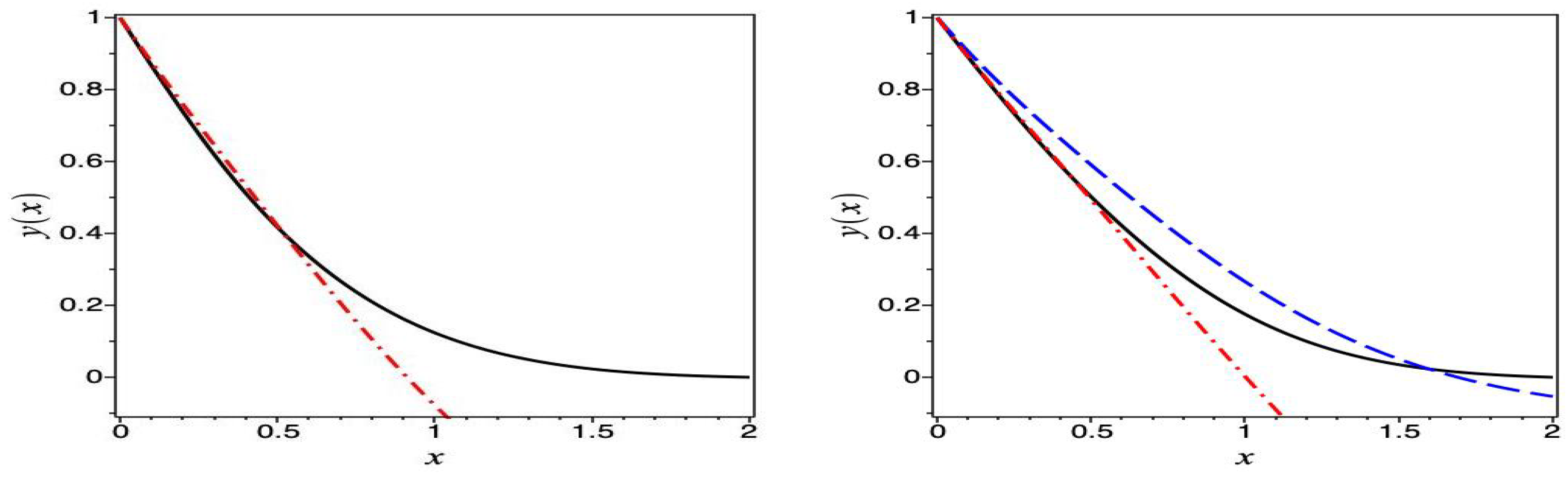
6. Numerical Results

6.1. Homogeneous Case

We used the capabilities of the robust Maple software for the rigorous numerical validation and developed an intuitively navigable program, featuring straightforward statements tailored to address boundary value problems (BVPs.).

Our program, based on the Maple software, possesses the capability to identify the nature of the problem at hand and autonomously select the most appropriate algorithm for its resolution.

In particular, we implemented the mid-defer method, an advanced midpoint technique that incorporates enhancement schemes. Among these enhancement schemes, the Richardson extrapolation method emerged as the fastest choice [41,42,43], while deferred corrections excelled in handling complex problems due to their lower memory usage. Furthermore, this method exhibited proficiency in addressing end-point singularities, a challenge that the trapezoidal scheme often struggles with.

The utilization of the continuation method is of paramount importance in minimizing global error while determining the optimal number of maximum mesh points. This numerical technique has been rigorously tested and proven effective in previous studies [44,45].

In Figure 1, we depict a comparative analysis involving the numerical solution and the lower solution for the first scenario and different values of ($n=1,m=2$) and ($n=2,m=1$), where ${\delta }_i\ge 0$, plotted against the independent variable x. This evaluation was conducted for a specific set of parameters: ${\delta }_1=0.1;{\delta }_2=0.5;{\gamma }_1=0.5;{\gamma }_2=1$, and the constant C was specifically assigned a value of $C=4$ for both cases.

Figure 1. The numerical solution and the lower bound of Pr. (4)–(5) for a specific parameter set, namely, ${\delta }_1=0.1;{\delta }_2=0.5;{\gamma }_1=0.5;{\gamma }_2=1$, and with the constant C set to $C=4$. Left panel $n=1,m=2$. Right panel $n=2,m=1$. The solid line corresponds to the numerical solution and the dash-dotted line corresponds to the lower bound.

The lower bound, which was chosen to conform to the condition $C_1\le C\le C_2$ in this particular case, exhibited a remarkable alignment with the numerical solution.

Figure 2 illustrates a comparative analysis involving the numerical solution and the lower solution $y_3\left(x\right)$ for two distinct scenarios: one with ($n=1,m=2$) and another with ($n=2,m=1$), all under the constraint that $-1<{\delta }_i<0$. The plotted data are presented against the independent variable x.

Figure 2. The numerical solution and the lower bound of Pr. (4)–(5) for a specific parameter set, namely, ${\delta }_1=-0.1;{\delta }_2=-0.5;{\gamma }_1=0.5;{\gamma }_2=1$. Left panel $n=1,m=2$, and $C=2.6$. Right panel $n=2,m=1$, and $C=3.2$. The solid line corresponds to the numerical solution and the dash-dotted line corresponds to the lower bound. The dashed blue line represents the lower bound $y_1\left(x\right)$ with $C\approx 2.222$, which can be chosen from $y_1(\infty )\simeq 1$.

This investigation utilized a specific parameter set: ${\delta }_1=-0.1,{\delta }_2=-0.5,{\gamma }_1=0.5$, ${\gamma }_2=1$. In both cases, a constant value of C was employed, with C taking the values 2.6 and 3.2, respectively. It is noteworthy to highlight that the lower bound $y_3\left(x\right)$ was in good accordance with the numerical solution for small values of the independent variable, i.e., $x\le 1$ when the constant C was thoughtfully chosen to adhere to the condition $C_3\le C\le C_4$ within this context. However, for larger values of $x\ge 1$, the numerical results indicate a rapid convergence of the solution in the first case.

We additionally present a plot of the lower bound, denoted by

$$y_1\left(x\right)=\frac{C\sqrt{\pi }}{2{({\gamma }_1+{\delta }_1+1)}^n\sqrt{{({\gamma }_2+{\delta }_2+1)}^m}}erf\left(\sqrt{{({\gamma }_2+{\delta }_2+1)}^m}x\right),$$

(indicated by the dashed blue line), which was carefully selected with an appropriate constant value, C, ensuring that $y_1(\infty )\simeq 1$. The selected lower bound, i.e., $y_1\left(x\right)$ to satisfy the condition $y_1(\infty )\simeq 1$ in this context, displayed a striking agreement with the numerical solution in the second case and can be considered as a good approximation.

Figure 3 presents a comparative examination involving the numerical solution and lower solution $y_5\left(x\right)$ for two distinctive scenarios: one characterized by ($n=1,m=2$) and the other by ($n=2,m=1$). These scenarios were subject to specific constraints: $-1<{\delta }_2<0$ and ${\delta }_1>0$. The plotted data are displayed as a function of the independent variable x.

Figure 3. The numerical solution and the lower bound of Pr. (4)–(5) for a specific parameter set, namely, ${\delta }_1=0.1;{\delta }_2=-0.5;{\gamma }_1=0.5;{\gamma }_2=1$. Left panel $n=1,m=2$, and $C=2.5$. Right panel $n=2,m=1$, and $C=3.5$. The solid line corresponds to the numerical solution and the dash-dotted line corresponds to the lower bound. The dashed blue line represents the lower bound $y_1\left(x\right)$, which can be chosen from $y_1(\infty )\simeq 1$.

We employed a parameter configuration for this analysis: ${\delta }_1=0.1;{\delta }_2=-0.5;{\gamma }_1=0.5;$${\gamma }_2=1$. Notably, both cases were governed by constant values of $C=2.5$ and $C=3.5$, respectively.

It is worth emphasizing that the lower boundary, carefully chosen to adhere to the condition $C_5\le C\le C_6$ in this context, exhibited a remarkable alignment with the numerical solution for small values of the independent variable $x\lesssim 1$.

We include a graph showing the lower bound, denoted by $y_1\left(x\right)$ (represented by the dashed blue line). This approximate solution was carefully chosen with a constant value, C, to ensure that $y_1(\infty )\simeq 1$. It is worth noting that the chosen approximate solution, i.e., $y_1\left(x\right)$, satisfies the condition $y_1(\infty )\simeq 1$ in this context, and it showed an excellent agreement with the numerical solution in the third case.

Figure 4 shows a comparative analysis involving the numerical solution and lower solution $y_7\left(x\right)$ for two distinct scenarios: one characterized by ($n=1,m=2$) and the other by ($n=2,m=1$). These scenarios were subject to specific constraints: ${\delta }_2>0$ and $-1<{\delta }_1<0$. The data plotted are represented as a function of the independent variable x.

Figure 4. The numerical solution and the lower bound of Pr. (4)–(5) for a specific parameter set, namely, ${\delta }_1=-0.1;{\delta }_2=0.5;{\gamma }_1=0.5;{\gamma }_2=1$ and $C=3.7$. Left panel $n=1,m=2$ and $C=3.7$. Right panel $n=2,m=1$, and $C=3.9$. The solid line corresponds to the numerical solution and the dash-dotted line corresponds to the lower bound. The dashed blue line represents the lower bound $y_1\left(x\right)$, which can be chosen from $y_1(\infty )\simeq 1$.

In this analysis, we utilized a parameter setup characterized by ${\delta }_1=0.1;{\delta }_2=-0.5;$${\gamma }_1=0.5;$${\gamma }_2=1$. It is important to note that the first case had a constant of $C=3.7$, while the second case had $C=3.9$.

It is noteworthy that the lower bound, thoughtfully chosen to satisfy the condition $C_7\le C\le C_8$ in this context, exhibited a remarkable alignment with the numerical solution for small values of $x\lesssim 1$.

We, again, include a graph that clearly shows the lower bound, denoted by $y_1\left(x\right)$, which is represented by the dashed blue line. This approximate solution was meticulously chosen with a constant value, C, to ensure that $y_1(\infty )\simeq 1$. It is crucial to note that the selected approximate solution, i.e., $y_1\left(x\right)$, satisfied the condition $y_1(\infty )\simeq 1$ in this context, and it exhibited an outstanding agreement with the numerical solution in the fourth case.

Based on the previous results, an interesting observation can be made regarding the numerical and approximated solutions. For small values of the independent variable $x\lesssim 1$, the numerical solution and the approximated solution, obtained using the lower bound with a carefully chosen constant C, exhibited perfect agreement. However, for large values ($x\gg 1$), a slight deviation between the solutions was noticeable. Nevertheless, it is worth noting that the numerical solutions converged rapidly to unity. Furthermore, the first lower-bound solution $y_1\left(x\right)$ aligned well with the numerical solution when the constant C was suitably chosen such that $y_1(\infty )\simeq 1$. This approximated solution can be considered the best approximation and called the limit superior to the lower bounds.

6.2. Nonhomogeneous Case

Now, we consider the nonhomogeneous Pr. (4)–(5) in the fourth case with the source term $\beta \left(x\right)=e^{-k{x}^2}$, where $k>0$. We restricted our exploration to two cases, i.e., ${\delta }_i>0$ and $-1<{\delta }_i<0$.

Figure 5 shows a comparative analysis involving the numerical solution and lower solution $y_7\left(x\right)$ for two distinct scenarios: one characterized by ($n=1,m=2$) and the other by ($n=2,m=1$). These scenarios were subject to specific constraints: ${\delta }_2>0$ and ${\delta }_1>0$. The data plotted are represented as a function of the independent variable x.

Figure 5. The numerical solution and the lower bound of Pr. (4)–(5) and $\beta \left(x\right)=e^{-k{x}^2}$ for a specific parameter set, namely, ${\delta }_1=0.1;{\delta }_2=0.5;{\gamma }_1=0.5;{\gamma }_2=1$. Left panel $n=1,m=2$. Right panel $n=2,m=1$. The constants D and k were chosen to be $D=3.9$ and $k=6.25$ for both cases. The solid line corresponds to the numerical solution and the dash-dotted line corresponds to the lower bound $w_1\left(x\right)$.

In this analysis, we utilized a parameter setup characterized by ${\delta }_1=0.1;{\delta }_2=0.5;{\gamma }_1=0.5;{\gamma }_2=1$. It is important to note that both cases had a constant of $D=3.9$, and $k=6.5$ such that $k⩾sup(k_1,k_2)$, where $k_1=\frac{1}{{({\gamma }_1+{\delta }_1+1)}^n}$ and $k_2={({\gamma }_2+{\delta }_2+1)}^m$.

For $x\lesssim 1$, the numerical solution aligned remarkably well with the lower bound $w_1\left(x\right)$, where D was chosen to satisfy $D_1\le D\le D_2$.

Figure 6 displays a comparison between the numerical solution and the lower solution $w_3\left(x\right)$ for two different situations. One scenario is characterized by ($n=1,m=2$) while the other is characterized by ($n=2,m=1$). Both scenarios had specific constraints: $-1<{\delta }_2<0$ and $-1<{\delta }_1<0$. The data plotted are a function of the independent variable x.

Figure 6. The numerical solution and the lower bound for boundary problem (4) with boundary conditions (5) and $\beta \left(x\right)=e^{-k{x}^2}$ for a specific parameter set, namely, ${\delta }_1=0.1;{\delta }_2=0.5;{\gamma }_1=0.5;{\gamma }_2=1$. Left panel $n=1,m=2$ and $D=1.9$. Right panel $n=2,m=1$ and $D=3.9$. The constant k was chosen to be $k=6.25$ for both cases. The solid line corresponds to the numerical solution and the dash-dotted line corresponds to the lower bound $w_3\left(x\right)$. The dashed blue line represents the approximate solution $w_1\left(x\right)$ with the suitable choice of the constant D such that $w_1\left(x\right)\approx 1$. The dashed blue line represents the lower bound $w_1\left(x\right)$ with $w_1(\infty )\simeq 1$.

In our analysis, we used the following parameter setup: ${\delta }_1=-0.1$, ${\delta }_2=-0.5$, ${\gamma }_1=0.5$, and ${\gamma }_2=1$. It is worth noting that both cases had a constant of $D=1.9$ and $D=3.9$, respectively. The constant k was chosen to be $k=6.5$ such that $k⩾sup(k_3,k_4)$, where $k_3=\frac{{({\delta }_2+1)}^m}{{({\gamma }_1+1)}^n}$ and $k_2=\frac{{({\gamma }_2+1)}^m}{{({\delta }_1+1)}^n}$. When $x\lesssim 1$, the numerical solution was in good agreement with the lower bound $w_3\left(x\right)$. We chose D to satisfy $D_3\le D\le D_4$. To make things clearer, we include a graph that shows the lower bound, represented by the dashed blue line and denoted as

$$w_1\left(x\right)=\frac{D\sqrt{\pi }}{2{({\gamma }_1+{\delta }_1+1)}^n\sqrt{{({\gamma }_2+{\delta }_2+1)}^m}}erf\left(\sqrt{{({\gamma }_2+{\delta }_2+1)}^m}x\right)$$

$$+\frac{\sqrt{\pi }}{2{({\gamma }_1+{\delta }_1+1)}^n\sqrt{k-\frac{1}{{({\gamma }_1+{\delta }_1+1)}^n}}}{\int }_0^x{e}^{-{({\gamma }_2+{\delta }_2+1)}^m{\eta }^2}erf\left(\sqrt{k-\frac{1}{{({\gamma }_1+{\delta }_1+1)}^n}}\eta \right)d\eta ,$$

with $k>\frac{1}{{({\gamma }_1+{\delta }_1+1)}^n}$.

We carefully selected this approximate solution to ensure that $w_1(\infty )\simeq 1$, using a constant value of D. It is important to note that the chosen solution, $w_1\left(x\right)$, closely matched the numerical solution.

Finally, we explore the nonhomogeneous problem (4)–(6), in addition to the source term $\beta \left(x\right)=e^{-k{x}^2}$, where $k>0$. We limited our analysis to two cases, i.e., ${\delta }_i>0$ and $-1<{\delta }_i<0$.

Figure 7 displays a comparison between the numerical solution and the lower solution $v_1\left(x\right),v_3\left(x\right)$ for two different situations, respectively. The first scenario was characterized by ${\delta }_i>0$, while the second was characterized by $-1<{\delta }_i<0.$ Both scenarios had specific constants: $n=1,m=2$. The data plotted are a function of the independent variable x. The dashed blue line in the right panel represents the good approximation of the solution $v_1\left(x\right)$ such that $v_1\left(x\right)\approx 1$.

Figure 7. The numerical solution and the lower bound for boundary problem (4) with boundary conditions (6) and $\beta \left(x\right)=e^{-k{x}^2}$ for a specific parameter set, namely, ${\delta }_1=0.1;{\delta }_2=0.5;{\gamma }_1=0.5;{\gamma }_2=1$ (left panel) and ${\delta }_1=-0.1;{\delta }_2=-0.5;{\gamma }_1=0.5;{\gamma }_2=1$ (right panel). In both cases $n=1,m=2$. The constants E and k were chosen to be $E=-1.$ and $k=6.25$ for both cases. The solid line corresponds to the numerical solution and the dash-dotted line corresponds to the corresponding lower bound $v_1\left(x\right),v_3\left(x\right)$, respectively. The dashed blue line in the right panel represents the good approximation that is chosen as $v_1\left(x\right)$ such that $n_1\left(x\right)\approx 1$.

Throughout the previous instances, solely the lower bounds exhibited a notable approximation to the numerical solution. We omitted the upper bounds due to their lack of this advantageous alignment. This outcome aligned with our expectations as the upper bounds were characterized by functions displaying exponential growth.

However, justifying the selection of initial constants (C and D) in approximate solutions for homogeneous and nonhomogeneous equations to ensure their alignment with numerical solutions can be approached using various methods. Initially, confirming that the initial or boundary conditions specified in the approximate solutions correspond with those utilized in the numerical solutions is essential. Subsequently, adjusting the constants C and D is necessary to meet these conditions. Additionally, conducting an error analysis between the analytical solution (using initial constants C and D) and the numerical solution is crucial. The aim here is to minimize the error by adjusting the values of C and D, striving for the closest agreement between both solutions. Moreover, verifying that the assumptions and constraints utilized in deriving the approximate solutions are consistent with those inherent in the numerical method is vital. Adjusting C and D accordingly helps maintain coherence between the models. These aspects were all considered in our analysis and the selection of constants adhered to these principles.

7. Conclusions

The Stefan problem with nonlinear thermal conductivity and specific heat properties was thoroughly explored. This study employed lower- and upper-bound techniques to establish the existence and uniqueness of the theorem, addressing both homogeneous and nonhomogeneous scenarios. Additionally, a detailed numerical analysis was conducted, yielding a highly accurate approximation solution. Moreover, the alignment between the lower bound and the numerical solution, achieved through a suitable selection of the constant, confirms the validity of the chosen bounding techniques. This agreement not only validates the reliability of these techniques in delineating the system’s response but also offers valuable insights into the behavior of the solution to the problem. Additionally, it acts as a confirmation of the efficacy of the employed analytical methods. Such methodologies pave the path for the investigation of analogous challenges in forthcoming research endeavors. Understanding and interpreting solutions to the nonclassical Stefan problem holds paramount significance in material design, thermal management, and process optimization—making it an essential aspect across the scientific, engineering, and technological domains.

References

- Cho, S.H.; Sunderland, J.E. Phase Change Problems With Temperature-Dependent Thermal Conductivity. J. Heat Transf. 1974, 96, 214–217. [Google Scholar] [CrossRef]
- Oliver, D.; Sunderland, J. A phase change problem with temperature-dependent thermal conductivity and specific heat. Int. J. Heat Mass Transf. 1987, 30, 2657–2661. [Google Scholar] [CrossRef]
- Ceretani, A.N.; Salva, N.N.; Tarzia, D.A. Existence and uniqueness of the modified error function. Appl. Math. Lett. 2017, 70, 14–17. [Google Scholar] [CrossRef]
- Bougouffa, S.; Khanfer, A.; Bougoffa, L. On the approximation of the modified error function. Math. Methods Appl. Sci. 2022, 46, 11657–11665. [Google Scholar] [CrossRef]
- Khanfer, A.; Bougoffa, L. A Stefan problem with nonlinear thermal conductivity. Math. Methods Appl. Sci. 2022, 46, 4602–4611. [Google Scholar] [CrossRef]
- Briozzo, A.C.; Tarzia, D.A. Existence, Uniqueness and an Explicit Solution for a One-Phase Stefan Problem for a Non-classical Heat Equation, Free Boundary Problems. Int. Ser. Numer. Math. 2006, 154, 117–124. [Google Scholar]
- Bougoffa, L. A note on the existence and uniqueness solutions of the modified error function. Math. Methods Appl. Sci. 2018, 41, 5526–5534. [Google Scholar] [CrossRef]
- Bougoffa, L.; Rach, R.; Mennouni, A. On the existence, uniqueness, and new analytic approximate solution of the modified error function in two-phase Stefan problems. Math. Methods Appl. Sci. 2021, 44, 10948–10956. [Google Scholar] [CrossRef]
- Zhou, Y.; Xia, L.-J. Exact solution for Stefan problem with general power-type latent heat using Kummer function. Int. J. Heat Mass Transf. 2015, 84, 114–118. [Google Scholar] [CrossRef]
- Kumar, A.; Singh, A.K.; Rajeev. A moving boundary problem with variable specific heat and thermal conductivity. J. King Saud Univ.-Sci. 2020, 32, 384–389. [Google Scholar] [CrossRef]
- Chen, X.; Lou, B.; Zhou, M.; Giletti, T. Long time behavior of solutions of a reaction-diffusion equation on unbounded intervals with Robin boundary conditions. Ann. Inst. H. Poincare Anal. non lin. 2016, 33, 67–92. [Google Scholar] [CrossRef]
- Ribera, H.; Myers, T.G. A mathematical model for nanoparticle melting with size-dependent latent heat and melt temperature. Microfluid. Nanofluidics 2016, 20, 147. [Google Scholar] [CrossRef]
- Font, F.; Myers, T.G.; Mitchell, S.L. A mathematical model for nanoparticle melting with density change. Microfluid. Nanofluid. 2015, 18, 233–243. [Google Scholar] [CrossRef]
- Briozzo, A.C.; Natale, M.F. One-phase Stefan problem with temperature-dependent thermal conductivity and a boundary condition of Robin type. J. Appl. Anal. 2015, 21, 89–97. [Google Scholar] [CrossRef]
- Bougoffa, L.; Khanfer, A. On the solutions of a phase change problem with temperature-dependent thermal conductivity and specific heat. Results Phys. 2020, 19, 103646. [Google Scholar] [CrossRef]
- Voller, V.; Swenson, J.; Paola, C. An analytical solution for a Stefan problem with variable latent heat. Int. J. Heat Mass Transf. 2004, 47, 5387–5390. [Google Scholar] [CrossRef]
- Beasley, J.D. Thermal conductivities of some novel nonlinear optical materials. Appl. Opt. 1994, 33, 1000–1003. [Google Scholar] [CrossRef]
- Aggarwal, R.L.; Fan, T.Y. Thermal diffusivity, specific heat, thermal conductivity, coefficient of thermal expansion, and refractive-index change with temperature in AgGaSe2. Appl. Opt. 2005, 44, 2673–2677. [Google Scholar] [CrossRef]
- Henager, C.H.; Pawlewicz, W.T. Thermal conductivities of thin, sputtered optical films. Appl. Opt. 1993, 32, 91. [Google Scholar] [CrossRef]
- de Azevedo, A.M.; dos Santos Magalhães, E.; da Silva, R.G.D. A comparison between nonlinear and constant thermal properties approaches to estimate the temperature in LASER welding simulation. Case Stud. Therm. Eng. 2022, 35, 102135. [Google Scholar] [CrossRef]
- Xiao, Y.; Wu, H. An explicit coupled method of FEM and meshless particle method for simulating transient heat transfer process of friction stir welding. Math. Probl Eng. 2020, 2020, 2574127. [Google Scholar] [CrossRef]
- Brizes, E.; Jaskowiak, J.; Abke, T.; Ghassemi-Armaki, H.; Ramirez, A.J. Evaluation of heat transfer within numerical models of resistance spot welding using high-speed thermography. J. Mater. Process. Technol. 1985, 297, 117276. [Google Scholar] [CrossRef]
- Gladkov, S.O.; Bogdanova, S.B. On the theory of nonlinear thermal conductivity. Tech. Phys. 2016, 61, 157–164. [Google Scholar] [CrossRef]
- Sahoo, R.; Sarangi, S. Effect of temperature-dependent specific heat of the working fluid on the performance of cryogenic regenerators. Cryogenics 1985, 25, 583–590. [Google Scholar] [CrossRef]
- Tomeczek, J.; Palugniok, H. Specific heat capacity and enthalpy of coal pyrolysis at elevated temperatures. Fuel 1996, 75, 1089–1093. [Google Scholar] [CrossRef]
- Saxena, S.K. Earth mineralogical model: Gibbs free energy minimization computation in the system MgO-FeO-SiO2. Geochim. Cosmochim. Acta 1996, 60, 2379–2395. [Google Scholar] [CrossRef]
- Merrick, D. Mathematical models of the thermal decomposition of coal: 2. Specific heats and heats of reaction. Fuel 1983, 62, 540–546. [Google Scholar] [CrossRef]
- Hanrot, F.; Ablitzer, D.; Houzelot, J.; Dirand, M. Experimental measurement of the true specific heat capacity of coal and semicoke during carbonization. Fuel 1994, 73, 305–309. [Google Scholar] [CrossRef]
- Haemmerich, D.; dos Santos, I.; Schutt, D.J.; Webster, J.G.; Mahvi, D.M. In vitro measurements of temperature-dependent specific heat of liver tissue. Med. Eng. Phys. 2006, 28, 194–197. [Google Scholar] [CrossRef]
- Ghosh, A.; McSween, H.Y. Temperature dependence of specific heat capacity and its effect on asteroid thermal models. Mefeorifrcs Planet. Sci. 1999, 34, 121–127. [Google Scholar] [CrossRef]
- Scott, E.P. An Analytical Solution and Sensitivity Study of Sublimation-Dehydration Within a Porous Medium With Volumetric Heating. J. Heat Transf. 1994, 116, 686–693. [Google Scholar] [CrossRef]
- Menaldi, J.L.; Tarzia, D.A. Generalized Lamé–Clapeyron solution for a one-phase source Stefan problem. Comput. Appl. Math. 1993, 12, 123–142. [Google Scholar]
- Briozzo, A.C.; Natale, M.F.; Tarzia, D.A. Explicit solutions for a two-phase unidimensional Lamé–Clapeyron–Stefan problem with source terms in both phases. J. Math. Anal. Appl. 2007, 329, 145–162. [Google Scholar] [CrossRef]
- Briozzo, A.C.; Tarzia, D.A. A Stefan problem for a non-classical heat equation with a convective condition. Appl. Math. Comput. 2010, 217, 4051–4060. [Google Scholar] [CrossRef]
- Briozzo, A.C.; Tarzia, D.A. Exact Solutions for Nonclassical Stefan Problems. Int. J. Differ. Equ. 2010, 2010, 868059. [Google Scholar] [CrossRef]
- Briozzo, A.C.; Natale, M.F. Two Stefan problems for a non-classical heat equation with nonlinear thermal coefficients. Differ. Integral Equ. 2014, 27, 1187–1202. [Google Scholar] [CrossRef]
- Briozzo, A.C.; Natale, M.F. Non-classical Stefan problem with nonlinear thermal coefficients and a Robin boundary condition. Nonlinear Anal. Real World Appl. 2019, 49, 159–168. [Google Scholar] [CrossRef]
- Bollati, J.; Natale, M.F.; Semitiel, J.A.; Tarzia, D.A. Exact solution for non-classical one-phase Stefan problem with variable thermal coefficients and two different heat source terms. Comput. Appl. Math. 2022, 41, 375. [Google Scholar] [CrossRef]
- Bougoffa, L.; Bougouffa, S.; Khanfer, A. An Analysis of the One-Phase Stefan Problem with Variable Thermal Coefficients of Order p. Axioms 2023, 12, 497. [Google Scholar] [CrossRef]
- Willett, D. Uniqueness for second order nonlinear boundary value problems with applications to almost periodic solutions. Ann. Mat. Pura Appl. 1969, 81, 77–92. [Google Scholar] [CrossRef]
- Quarteroni, A.; Sacco, R.; Saleri, F. Numerical Mathematics; Springer Science & Business Media: Berlin/Heidelberg, Germany, 2007. [Google Scholar]
- Hamming, R. Numerical Methods for Scientists and Engineers; Courier Corporation: Chelmsford, MA, USA, 1987. [Google Scholar]
- Ascher, U.; Petzold, L. Computer Methods for Ordinary Differential Equations and Differential-Algebraic Equations; SIAM: Philadelphia, PA, USA, 1998. [Google Scholar]
- Bougoffa, L.; Bougouffa, S.; Khanfer, A. Generalized Thomas-Fermi equation: Existence, uniqueness, and analytic approximation solutions. AIMS Math. 2023, 8, 10529–10546. [Google Scholar] [CrossRef]
- Khanfer, A.; Bougoffa, L.; Bougouffa, S. Analytic Approximate Solution of the Extended Blasius Equation with Temperature-Dependent Viscosity. J. Nonlinear Math. Phys. 2023, 30, 287–302. [Google Scholar] [CrossRef]
Disclaimer/Publisher’s Note: The statements, opinions and data contained in all publications are solely those of the individual author(s) and contributor(s) and not of MDPI and/or the editor(s). MDPI and/or the editor(s) disclaim responsibility for any injury to people or property resulting from any ideas, methods, instructions or products referred to in the content. |
© 2023 by the authors. Licensee MDPI, Basel, Switzerland. This article is an open access article distributed under the terms and conditions of the Creative Commons Attribution (CC BY) license (https://creativecommons.org/licenses/by/4.0/).