Article

Estimation of Entropy for Generalized Rayleigh Distribution under Progressively Type-II Censored Samples

1
Teaching Department of Basic Subjects, Jiangxi University of Science and Technology, Nanchang 330013, China
2
College of Science, Jiangxi University of Science and Technology, Ganzhou 341000, China
*
Author to whom correspondence should be addressed.
Axioms 2023, 12(8), 776; https://doi.org/10.3390/axioms12080776
Submission received: 11 July 2023 / Revised: 6 August 2023 / Accepted: 9 August 2023 / Published: 10 August 2023
(This article belongs to the Special Issue Statistical Methods and Applications)

Abstract

:
This paper investigates the problem of entropy estimation for the generalized Rayleigh distribution under progressively type-II censored samples. Based on progressively type-II censored samples, we first discuss the maximum likelihood estimation and interval estimation of Shannon entropy for the generalized Rayleigh distribution. Then, we explore the Bayesian estimation problem of entropy under three types of loss functions: K-loss function, weighted squared error loss function, and precautionary loss function. Due to the complexity of Bayesian estimation computation, we use the Lindley approximation and MCMC method for calculating Bayesian estimates. Finally, using a Monte Carlo statistical simulation, we compare the mean square errors to examine the superiority of maximum likelihood estimation and Bayesian estimation under different loss functions. An actual example is provided to verify the feasibility and practicality of various estimations.

1. Introduction

The Rayleigh distribution has many practical applications in reliability and life testing, and typically used in physical modeling processes in different fields such as wave heights in the ocean, sound and light radiation, wireless signals and wind energy, and ultrasound imaging modeling [1]. It is also used for modeling resistors, networks, crystals, relays, and capacitors in aircraft radar assemblies with lifetimes of only a few hours. In all of these applications, it is generally assumed that the lifetime of a particular device depends on its age. Because generalized models based on lifetime distributions have more intuitive applicability and attractiveness in the modeling process, Surles and Padgett [2] proposed the two-parameter Burr Type X distribution, also known as the generalized Rayleigh distribution. They studied the statistical characteristics and some properties of the generalized Rayleigh distribution, and pointed out that it can be used as a lifetime distribution and to characterize intensity data. Surles et al. [3] and Al-khedhari et al. [4] discussed parameter estimation for this distribution using different techniques.
The generalized Rayleigh distribution is essentially a two-parameter Burr Type X distribution [1], which was first introduced by Surles and Padgett in 2001 [2]. Burr Type X and Burr Type XII distributions are important distributions in survival analysis problems. They were two of the twelve types of lifetime distributions proposed by Burr in 1942, and since their proposal, their applications and statistical inference theory have received widespread attention and research [3,4]. In recent years, with the deepening of research, the generalized Rayleigh distribution has been widely applied in fields such as wireless communication, radar signal processing, image processing, seismology, astronomy, and ecology [5,6,7]. It not only meets the needs for different types of data, such as the distribution of radio signal strength, power load, and seismic wave energy, but also provides more accurate data analysis methods and tools to help us better understand and interpret data in various practical problems. In addition, the generalized Rayleigh distribution is an extension of the Rayleigh distribution. Compared with the Rayleigh distribution, the generalized Rayleigh distribution has more superior performance. It can better fit the data in some practical problems by introducing additional parameters and variables. The Rayleigh distribution is usually used to describe amplitude distribution, but in some cases, different types of data distribution such as amplitude, power, and energy may require more complex models. Therefore, the generalized Rayleigh distribution has played a role in improving existing models and providing more accurate and comprehensive descriptions and analysis [8]. Based on ranked set sampling (RSS), Shen et al. [9] compared the performance of RSS with respect to simple random sampling by observing modified unbiased and modified best linear unbiased estimators from generalized Rayleigh distribution. They found that the prementioned estimators based on RSS were significantly more efficient than the ones in SRS. Shen et al. [10] applied the generalized Rayleigh distribution to real-life scenarios, using its heavy-tailed property for Reddit ads and breast cancer datasets, and compared it with other generalized Rayleigh distributions. Rabie et al. [11] studied the lifetime analysis of devices following the generalized Rayleigh distribution under a type-II mixed censored scheme, obtaining Bayes estimates and E-Bayes estimates using a squared error loss function and linear loss function. It can be seen that the generalized Rayleigh distribution not only helps to expand the scope of application of the Rayleigh distribution and improve the accuracy and reliability of data analysis, but also provides theoretical support for the modeling and prediction of practical problems. Therefore, it is meaningful to study the generalized Rayleigh distribution in this paper.
Let X be a random variable that follows a generalized Rayleigh distribution with parameters β and σ , denoted by G R D ( σ , β ) . The probability density function (PDF) and cumulative distribution function are, respectively, as follows:
f ( x | σ , β ) = 2 σ β 2 x e β 2 x 2 ( 1 e β 2 x 2 ) σ 1 ,   x > 0 ,   σ ,   β > 0 ,
F ( x | σ , β ) = ( 1 e β 2 x 2 ) σ ,   x > 0 ,   σ ,   β > 0 .
Here, σ and β are the shape and scale parameters of the G R D ( σ , β ) .
The survival function and hazard function (HF) of G R D ( σ , β ) are, respectively, as follows:
r ( x | σ , β ) = 1 ( 1 e β 2 x 2 ) σ ,   x > 0 ,   σ ,   β > 0 ,
h ( x | σ , β ) = 2 σ β 2 x e β 2 x 2 ( 1 e β 2 x 2 ) σ 1 1 ( 1 e β 2 x 2 ) σ ,   x > 0 ,   σ ,   β > 0 .
The PDF and HF of the G R D ( σ , β ) are closely related to the parameters σ and β . Raqab and Kundu [12] pointed out that when σ = 1 , the distribution is a standard Rayleigh distribution. When σ 1 , σ serves as the shape parameter of the distribution. When σ > 1 / 2 , the PDF is a decreasing function, and the graph of HF exhibits a bathtub shape. When σ 1 / 2 , the PDF is a right-skewed unimodal function, and the graph of HF shows an increasing shape. The image of the PDF and HF of the G R D ( σ , β ) is shown in Figure 1.
This paper considers the estimation problem of the G R D ( σ , β ) . In Section 2, the Shannon entropy of G R D ( σ , β ) is firstly derived and the maximum likelihood(ML) estimation and asymptotic confidence interval (ACI) estimation of Shannon entropy are discussed. Section 3 performs the Bayes estimators (BEs) under the weighted squared error loss function (WESLF), precautionary loss function (PLF) and K-loss function (KLF), and numerically calculates these estimators using Lindley’s approximation and the MCMC method. Section 4 observes the performance of each estimation method using a Monte Carlo simulation. In Section 5, the superiority of the estimation methods used is compared using real data. Finally, conclusions are given in Section 6.

2. Preliminary Knowledge

2.1. Shannon Entropy of G R D ( σ , β )

Shannon entropy is an important concept in information theory used to measure the uncertainty or randomness of information. It was introduced by Shannon in 1948 and is considered one of the foundations of information theory. Shannon entropy is defined as follows:
H ( f ) = 0 f ( x ) ln f ( x ) d x
where f ( x ) is the PDF of a continuous random variable X .
In the existing literature, there have been significant advancements in the estimation of entropy functions for different distributions. Xu and Gui [13] discussed the estimation problem of entropy for the two-parameter inverse Weibull distribution under an adaptive Type-II progressive hybrid censoring scheme. Chacko and Asha [14] discussed the entropy estimation problem for the generalized exponential distribution based on record values. Shrahili et al. [15] discussed the estimation of logarithmic logistic distribution entropy under asymptotic testing. Wang and Gui [16] used the ML estimation and Bayesian estimation methods to obtain an estimate of the entropy of the two-parameter Burr type distribution under progressively censoring data. Al-Babtain et al. [17] analyzed the estimation of entropy for the Kumaraswamy distribution using ML estimation. Bantan et al. [18] discussed the estimation of entropy for the inverse Lomax distribution under multiple censoring data. Shi et al. [19] discussed the estimation of entropy for the generalized Bilal distribution under adaptive Type-II hybrid censored data and obtained ML estimates of entropy and parameters using Newton’s iteration method. Liu and Gui [20] discussed the estimation problem of entropy for the two-parameter Lomax distribution under generalized asymptotic hybrid censored data. They estimated entropy by deriving the ML estimation of unknown parameters and analyzed BEs under different loss functions, obtaining Bayesian estimates using the Lindley approximation method and MCMC method.
Theorem 1.
Let X be a random variable whose PDF is  G R D ( σ , β )  in Equation (1). Then, the Shannon entropy of the  G R D ( σ , β )  is
H ( f ) = ln 2 σ β 2 σ i = 0 ( σ 1 i ) ( 1 ) i 1 2 Γ ( 1 ) Γ ( 1 ) ln [ β ( 1 + i ) 1 2 ] 1 + i + [ φ ( σ + 1 ) φ ( 1 ) ] 1 σ + 1 .
here,  φ ( . )  represents the digamma function, and  Γ ( . )  represents the gamma function.
Proof. 
See Appendix A. □

2.2. Maximum Likelihood Estimation

At present, most of the research on the Rayleigh distribution is based on the analysis of sample data under complete or censored data. However, because there are some irresistible factors in the process of the test, such as time factors, test funds, etc., we chose to use the censored test method for the life test. The commonly used censored life tests include timed (Type-I) censored tests and fixed number (Type-II) censored tests [21]. Due to the fact that the timed and fixed number censored tests terminate the test after reaching the censored time and a certain sample size, and do not remove any products, it is easy to cause certain errors in the conclusions obtained from the test in both cases [3]. Therefore, the gradually censoring test is applicable. Generally, there are progressive Type-I censored (PC-I) tests and progressive Type-II censored (PC-II) tests, both of which are censored test methods that can be terminated in advance, thereby saving test costs and time [22]. This paper discusses the estimation of the entropy of the G R D ( σ , β ) under the Type-II censoring test. The advantage of the stepwise Type-II consored test is that it can remove some of the products that have not failed during different specified testing stages to analyze the performance of the products. Using this test method can flexibly adjust the sample size and consored time, more effectively utilize time and resources, and thus improve the efficiency of data collection. From a practical perspective, compared to the traditional Type-II censored scheme, this censored scheme can determine the sample size based on the actual needs and currently available resources. By gradually increasing the sample size, resources are maximized while ensuring product quality, avoiding resource waste while ensuring the accuracy of the obtained data. At the same time, the censored plan can also set the censored time according to the actual situation. By gradually increasing the censored time, it can save time to the maximum extent while ensuring product quality, thereby avoiding time consumption and improving the reliability of data analysis.
Assuming a life test is conducted on n products, each time a failed product is observed, a certain number of products are randomly removed from the remaining non-failed products [23]. That is to say, when the failure time of the first product is observed to be X 1 : m : n , P 1 products are removed from the remaining n 1 non-failed products, and n 1 P 1 products remain to be observed. When the expiration time of the second product is observed to be X 2 : m : n , P 2 products are removed from the remaining non-expired products, leaving n 2 P 1 P 2 products; continuing this way, when the failure time of the m-th product is observed to be X m : m : n , the experiment is stopped and P m products are removed, P m = n m P 1 P 2 P m 1 .
Let ( X 1 : m : n , X 2 : m : n , , X m : m : n ) be the m PC-II samples observed from n total test samples, and each X i : m : n   ( 0   <   i     m ) follows the G R D ( σ , β ) defined by Equation (1). According to the literature [24], based on the PC-II sample, the likelihood function (LF) can be defined as follows:
L ( σ , β | x ) = q i = 1 m f ( x i : m : n ) [ 1 F ( x i : m : n ) ] P i ,
where q = n ( n P 1 1 ) ( n P 1 P 2 ) ( n i = 1 m 1 ( P i + 1 ) ) , and x i : m : n represents the observation values of the X i : m : n sample. For convenience, we briefly write x i : m : n as x i , and x = ( x 1 , x 2 , , x m ) . Substituting Equations (1) and (2) into Equation (5), we can obtain
L ( σ , β | x ) = 2 m σ m β 2 m q i = 1 m ( x i ( 1 u i ) u i σ 1 ( 1 u i σ ) P i ) ,
where u ( β , x ) = 1 e β 2 x 2 .
The corresponding log-LF is
l ( σ , β ) = ln L ( σ , β | x ) = m ln 2 + m ln σ + 2 m ln β + ln q + i = 1 m ln x i + i = 1 m ln ( 1 u i )   + ( σ 1 ) i = 1 m ln u i + i = 1 m P i ln ( 1 u i σ ) .
The likelihood equations are as follows:
l ( σ , β ) σ = m σ + i = 1 m ln u i i = 1 m P i u i σ ln u i 1 u i σ = 0 ,
l ( σ , β ) β = 2 m β 2 β i = 1 m x i 2 + 2 β i = 1 m [ x i 2 ( 1 u i ) ( σ 1 ) u i σ P i x i 2 ( 1 u i ) u i σ 1 1 u i σ ] = 0 .
By solving Equations (8) and (9), σ and β can be obtained. It should be noted that the ML estimators of these equations cannot be analytically determined, so we need to use numerical calculation methods to calculate σ and β . Now, we introduce the following algorithm to solve the ML estimators of σ and β , the steps of which are given as follows:
(i)
Determine the LF and take the logarithm to obtain the log-LF.
(ii)
Calculate the first derivative and the second derivative of the log-LF.
(iii)
Initialize parameter values, usually using sample mean or other empirical values as initial values.
(iv)
Calculate the first and second derivatives using the current parameter values.
(v)
Update the parameter values using Newton’s iterative formula:
θ ^ = θ f ( θ ) f ( θ ) ,
where θ ^ represents the new parameter values and θ represents the initial parameter values.
(vi)
Repeat steps (iv) and (v) until the parameter values converge or reach the preset number of iterations.
(vii)
The final parameter values obtained are the ML estimates.
Due to the invariance of ML estimation, the parameter estimates obtained through iteration are not significantly different. Therefore, we can use the estimated value σ ^ , β ^ instead of σ , β in Equations (8) and (9). Then, we can obtain the ML estimators of Shannon entropy, which are expressed as
H ^ ( f ) = ln 2 σ ^ β ^ 2 σ ^ i = 0 ( σ ^ 1 i ) ( 1 ) i 1 2 Γ ( 1 ) Γ ( 1 ) ln [ β ^ ( 1 + i ) 1 2 ] 1 + i   + [ φ ( σ ^ + 1 ) φ ( 1 ) ] 1 σ ^ + 1 .
In addition to ML estimation, which is a non-Bayesian method to estimate parameters, there is also a non-Bayesian generalized reasoning method to estimate parameters. This method can perform efficient calculations on large-scale data, especially for big data analysis and machine learning tasks. See [25] for details.

2.3. Asymptotic Confidence Interval of Shannon Entropy

To obtain the ACI of Shannon entropy, we can use the Delta method [26] to derive. According to the Delta method, we need to centralize and standardize the estimators of Shannon entropy to obtain a new random variable. Next is the step of finding the ACI of information entropy:
Firstly, the Fisher information matrix is
I ( σ ^ , β ^ ) = ( 2 l ( σ , β ) σ 2 2 l ( σ , β ) σ β 2 l ( σ , β ) σ β 2 l ( σ , β ) β 2 ) σ = σ ^ , β = β ^ ,
where
2 l ( σ , β ) σ 2 = m σ 2 i = 1 m P i u i σ ( ln u i ) 2 ( 1 u i σ ) 2 ,
2 l ( σ , β ) σ β = 2 β i = 1 m x i 2 ( 1 u i ) u i 2 β i = 1 m P i x i 2 u i σ 1 ( 1 u i ) ( σ ln u i u i σ + 1 ) ( 1 u i σ ) 2 ,
2 l ( σ , β ) β 2 = 2 m β 2 2 i = 1 m x i 2 + 2 ( σ 1 ) i = 1 m x i 2 ( 1 u i ) u i 2 4 β 2 ( σ 1 ) i = 1 m x i 4 ( 1 u i ) u i 2   + 4 β 2 σ i = 1 m P i x i 4 ( 1 u i ) u i σ 2 ( σ u i u i σ σ + 1 ) ( 1 u i σ ) 2   2 σ i = 1 m P i x i 2 ( 1 u i ) u i σ 1 1 u i σ ,
2 l ( σ , β ) β σ = 2 β i = 1 m x i 2 ( 1 u i ) u i 2 β i = 1 m P i x i 2 u i σ 1 ( 1 u i ) ( σ ln u i u i σ + 1 ) ( 1 u i σ ) 2 .
Thus, the inverse I 1 ( σ , β ) of Fisher’s information moment I ( σ , β ) is obtained.
Let K = ( H ( X ) σ , H ( X ) β ) . Due to the presence of combinatorial numbers in Equation (4), it is very complex to derive. Therefore, for convenience, we use the following equivalent form of Equation (4):
H ( f ) = ln 2 σ β 2 2 σ β 2 0 ( 1 u ) u σ 1 x ln x d x + [ φ ( σ + 1 ) φ ( 1 ) ] 1 σ + 1 ,
where u = 1 e β 2 x 2 . Hence, we can obtain
H ( f ) σ = 1 σ 2 β 2 0 ( 1 u ) u σ 1 x ln x d x 2 σ β 2 0 ( 1 u ) u σ 1 x ln u ln x d x + φ ( σ + 1 ) + 1 σ 2 ,
H ( f ) β = 4 σ β 3 0 ( σ u σ + 1 ) ( 1 u ) u σ 2 x 3 ln x d x 2 β 4 σ β 0 ( 1 u ) u σ 1 x ln x d x .
Then, the variance of entropy is
V a r ( H ^ ( f ) ) = K s I 1 ( σ , β ) K s T | β = β ^ , σ = σ ^ ,
where K T represents the transposition of K . Thus, the 100 ( 1 α ) % ACI of Shannon entropy is
H ^ ( f ) T α / 2 V a r ( H ^ ( f ) ) , H ^ ( f ) + T α / 2 V a r ( H ^ ( f ) ) ,
where T α / 2 is the upper quantile of the standard normal distribution.

3. Bayes Estimation

Bayesian estimation is a statistical method used to estimate unknown parameters given a prior probability distribution and observation data. It is derived from Bayes’ theorem. The development of Bayesian estimation can be traced back to the 18th century, but due to insufficient computer technology and data collection capabilities during that era, Bayesian estimation was not widely used. With the continuous development of computer technology, Bayesian estimation began to receive widespread attention from scholars in the late 20th century and developed rapidly. Nowadays, Bayesian estimation is widely applied in fields such as machine learning, statistics, and data mining. Variational Bayes is a type of technique used for approximating complex integrals in the fields of Bayesian estimation and machine learning. Currently, Bayesian inference methods such as variational Bayes are also widely used, as detailed in [27,28]. Due to the excellent performance of Bayesian estimation, a large number of scholars currently use Bayesian estimation methods to estimate parameters and correlation functions.
In Bayesian estimation, we need to introduce a loss function to measure the risks brought by different decisions [29,30]. This paper studies the Bayesian estimation of Shannon entropy under the WSELF, PLF, and KLF.

3.1. Prior and Posterior Distributions

In this paper, we only consider an informative prior. The principle of selecting an informative prior is to estimate parameters through previous knowledge or experience combined with observation data. This previous knowledge or experience can be derived from the truth summarized by previous explorations or related historical data. An informative prior can help us improve the shortcomings of the data and obtain more accurate parameter estimates. When addressing considerations related to previous introductions, sensitivity analysis, or robustness, we need to consider selecting informative priors that are obtained while ensuring the reliability and accuracy of prior knowledge, which can be obtained through reading a large amount of research from the literature or conducting field visits and investigations; secondly, different prior distributions should be selected based on the essence of the problem, and prior knowledge should be applied to them; after selecting an informative prior, prior sensitivity analysis can be conducted to evaluate the impact of the prior on the results, and adjustments can be made appropriately based on the differences in results to optimize prior selection; and finally, a prior robustness analysis is also needed to evaluate some outlier in the data and make appropriate adjustments according to the difference in results to optimize prior selection so as to improve the accuracy and reliability of the analysis data. Assume that σ and β are independent and follow the gamma distribution Γ ( a 1 , b 1 ) and Γ ( a 2 , b 2 ) , respectively; that is, the PDFs of σ and β are
π 1 ( σ | a 1 , b 1 ) = b 1 a 1 Γ ( a 1 ) σ a 1 1 e b 1 σ ;   a 1 > 0 ,   b 1 > 0 ,
π 2 ( β | a 2 , b 2 ) = b 2 a 2 Γ ( a 2 ) β a 2 1 e b 2 β ;   a 2 > 0 ,   b 2 > 0 .
Then, the joint prior distribution of σ and β is
π ( σ , β ) = b 1 a 1 b 2 a 2 Γ ( a 1 ) Γ ( a 2 ) σ a 1 1 β a 2 1 e b 1 σ b 2 β .
According to the Bayesian theorem, the joint posterior density of σ and β is:
π σ , β x * = L σ , β x * π ( σ , β ) 0 0 L σ , β x * π ( σ , β ) d σ d β .
Next, we analyze the BEs of entropy under the following three loss functions.
(i)
WSELF [31]:
L W ( H ( f ) , H ^ ( f ) ) = ( H ^ ( f ) H ( f ) ) 2 H ( f ) .
Then, the BE under the WSELF is
H ^ ( f ) L W B = [ E ( H 1 ( f ) | x ) ] 1 = ( 0 0 H 1 ( f ) π ( σ , β | x ) d σ d β ) 1 .
(ii)
PLF [32]:
L P ( H ( f ) , H ^ ( f ) ) = ( H ^ ( f ) H ( f ) ) 2 H ^ ( f ) .
Then, the BE under the PLF is
H ^ ( f ) L P B = E ( H 2 ( f ) | x ) = 0 0 H 2 ( f ) π ( σ , β | x ) d σ d β .
(iii)
KLF [33]:
L K ( H ( f ) , H ^ ( f ) ) = ( H ^ ( f ) H ( f ) H ( f ) H ^ ( f ) ) 2 .
Then, the BE under KLF is
H ^ ( f ) L K B = E ( H ( f ) | x ) E ( H 1 ( f ) | x ) = ( 0 0 H ( f ) π ( σ , β | x ) d σ d β 0 0 H 1 ( f ) π ( σ , β | x ) d σ d β ) 1 2 .
where L W , L P , L K represent the WSELF, PLF and KLF, respectively; H ^ ( f ) L W B , H ^ ( f ) L P B , H ^ ( f ) L K B represent the BEs of entropy for the WSELF, PLF, and KLF, respectively; E ( H ( f ) | x ) represents the posterior expectation of H ( f ) ; E ( H 1 ( f ) | x ) represents the posterior expectation of H 1 ; and E ( H 2 ( f ) | x ) represents the posterior expectation of H 2 . In order to calculate the Bayesian estimates in Equations (14)–(16), we need to obtain E ( H ( f ) | x ) , E ( H 1 ( f ) | x ) , and E ( H 2 ( f ) | x ) . Since the BEs under the above three loss functions are in the form of two integral ratios, which are more complex to calculate, we choose Lindley’s approximation to obtain the Bayesian estimates of entropy under the loss function.

3.2. Lindley’s Approximation

Referring to Lindley’s approximation [34], we provide the definition of I ( x * ) :
I ( x * ) = E [ U ( σ , β ) | x * ] = 0 0 U ( σ , β ) e P ( σ , β ) + l ( σ , β | x * ) d σ d β 0 0 e P ( σ , β ) + l ( σ , β | x * ) d σ d β .
Among them, U ( σ , β ) is the function of σ and β ; P ( σ , β ) is the logarithmic joint prior distribution of σ and β , i.e., P ( σ , β ) = ln π ( σ , β ) ; and l ( σ , β | x * ) is the log-LF in Equation (7). If the sample is large enough, Equation (17) can be further reduced to
I ( x * ) = U ( σ ^ , β ^ ) + 1 2 [ ( U ^ σ σ + 2 U ^ σ P ^ σ ) τ ^ σ σ + ( U ^ β σ + 2 U ^ β P ^ σ ) τ ^ β σ   + ( U ^ σ β + 2 U ^ σ P ^ β ) τ ^ σ β + ( U ^ β β + 2 U ^ β P ^ β ) τ ^ β β ]   + 1 2 [ ( U ^ σ τ ^ σ σ + U ^ β τ ^ σ β ) ( l ^ σ σ σ τ ^ σ σ + l ^ σ β σ τ ^ σ β + l ^ β σ σ τ ^ β σ + l ^ β β σ τ ^ β β )   + ( U ^ σ τ ^ β σ + U ^ β τ ^ β β ) ( l ^ β σ σ τ ^ σ σ + l ^ σ β β τ ^ σ β + l ^ β σ β τ ^ β σ + l ^ β β β τ ^ β β ) ] .
here, σ ^ and β ^ are the ML estimates of σ and β . U σ σ is the second derivative of σ in U ( σ , β ) , U σ is the first derivative of σ in U ( σ , β ) , P σ is the first derivative of σ in P ( σ , β ) , l ^ σ σ σ is the third derivative of σ in l ( σ , β | x * ) , and so on.
Furthermore, we have
P ^ σ = m 1 σ ^ n ,
l ^ σ σ = 2 l ( σ , β ) σ 2 | σ = σ ^ = m σ ^ 2 i = 1 m P i u i σ ^ ( ln u i ) 2 ( 1 u i σ ^ ) 2 ,
l ^ β β = 2 l ( σ , β ) β 2 | β = β ^ , σ = σ ^ = 2 m β 2 ^ 2 i = 1 m x i 2 + 2 ( σ ^ 1 ) i = 1 m x i 2 u i   4 β 2 ^ ( σ ^ 1 ) i = 1 m x i 4 ( 1 u i ) u i 2 + 4 β 2 ^ σ ^ i = 1 m P i x i 4 ( 1 u i ) u i σ ^ 2 ( σ ^ u i σ ^ u i σ ^ + 1 ) ( u i σ ^ 1 ) 2 ,
l ^ σ β = l ^ β σ = 2 l ( σ , β ) σ β | β = β ^ , σ = σ ^ = 2 β ^ i = 1 m x i 2 ( 1 u i ) u i 2 β ^ i = 1 m P i x i 2 u i σ ^ 1 ( 1 u i ) ( σ ^ ln u i u i σ ^ + 1 ) ( 1 u i σ ^ ) 2 ,
l ^ σ σ σ = 3 l ( σ , β ) σ 3 | σ = σ ^ = i = 1 m 2 m σ 3 ^ i = 1 m P i u i σ ^ ( ln u i ) 3 ( 1 + u i σ ^ ) ( 1 u i σ ^ ) 3 ,
l ^ σ β σ = 3 l ( σ , β ) σ β σ | β = β ^ , σ = σ ^ = 2 β ^ i = 1 m P i x i 2 ( 1 u i ) u i σ ^ ln u i ( σ ^ ln u i 2 u i σ ^ + σ ^ u i σ ^ ln u i + 2 ) ( u i σ ^ 1 ) 3 u i ,
l ^ β β σ = l ( σ , β ) β 2 σ | β = β ^ , σ = σ ^ = 2 i = 1 m x i 2 ( 1 u i ) u i 4 β 2 ^ i = 1 m x i 4 ( 1 u i ) u i 2 2 i = 1 m P i x i 2 u i σ ^ 1 ( 1 u i ) 1 u i σ ^   2 i = 1 m P i x i 2 u i σ ^ 1 ( 1 u i ) ln u i ( 1 u i σ ^ ) 2 + 4 β 2 ^ i = 1 m P i x i 4 ( 1 u i ) u i σ ^ 2 ( σ ^ u i σ ^ + 1 ) ( u i σ ^ 1 ) 2   + 4 β 2 ^ σ ^ i = 1 m P i x i 4 ( 1 u i ) [ ( 2 σ ^ u i σ ^ ln u i ) ( 1 u i ) ( 4 u i σ ^ σ ^ u i 2 u i 2 σ ^ 1 ) ln u i ] ( u i σ ^ 1 ) 3 ,
l ^ β β β = ( σ , β ) β 3 | β = β ^ , σ = σ ^ = 4 m β 3 ^ 12 β ^ ( σ ^ 1 ) i = 1 m x i 4 ( 1 u i ) u i 2 + 8 β 3 ^ ( σ ^ 1 ) i = 1 m x i 6 ( 1 u i ) ( 2 u i ) u i 3   + 4 β ^ σ ^ i = 1 m P i x i 4 ( 1 u i ) u i σ ^ 2 [ ( σ ^ u i σ ^ + 1 ) ( 1 u i σ ^ ) ( 1 u i ) u i σ ^ ] ( 1 u i σ ^ ) 2   16 β 2 ^ σ ^ i = 1 m P i x i 6 ( 1 u i ) u i σ ^ 2 [ ( σ ^ u i σ ^ u i σ ^ + 1 ) ( σ ^ u i σ ^ u i + 2 ) u i 1 ( 1 u i ) ( 1 u i σ ^ 1 ) ] ( u i σ ^ 1 ) 2   + 32 β 2 ^ σ 2 ^ i = 1 m P i x i 6 ( 1 u i ) 2 u i 2 σ ^ 3 [ σ ^ u i σ ^ u i σ ^ + 1 ] ( u i σ ^ 1 ) 3
where τ ( i , j ) represents the ( i , j ) th element of [ 2 l ( σ , β ) σ β ] 1 , i , j = 1 , 2 . Using the above expression, the BEs of entropy in Equations (14)–(16) can be specifically expressed as follows:
(i)
BE under WSELF.
In this case,
U w ( σ , β ) = H 1 ( f ) [ ln 2 σ β 2 2 σ β 2 0 ( 1 u ) u σ 1 x ln x d x + [ ϕ ( σ + 1 ) ϕ ( 1 ) ] 1 σ + 1 ] 1 ,
U w σ = H 2 ( f ) [ 1 σ + 1 σ 2 + ϕ ( σ + 1 ) 2 β 2 0 ( 1 u ) u σ 1 ( 1 + σ ln u ) x ln x d x ] ,
U w σ σ = 2 H 3 ( f ) [ 1 σ + 1 σ 2 + ϕ ( σ + 1 ) 2 β 2 0 ( 1 u ) u σ 1 ( 1 + σ ln u ) x ln x d x ] 2 H 2 ( f ) [ 1 σ 2 2 σ 3 + ϕ ( σ + 1 ) 2 β 2 0 ( 1 u ) u σ 1 ( 2 + σ ln u ) x ln u ln x d x ] ,
U w β = H 2 ( f ) [ 2 β 4 σ β 0 ( 1 u ) u σ 1 x ln x d x + 4 σ β 3 0 ( σ u σ + 1 ) ( 1 u ) u σ 2 x 3 ln x d x ]
U w β β = 2 H 3 ( f ) [ 2 β 4 σ β 0 ( 1 u ) u σ 1 x ln x d x + 4 σ β 3 0 ( σ u σ + 1 ) ( 1 u ) u σ 2 x 3 ln x d x ] 2   + H 2 ( f ) { 2 β 2 4 σ 0 ( 1 u ) u σ 1 x ln x d x + 20 σ β 2 0 ( σ u σ + 1 ) ( 1 u ) u σ 2 x 3 ln x d x   + 8 σ β 4 0 [ σ ( 1 u ) ( σ u σ + 1 ) ( σ u σ u + 2 ) u 1 ] ( 1 u ) u σ 2 x 5 ln x d x } ,
U w σ β = 2 H 3 ( f ) [ 2 β 4 σ β 0 ( 1 u ) u σ 1 x ln x d x + 4 σ β 3 0 ( σ u σ + 1 ) ( 1 u ) u σ 2 x 3 ln x d x ]   × [ 1 σ + 1 σ 2 + ϕ ( σ + 1 ) 2 β 2 0 ( 1 u ) u σ 1 ( 1 + σ ln u ) x ln x d x ]   H 2 ( f ) { 4 β 0 ( 1 u ) u σ 1 ( 1 + σ ln u ) x ln x d x   + 4 β 3 0 x 3 ( 1 u ) u σ 2 [ ( 1 + σ ln u ) ( σ u σ + 1 ) σ ( 1 u ) ] ln x d x } = U w β σ .
Therefore,
E ( H 1 ( f ) | x )   = U w ( σ ^ , β ^ ) + 1 2 [ ( U ^ w σ σ + 2 U ^ w σ P ^ σ ) τ ^ σ σ + ( U ^ w β σ + 2 U ^ w β P ^ σ ) τ ^ β σ   + ( U ^ w σ β + 2 U ^ w σ P ^ β ) τ ^ σ β + ( U ^ w β β + 2 U ^ w β P ^ β ) τ ^ β β ]   + 1 2 [ ( U ^ w σ τ ^ σ σ + U ^ w β τ ^ σ β ) ( l ^ σ σ σ τ ^ σ σ + l ^ σ β σ τ ^ σ β + l ^ β σ σ τ ^ β σ + l ^ β β σ τ ^ β β )   + ( U ^ w σ τ ^ β σ + U ^ w β τ ^ β β ) ( l ^ β σ σ τ ^ σ σ + l ^ σ β β τ ^ σ β + l ^ β σ β τ ^ β σ + l ^ β β β τ ^ β β ) ] .
Then, from the expression H ^ ( f ) L W B = [ E ( H 1 ( f ) | x ) ] 1 , we can obtain the BE under the WSELF.
(ii)
BE under PLF.
In this case,
U p ( σ , β ) = H 2 ( f ) = [ ln 2 σ β 2 2 σ β 2 0 ( 1 u ) u σ 1 x ln x d x + [ ϕ ( σ + 1 ) ϕ ( 1 ) ] 1 σ + 1 ] 2 ,
U p σ = 2 H ( f ) [ 1 σ + 1 σ 2 + ϕ ( σ + 1 ) 2 β 2 0 ( 1 u ) u σ 1 ( 1 + σ ln u ) x ln x d x ] ,
U p σ σ = 2 [ 1 σ + 1 σ 2 + ϕ ( σ + 1 ) 2 β 2 0 ( 1 u ) u σ 1 ( 1 + σ ln u ) x ln x d x ] 2 + 2 H ( f ) [ 1 σ 2 2 σ 3 + ϕ ( σ + 1 ) 2 β 2 0 ( 1 u ) u σ 1 ( 2 + σ ln u ) x ln u ln x d x ] ,
U p β = 2 H ( f ) [ 2 β 4 σ β 0 ( 1 u ) u σ 1 x ln x d x + 4 σ β 3 0 ( σ u σ + 1 ) ( 1 u ) u σ 2 x 3 ln x d x ] ,
U p β β = 2 [ 2 β 4 σ β 0 ( 1 u ) u σ 1 x ln x d x + 4 σ β 3 0 ( σ u σ + 1 ) ( 1 u ) u σ 2 x 3 ln x d x ] 2 + 2 H ( f ) { 2 β 2 4 σ 0 ( 1 u ) u σ 1 x ln x d x + 20 σ β 2 0 ( σ u σ + 1 ) ( 1 u ) u σ 2 x 3 ln x d x + 8 σ β 4 0 [ σ ( 1 u ) ( σ u σ + 1 ) ( σ u σ u + 2 ) u 1 ] ( 1 u ) u σ 2 x 5 ln x d x } ,
U p σ β = 2 [ 2 β 4 σ β 0 ( 1 u ) u σ 1 x ln x d x + 4 σ β 3 0 ( σ u σ + 1 ) ( 1 u ) u σ 2 x 3 ln x d x ]   × [ 1 σ + 1 σ 2 + ϕ ( σ + 1 ) 2 β 2 0 ( 1 u ) u σ 1 ( 1 + σ ln u ) x ln x d x ]   + 2 H ( f ) { 4 β 0 ( 1 u ) u σ 1 ( 1 + σ ln u ) x ln x d x   + 4 β 3 0 x 3 ( 1 u ) u σ 2 [ ( 1 + σ ln u ) ( σ u σ + 1 ) σ ( 1 u ) ] ln x d x } = U p β σ .
Therefore,
E ( H 2 ( f ) | x ) = U p ( σ ^ , β ^ ) + 1 2 [ ( U ^ p σ σ + 2 U ^ p σ P ^ σ ) τ ^ σ σ + ( U ^ p β σ + 2 U ^ p β P ^ σ ) τ ^ β σ   + ( U ^ p σ β + 2 U ^ p σ P ^ β ) τ ^ σ β + ( U ^ p β β + 2 U ^ p β P ^ β ) τ ^ β β ]   + 1 2 [ ( U ^ p σ τ ^ σ σ + U ^ p β τ ^ σ β ) ( l ^ σ σ σ τ ^ σ σ + l ^ σ β σ τ ^ σ β + l ^ β σ σ τ ^ β σ + l ^ β β σ τ ^ β β )   + ( U ^ p σ τ ^ β σ + U ^ p β τ ^ β β ) ( l ^ β σ σ τ ^ σ σ + l ^ σ β β τ ^ σ β + l ^ β σ β τ ^ β σ + l ^ β β β τ ^ β β ) ] .
Then, from the expression H ^ ( f ) L P B = E ( H 2 ( f ) | x ) , we can obtain the BE under the PLF.
(iii)
BE under KLF.
In this case, we first let
U k ( σ , β ) = H ( f ) H 1 ( f ) ,
U k ( σ , β ) = ln 2 σ β 2 2 σ β 2 0 ( 1 u ) u σ 1 x ln x d x + [ ϕ ( σ + 1 ) ϕ ( 1 ) ] 1 σ + 1 [ ln 2 σ β 2 2 σ β 2 0 ( 1 u ) u σ 1 x ln x d x + [ ϕ ( σ + 1 ) ϕ ( 1 ) ] 1 σ + 1 ] 1 ,
It can be seen from (i) that
E ( H 1 ( f ) | x ) = U w ( σ ^ , β ^ ) + 1 2 [ ( U ^ w σ σ + 2 U ^ w σ P ^ σ ) τ ^ σ σ + ( U ^ w β σ + 2 U ^ w β P ^ σ ) τ ^ β σ   + ( U ^ w σ β + 2 U ^ w σ P ^ β ) τ ^ σ β + ( U ^ w β β + 2 U ^ w β P ^ β ) τ ^ β β ]   + 1 2 [ ( U ^ w σ τ ^ σ σ + U ^ w β τ ^ σ β ) ( l ^ σ σ σ τ ^ σ σ + l ^ σ β σ τ ^ σ β + l ^ β σ σ τ ^ β σ + l ^ β β σ τ ^ β β )   + ( U ^ w σ τ ^ β σ + U ^ w β τ ^ β β ) ( l ^ β σ σ τ ^ σ σ + l ^ σ β β τ ^ σ β + l ^ β σ β τ ^ β σ + l ^ β β β τ ^ β β ) ] .
So, next, we need to find E ( H ( f ) | x ) :
U ( σ , β ) = H ( f ) = ln 2 σ β 2 2 σ β 2 0 ( 1 u ) u σ 1 x ln x d x + [ ϕ ( σ + 1 ) ϕ ( 1 ) ] 1 σ + 1 ,
U σ = 1 σ + 1 σ 2 + ϕ ( σ + 1 ) 2 β 2 0 ( 1 u ) u σ 1 ( 1 + σ ln u ) x ln x d x ,
U σ σ = 1 σ 2 2 σ 3 + ϕ ( σ + 1 ) 2 β 2 0 ( 1 u ) u σ 1 ( 2 + σ ln u ) x ln u ln x d x ,
U β = 2 β 4 σ β 0 ( 1 u ) u σ 1 x ln x d x + 4 σ β 3 0 ( σ u σ + 1 ) ( 1 u ) u σ 2 x 3 ln x d x ,
U β β = 2 β 2 4 σ 0 ( 1 u ) u σ 1 x ln x d x + 20 σ β 2 0 ( σ u σ + 1 ) ( 1 u ) u σ 2 x 3 ln x d x   + 8 σ β 4 0 [ σ ( 1 u ) ( σ u σ + 1 ) ( σ u σ u + 2 ) u 1 ] ( 1 u ) u σ 2 x 5 ln x d x ,
U σ β = 4 β 0 ( 1 u ) u σ 1 ( 1 + σ ln u ) x ln x d x + 4 β 3 0 x 3 ( 1 u ) u σ 2 [ ( 1 + σ ln u ) ( σ u σ + 1 ) σ ( 1 u ) ] ln x d x = U β σ .
Therefore,
E ( H ( f ) | x ) = U ( σ ^ , β ^ ) + 1 2 [ ( U ^ σ σ + 2 U ^ σ P ^ σ ) τ ^ σ σ + ( U ^ β σ + 2 U ^ β P ^ σ ) τ ^ β σ   + ( U ^ σ β + 2 U ^ σ P ^ β ) τ ^ σ β + ( U ^ β β + 2 U ^ β P ^ β ) τ ^ β β ]   + 1 2 [ ( U ^ σ τ ^ σ σ + U ^ β τ ^ σ β ) ( l ^ σ σ σ τ ^ σ σ + l ^ σ β σ τ ^ σ β + l ^ β σ σ τ ^ β σ + l ^ β β σ τ ^ β β )   + ( U ^ σ τ ^ β σ + U ^ β τ ^ β β ) ( l ^ β σ σ τ ^ σ σ + l ^ σ β β τ ^ σ β + l ^ β σ β τ ^ β σ + l ^ β β β τ ^ β β ) ] .
Then, from the expression H ^ ( f ) L K B = E ( H ( f ) | x ) E ( H 1 ( f ) | x ) , we can obtain the BE under KLF.

3.3. MCMC Method for Mixed Gibbs Sampling

In addition to using Lindley’s approximation method to calculate Bayesian estimates, we can also use the MCMC method to calculate Bayesian estimates. We know that calculating Bayesian estimates generally boils down to a posterior distribution π ( x ) . The integral calculation is often complex and inconvenient, so using the MCMC method can effectively solve such problems. The essence of the MCMC method is to establish a stationary distribution of π ( x ) to generate a posterior distribution through the Markov chain of π ( x ) based on the generated samples; then, a further statistical inference can be made. Nowadays, the MCMC method is widely used in practice, playing an important role in the processing of statistical signals and various model estimates. For details, please refer to [35,36,37]. The commonly used MCMC methods include Metropolis–Hastings (M-H) sampling and Gibbs sampling. M-H sampling is suitable for low-dimensional posterior distribution sampling, while Gibbs sampling is suitable for high-dimensional and non-standard posterior distribution sampling. This article introduces the mixed Gibbs sampling method, which combines Gibbs sampling with M-H sampling. In some Gibbs sampling steps, the M-H algorithm is used to extract random numbers, making sampling easier. According to Equation (13), the joint posterior distribution of parameters is
π ( σ , β | x ) σ a 1 + m 1 β a 2 + 2 m 1 e b 1 σ i = 1 m x i e β 2 x i 2 ( 1 e β 2 x i 2 ) σ 1 [ 1 ( 1 e β 2 x i 2 ) σ ] P i .
So, the posterior distributions (i.e., fully conditional distributions) of σ , β are:
π ( σ | x , β ) σ a 1 + m 1 e b 1 σ i = 1 m x i e β 2 x i 2 ( 1 e β 2 x i 2 ) σ 1 [ 1 ( 1 e β 2 x i 2 ) σ ] P i ,
π ( β | x , σ ) σ a 2 + 2 m 1 e b 2 β i = 1 m x i e β 2 x i 2 ( 1 e β 2 x i 2 ) σ 1 [ 1 ( 1 e β 2 x i 2 ) σ ] P i ,
As can be seen from Equations (18) and (19), the posterior distribution of σ , β is non-standard, so we use mixed Gibbs sampling to obtain samples of parameters. Here are the steps for Gibbs sampling:
(1)
Using the M-H algorithm to extract σ ( i + 1 ) samples from π ( σ | x , β ( i ) ) .
The recommended distribution q ( σ ) of select σ is normal distribution N ( σ k , μ σ 2 ) , σ k is the current state, and μ σ 2 for σ is the variance.
(i)
Extract samples σ from N ( σ k , μ σ 2 ) . When σ 0 , resample. Next, calculate the acceptance probability:
p ( σ k , σ ) = min { 1 , π ( σ | x , β ( i ) ) π ( σ k | x , β ( i ) ) } = min { 1 , ( σ ) a 1 + m 1 e b 1 σ i = 1 m ( 1 e ( β ( i ) ) 2 x i 2 ) σ 1 [ 1 ( 1 e ( β ( i ) ) 2 x i 2 ) σ ] P i σ k a 1 + m 1 e b 1 σ k i = 1 m ( 1 e ( β ( i ) ) 2 x i 2 ) σ k 1 [ 1 ( 1 e ( β ( i ) ) 2 x i 2 ) σ k ] P i } .
(ii)
Extract sample λ 1 from uniformly distributed U ( 0 , 1 ) , set σ k + 1 = { σ , λ 1 p ( σ k , σ ) σ k , λ 1 > p ( σ k , σ )
(iii)
Let k = k + 1, and return to step (i).
(2)
Using the M-H algorithm to extract β ( i + 1 ) samples from π ( β | x , σ ( i + 1 ) ) .
The recommended distribution q ( β ) of select β is normal distribution N ( β k , μ β 2 ) , β k is the current state, and μ β 2 for β is the variance.
(i)
Extract samples β from N ( β k , μ β 2 ) . When β 0 , resample. Next, calculate the acceptance probability:
p ( β k , β ) = min { 1 , π ( β | x , σ ( i + 1 ) ) π ( β k | x , σ ( i + 1 ) ) } = min { 1 , ( β ) a 1 + 2 m 1 e b 2 β e ( β ) 2 i = 1 m x i 2 i = 1 m ( 1 e ( β ) 2 x i 2 ) σ ( i + 1 ) 1 [ 1 ( 1 e ( β ) 2 x i 2 ) σ ( i + 1 ) ] P i β k a 1 + 2 m 1 e b 2 β k e β k 2 i = 1 m x i 2 i = 1 m ( 1 e β k 2 x i 2 ) σ ( i + 1 ) 1 [ 1 ( 1 e β k 2 x i 2 ) σ ( i + 1 ) ] P i } .
(ii)
Extract sample λ 2 from uniformly distributed U ( 0 , 1 ) , and set β k + 1 = { β , λ 2 p ( β k , β ) β k , λ 2 > p ( β k , β )
(iii)
Let k = k + 1, and return to step (i).

4. Monte Carlo Simulation

The Monte Carlo method is a calculation method based on random numbers which is commonly used to solve complex problems. Its basic idea is to simulate the experimental process through random sampling to obtain approximate solutions. The core of the Monte Carlo method is the generation of random numbers which may follow a certain distribution. Through a large number of random sampling, approximate solutions can be obtained, and the accuracy of the approximate solutions will gradually improve with the increase in sampling times. In the following section, we will use this method to compare the performance of different estimates.
(1)
First, set the PC-II schemes (See Table 1).
(2)
According to the set PC-II scheme, the PC-II data can be obtained through the following algorithm (Algorithm 1):
Algorithm 1. Generating PC-II data under G R D ( σ , β )
1. Generate m observations G i ( 1 i m ) that follow a (0,1) uniform distribution.
2 .   Assign   corresponding   values   to   different   censored   schemes ,   and   set   H i = G i 1 / ( i + j = m i + 1 m P j ) .
3 .   Generate   Z i = 1 H m H m 1 H m i + 1 ( i = 1 , 2 , , m )   through   H i .
4. Given the initial parameters σ , β , set x i = F 1 ( Z i ) = 1 β [ ln ( 1 Z i 1 σ ) ] 1 2 ; then, x i is the asymptotic Type-II censored data.
5. Calculate the ML estimates of σ , β using Equations (8) and (9), and calculate the ML estimates of entropy H ( f ) and ACI using Equation (12).
6. Set the superparameters a 1 = 1 , b 1 = 1 , a 2 = 1 , b 2 = 1 . For different loss functions, use Lindley’s approximation method to calculate the exact value of the entropy of Equations (14)–(16)
7. Repeat steps 1 to 6 a total of 1000 times, and calculate the ML estimates, MSE, coverage probability (CV), and variance; the calculation results are shown in the table below.
We set σ = 2 ,   β = 1 , and the superparameters under the gamma prior a 1 = 1 ,   b 1 = 1 ,   a 2 = 1 ,   b 2 = 1 . The ML estimates and Bayesian estimates of different censoring schemes (CSs) under the G R D ( σ , β ) , and their corresponding MSEs (in parentheses), are given in Table 2.
Based on the above tables, the following conclusions can be drawn for these research results:
(1)
For Shannon entropy, Bayesian estimation performs better overall than ML estimation.
(2)
In Bayesian estimation, the overall performance of the MCMC method is superior to Lindley’s approximation method.
(3)
When the number of observed faults is fixed, MSE shows an upward trend as the sample size increases; when the sample size is fixed, MSE shows a decreasing trend as the number of observed faults increases.
(4)
In Lindley’s approximation, the Bayesian estimate under PLF is superior to the other two loss functions; in MCMC sampling, the performance of Bayesian estimates under WSELF and KLF is similar, both of which are better than those under PLF.
(5)
As shown in Table 3, the coverage probability at that time tended to be more at a confidence level.

5. Real Data Analysis

In this section, we consider using a real-world dataset to demonstrate the feasibility of the estimation method. Raqab [38] mentioned a set of data, which represents the total annual rainfall of Los Angeles in the past 25 years from 1985 to 2009. By analyzing the scaled TTT, the G R D ( σ , β ) model can provide a reasonable fit for this set of data. This article provides the following dataset: 12.82, 17.86, 7.66, 12.48, 8.08, 7.35, 11.99, 21.00, 27.36, 8.11, 24.35, 12.44, 12.40, 31.01, 9.09, 11.57, 17.94, 4.42, 16.42, 9.25, 37.96, 13.19, 3.21, 13.53, 9.08.
Using the PC-II scheme a: P 1 = P 2 = = P m 1 = 0 , P m = n m , taking m = 16, the censored data under this censoring scheme are:
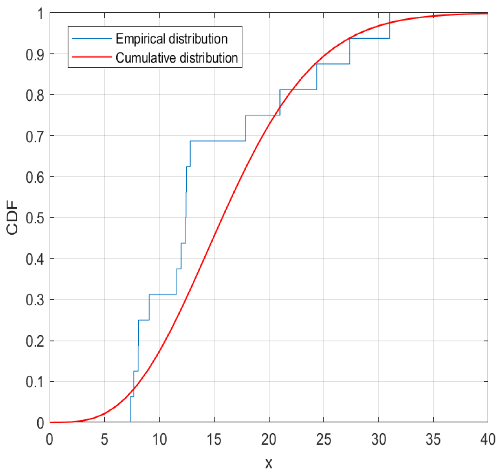
12.82, 17.86, 7.66, 12.48, 8.08, 7.35, 11.99, 21.00, 27.36, 8.11, 24.35, 12.44, 12.40, 31.01, 9.09, 11.57. In order to further analyze whether the obtained censored data also fit G R D ( σ , β ) , we drew an empirical distribution function graph under the censored data, and compared it with a G R D ( σ , β ) cumulative distribution function graph. Through image visualization, we can conclude that the censored data can reasonably fit the distribution (see Figure 2).
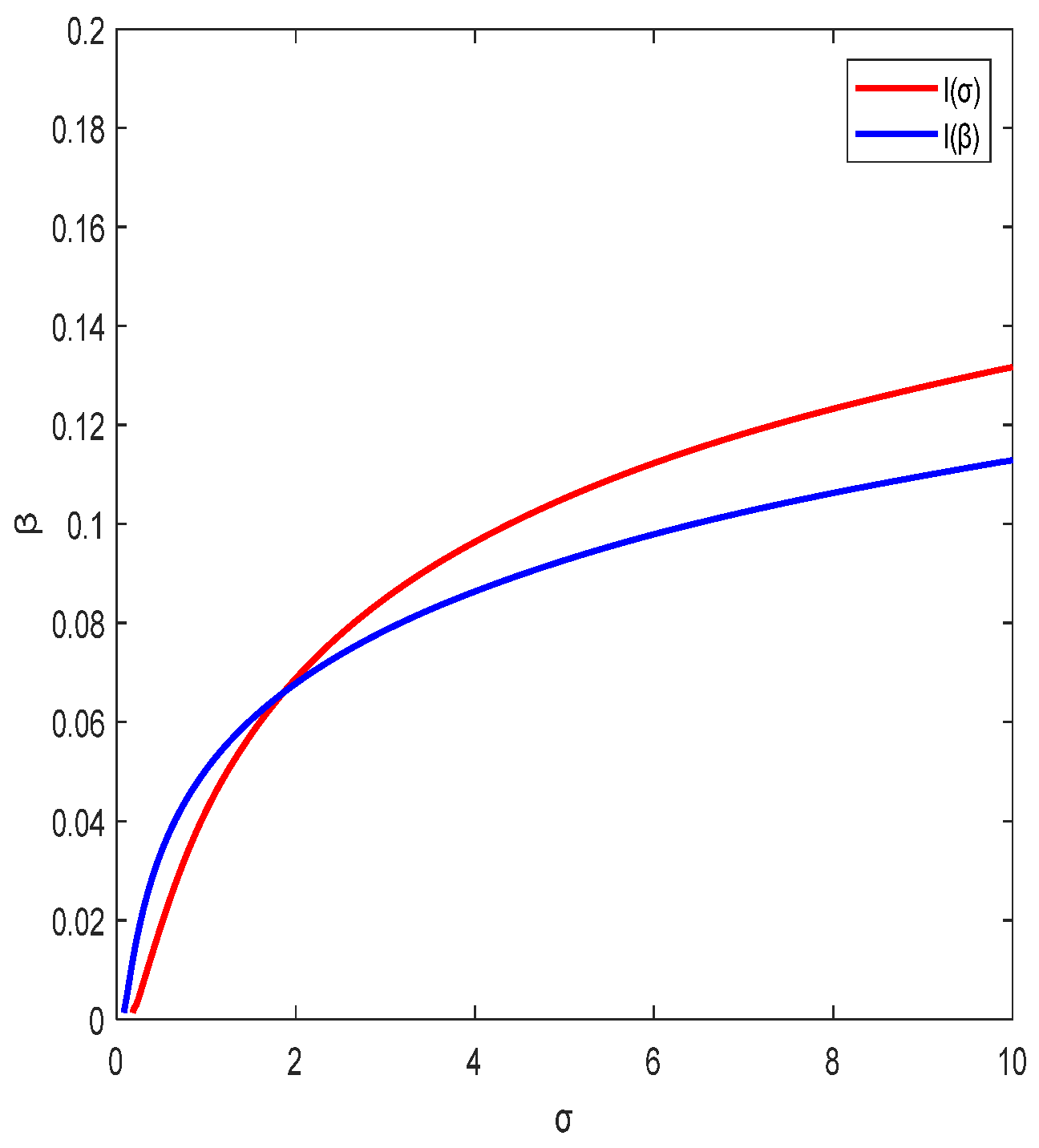
Before calculating real data, it is necessary to explain the existence and uniqueness of the ML estimation solution. Due to Equations (8) and (9) being nonlinear, proving them directly would be complex. Let us consider Equations (8) and (9); they are visually represented through the image shown in Figure 3, where l ( σ ) represents l ( σ , β ) σ in Equation (8) and l ( β )  represents  in Equation (9).
From Figure 3, we find that the two curves only have one intersection point, so we conclude that the solution for the ML estimation exists and is unique.
The estimation method described in this article was used to perform ML estimation and Bayesian estimation on the real data mentioned above and obtain parameters σ = 1.7051 ,   β = 0.0665 using real data; the specific results are shown in the Table 4.

6. Conclusions

This paper first described the G R D ( σ , β ) model and briefly outlined the characteristics of the model. Under the PC-II scheme, the Shannon entropy function obeying the G R D ( σ , β ) was derived, and the ML estimates of parameters were derived using the numerical Newton iterative method. In order to understand the reliability and stability of the obtained entropy estimation, the Delta method was subsequently used to obtain the ACI of entropy. In order to better choose the estimation method, Bayesian estimation was used to continue estimating the Shannon entropy function. This paper discussed the BEs of three loss functions: the WSELF, PLF, and KLF. Because the BEs under the above three loss functions were in the form of two integral ratios, which are complex to calculate, we chose Lindley’s approximation to obtain the Bayesian estimates of the entropy under the loss function. Finally, a Monte Carlo simulation was used to obtain the ML estimates and Bayesian estimate of MSE and CV. When the number of observed faults was fixed, MSE showed an upward trend as the sample size increased; when the sample size was fixed, as the number of observed faults increased, MSE showed a decreasing trend, and a higher CV indicated that the estimated results tended to be more realistic parameter values. Through the simulation in Section 5, it can be concluded that the performance of Bayesian estimation was superior to ML estimation, and the overall performance of the MCMC method was superior to Lindley’s approximation method.
The G R D ( σ , β ) model is one of the relatively new probability distribution models, and there is relatively little research on the estimation of the entropy of G R D ( σ , β ) . It was very meaningful to focus on the estimation of the entropy of G R D ( σ , β ) in this paper, which not only provided new ideas and methods for the estimation of the entropy of G R D ( σ , β ) , but also provides a deep understanding of the characteristics of the entropy of G R D ( σ , β ) , and promotes the research and development of related theories.

Author Contributions

Conceptualization, H.R. and Q.G.; methodology, H.R.; software, Q.G. and X.H.; validation, H.R. and X.H.; writing—original draft preparation, Q.G.; writing—review and editing, H.R.; funding acquisition, H.R. All authors have read and agreed to the published version of the manuscript.

Funding

This research was funded by the National Natural Science Foundation of China, grant number 71661012.

Data Availability Statement

Not applicable.

Conflicts of Interest

The authors declare no conflict of interest.

Appendix A

According to Equation (1), we can obtain
ln f ( x ) = ln [ 2 σ β 2 x e β 2 x 2 ( 1 e β 2 x 2 ) σ 1 ] = ln 2 σ β 2 + ln x β 2 x 2 + ( σ 1 ) ln ( 1 e β 2 x 2 ) ,
H ( f ) = 0 f ( x ) [ ln 2 σ β 2 + ln x β 2 x 2 + ( σ 1 ) ln ( 1 e β 2 x 2 ) ] d x = ln 2 σ β 2 0 f ( x ) d x 0 ln x f ( x ) d x + 0 β 2 x 2 f ( x ) d x 0 ( σ 1 ) ln ( 1 e β 2 x 2 ) f ( x ) d x = ln 2 σ β 2 E [ ln x ] + E [ β 2 x 2 ] ( σ 1 ) E [ ln ( 1 e β 2 x 2 ) ] .
Obviously, 0 f ( x ) d x = 1 ; that is
0 2 σ β 2 x e β 2 x 2 ( 1 e β 2 x 2 ) σ 1 d x = 1
At this point, both sides simultaneously align the σ derivative; we have
0 2 β 2 x e β 2 x 2 ( 1 e β 2 x 2 ) σ 1 d x + 0 2 σ β 2 x e β 2 x 2 ( 1 e β 2 x 2 ) σ 1 ln ( 1 e β 2 x 2 ) d x = 0
Therefore,
0 2 σ β 2 x e β 2 x 2 ( 1 e β 2 x 2 ) σ 1 ln ( 1 e β 2 x 2 ) = 1 σ
Hence,
E [ ln ( 1 e β 2 x 2 ) ] = 1 σ
Next, we can calculate that
E [ β 2 x 2 ] = 0 β 2 x 2 ( 2 σ β 2 x e β 2 x 2 ( 1 e β 2 x 2 ) σ 1 ) d x = 0 σ ( β 2 x 2 ) e β 2 x 2 ( 1 e β 2 x 2 ) σ 1 d ( β 2 x 2 ) .
Let β 2 x 2 = w ; then,
E [ w ] = 0 σ w e w ( 1 e w ) σ 1 d w
We know that the PDF of the generalized exponential distribution is
f ( v ) = β σ e v σ ( 1 e v σ ) β 1 ,
and know that [13] the following is true:
E ( v ) = 0 σ β v σ e v β ( 1 e v β ) β 1 d ( v σ ) = σ 0 β v σ e v β ( 1 e v β ) β 1 d ( v σ ) = σ [ ψ ( λ + 1 ) ψ ( 1 ) ] ,
that is to say
0 β v σ e v β ( 1 e v β ) β 1 d ( v σ ) = [ ψ ( β + 1 ) ψ ( 1 ) ]
Let v σ = w ; then,
0 β w e w ( 1 e w ) β 1 d w = [ ψ ( β + 1 ) ψ ( 1 ) ]
Thus,
E [ w ] = 0 σ w e w ( 1 e w ) σ 1 d w = [ ϕ ( σ + 1 ) ϕ ( 1 ) ]
We can calculate that
E ( x r ) = 0 x r f ( x ) d x = 0 x r 2 σ β 2 x e β 2 x 2 ( 1 e β 2 x 2 ) σ 1 d x = 0 σ x r e β 2 x 2 ( 1 e β 2 x 2 ) σ 1 d ( β 2 x 2 ) .
Let β 2 x 2 = t ; then, x = 1 β t 1 2 . Thus,
0 σ x r e β 2 x 2 ( 1 e β 2 x 2 ) σ 1 d ( β 2 x 2 ) = 0 σ ( 1 β t 1 2 ) r e t ( 1 e t ) σ 1 d t
= σ β r 0 t 1 2 e t ( 1 e t ) σ 1 d t .
Let e t = u ; then, t = ln u and d t = 1 u d u . Therefore,
σ β r 0 t 1 2 e t ( 1 e t ) σ 1 d t = σ β r 0 1 ( ln u ) r 2 ( 1 u ) σ 1 d u = σ β r 0 t 1 2 e t ( 1 e t ) σ 1 d t .
We can perform the polynomial decomposition of ( 1 u ) σ 1 to
( 1 u ) σ 1 = i = 0 ( σ 1 i ) ( 1 ) i u i
Then,
σ β r 0 1 ( ln u ) r 2 ( 1 u ) σ 1 d u = σ β r 0 1 ( ln u ) r 2 i = 0 ( σ 1 i ) ( 1 ) i u i d u = σ β r i = 0 ( σ 1 i ) ( 1 ) i 0 1 ( ln u ) r 2 u i d u
According to the negative logarithmic gamma distribution:
0 1 ( ln u ) r 2 ( 1 u ) σ 1 d u = Γ ( r 2 + 1 ) ( 1 + i ) r 2 + 1
Thus,
σ β r i = 0 ( σ 1 i ) ( 1 ) i 0 1 ( ln u ) r 2 u i d u = σ β r i = 0 ( σ 1 i ) ( 1 ) i Γ ( r 2 + 1 ) ( 1 + i ) r 2 + 1
E [ x r ] = σ β r i = 0 ( σ 1 i ) ( 1 ) i Γ ( r 2 + 1 ) ( 1 + i ) r 2 + 1
d E [ x r ] d r = E [ x r ln x ] = σ β r ln β i = 0 ( σ 1 i ) ( 1 ) i Γ ( r 2 + 1 ) ( 1 + i ) r 2 + 1 + σ β r i = 0 ( σ 1 i ) ( 1 ) i Γ ( r 2 + 1 ) 1 2 ( 1 + i ) r 2 + 1 Γ ( r 2 + 1 ) ( 1 + i ) r 2 + 1 1 2 ln ( 1 + i ) ( 1 + i ) r + 2
If r = 0 , then
E [ ln x ] = σ ln β i = 0 ( σ 1 i ) ( 1 ) i Γ ( 1 ) ( 1 + i ) + σ i = 0 ( σ 1 i ) ( 1 ) i 1 2 Γ ( 1 ) 1 2 Γ ( 1 ) ln ( 1 + i ) ( 1 + i )
= σ i = 0 ( σ 1 i ) ( 1 ) i 1 2 Γ ( 1 ) Γ ( 1 ) ln [ β ( 1 + i ) 1 2 ] 1 + i
Thus,
H s ( f ) = ln 2 σ β 2 σ i = 0 ( σ 1 i ) ( 1 ) i 1 2 Γ ( 1 ) Γ ( 1 ) ln [ β ( 1 + i ) 1 2 ] 1 + i + [ ϕ ( σ + 1 ) ϕ ( 1 ) ] 1 σ + 1
Hence, the proof of Theorem 1 is completed.

References

  1. Kundu, D.; Raqab, M.Z. Generalized Rayleigh distribution: Different methods of estimations. Comput. Stat. Data Anal. 2005, 49, 187–200. [Google Scholar] [CrossRef]
  2. Surles, J.G.; Padgett, W.J. Inference for reliability and stress-strength for a scaled Burr Type X distribution. Lifetime Data Anal. 2001, 7, 187–200. [Google Scholar] [CrossRef]
  3. Yan, W.A.; Li, P.; Yu, Y.X. Statistical inference for the reliability of Burr-XII distribution under improved adaptive Type-II progressive censoring. Appl. Math. Model. 2021, 95, 38–52. [Google Scholar] [CrossRef]
  4. Jamal, F.; Chesneau, C.; Nasir, M.A.; Saboor, A.; Altun, E.; Khan, M.A. On a modified Burr XII distribution having flexible hazard rate shapes. Math. Slovaca 2020, 70, 193–212. [Google Scholar] [CrossRef]
  5. Chang, H.; Ding, J.J.; Wu, L.N. Performance of EBPSK demodulator in AWGN channel. J. Southeast Univ. Natural Sci. 2012, 42, 14–19. [Google Scholar]
  6. Fu, R.L.; Ma, Y.X.; Dong, G.H. Researches on statistical properties of freak waves in uni-directional random waves in deep water. Acta Oceanologica Sin. 2021, 43, 81–89. [Google Scholar]
  7. Feng, Y.; Song, S.; Xu, C.Q. Two-parameter generalized Rayleigh distribution. Math. Appl. 2022, 35, 128–136. [Google Scholar]
  8. Çolak, A.B.; Sindhu, T.N.; Lone, S.A.; Shafiq, A.; Abushal, T.A. Reliability study of generalized Rayleigh distribution based on inverse power law using artificial neural network with Bayesian regularization. Tribol. Int. 2023, 185, 108544. [Google Scholar] [CrossRef]
  9. Shen, B.L.; Chen, W.X.; Wang, S.; Chen, M. Fisher information for generalized Rayleigh distribution in ranked set sampling design with application to parameter estimation. Appl. Math. Ser. B 2022, 37, 615–630. [Google Scholar] [CrossRef]
  10. Shen, Z.J.; Alrumayh, A.; Ahmad, Z.; Abu-Shanab, R.; Al-Mutairi, M.; Aldallal, R. A new generalized rayleigh distribution with analysis to big data of an online community. Alex. Eng. J. 2022, 61, 11523–11535. [Google Scholar] [CrossRef]
  11. Rabie, A.; Hussam, E.; Muse, A.H.; Aldallal, R.A.; Alharthi, A.S.; Aljohani, H.M. Estimations in a constant-stress partially accelerated life test for generalized Rayleigh distribution under Type-II hybrid censoring scheme. J. Math.-UK 2022, 2022, 6307435. [Google Scholar] [CrossRef]
  12. Raqab, M.Z.; Kundu, D. Burr Type X distribution: Revisited. J. Probab. Stat. Sci. 2006, 4, 179–193. [Google Scholar]
  13. Xu, R.; Gui, W.H. Entropy estimation of inverse Weibull distribution under Adaptive Type-II progressive hybrid censoring schemes. Symmetry 2019, 11, 1463. [Google Scholar]
  14. Chacko, M.; Asha, P.S. Estimation of entropy for generalized exponential distribution based on record values. J. Indian Soc. Prob. St. 2018, 19, 79–96. [Google Scholar] [CrossRef]
  15. Shrahili, M.; El-Saeed, A.R.; Hassan, A.S.; Elbatal, I.; Elgarhy, M. Estimation of entropy for Log-Logistic distribution under progressive Type-II censoring. J. Nanomater. 2022, 2022, 2739606. [Google Scholar] [CrossRef]
  16. Wang, X.J.; Gui, W.H. Bayesian estimation of entropy for Burr type XII distribution under progressive Type-II censored data. Mathematics 2021, 9, 313. [Google Scholar] [CrossRef]
  17. Al-Babtain, A.A.; Elbatal, I.; Chesneau, C.; Elgarhy, M. Estimation of different types of entropies for the Kumaraswamy distribution. PLoS ONE 2021, 16, e0249027. [Google Scholar] [CrossRef] [PubMed]
  18. Bantan, R.A.R.; Elgarhy, M.; Chesneau, C.; Jamal, F. Estimation of entropy for inverse Lomax distribution under multiple censored data. Entropy 2020, 22, 601. [Google Scholar] [CrossRef]
  19. Shi, X.L.; Shi, Y.M.; Zhou, K. Estimation for entropy and parameters of generalized Bilal distribution under adaptive Type-II progressive hybrid censoring scheme. Entropy 2021, 23, 206. [Google Scholar] [CrossRef] [PubMed]
  20. Liu, S.H.; Gui, W.H. Estimating the entropy for Lomax distribution based on generalized progressively hybrid censoring. Symmetry 2019, 11, 1219. [Google Scholar] [CrossRef] [Green Version]
  21. Zhou, X.D.; Qi, X.R.; Yue, R.X. Statistical analysis for Type-II progressive interval censored data based on Weibull survival regression models. J. Syst. Sci. Math. Sci. Chin. Ser. 2023, 43, 1346–1361. [Google Scholar]
  22. Almarashi, A.; Abd-Elmougod, G. Accelerated competing risks model from Gompertz lifetime distributions with Type-II censoring scheme. Therm. Sci. 2020, 24, 165–175. [Google Scholar] [CrossRef]
  23. Ramadan, D.A. Assessing the lifetime performance index of weighted Lomax distribution based on progressive Type-II censoring scheme for bladder cancer. Int. J. Biomath. 2022, 14, 2150018. [Google Scholar] [CrossRef]
  24. Hashem, A.F.; Alyami, S.A. Inference on a new lifetime distribution under progressive Type-II censoring for a parallel-series structure. Complexity 2021, 2021, 6684918. [Google Scholar] [CrossRef]
  25. Luo, C.L.; Shen, L.J.; Xu, A.C. Modelling and estimation of system reliability under dynamic operating environments and lifetime ordering constraints. Reliab. Eng. Syst. Saf. 2022, 218, 108136. [Google Scholar] [CrossRef]
  26. Ren, J.; Gui, W. Statistical analysis of adaptive Type-II progressively censored competing risks for Weibull models. Appl. Math. Model. 2021, 98, 323–342. [Google Scholar] [CrossRef]
  27. Zhou, S.R.; Xu, A.C.; Tang, Y.C.; Shen, L.J. Fast Bayesian inference of reparameterized Gamma process with random effects. IEEE Trans. Reliab. 2023, 1–14. [Google Scholar] [CrossRef]
  28. Zhuang, L.L.; Xu, A.C.; Wang, X.L. A prognostic driven predictive maintenance framework based on Bayesian deep learning. Reliab. Eng. Syst. Saf. 2023, 234, 109181. [Google Scholar] [CrossRef]
  29. Wang, X.; Song, L. Bayesian estimation of Pareto distribution parameter under entropy loss based on fixed time censoring data. J. Liaoning Tech. Univ. (Nat. Sci. Edit.) 2013, 32, 245–248. [Google Scholar]
  30. Renjini, K.R.; Abdul-Sathar, E.I.; Rajesh, G. A study of the effect of loss functions on the Bayes estimates of dynamic cumulative residual entropy for Pareto distribution under upper record values. J. Stat. Comput. Simul. 2016, 86, 324–339. [Google Scholar] [CrossRef]
  31. Han, M. E-Bayesian estimations of parameter and its evaluation standard: E-MSE (expected mean square error) under different loss functions. Commun Stat.-Simul. Comput. 2021, 50, 1971–1988. [Google Scholar] [CrossRef]
  32. Rasheed, H.A.; Abd, M.N. Bayesian Estimation for two parameters of exponential distribution under different loss functions. Ibn Al-Haitham J. Pure Appl. Sci. 2023, 36, 289–300. [Google Scholar] [CrossRef]
  33. Hassan, A.S.; Elsherpieny, E.A.; Mohamed, R.E. Classical and Bayesian estimation of entropy for Pareto distribution in presence of outliers with application. Sankhya A 2022, 85, 707–740. [Google Scholar] [CrossRef]
  34. Kohansal, A. On estimation of reliability in a multicomponent stress-strength model for a Kumaraswamy distribution based on progressively censored sample. Stat. Pap. 2019, 60, 2185–2224. [Google Scholar] [CrossRef]
  35. Luengo, D.; Martino, L.; Bugallo, M.; Elvira, V.; Särkkä, S. A survey of Monte Carlo methods for parameter estimation. Eurasip J. Adv. Signal Process. 2020, 2020, 101186. [Google Scholar] [CrossRef]
  36. Das, A.; Debnath, N. Sampling-based techniques for finite element model updating in bayesian framework using commercial software. Lect. Notes Civ. Eng. 2021, 81, 363–379. [Google Scholar]
  37. Karunarasan, D.; Sooriyarachchi, R.; Pinto, V. A comparison of Bayesian Markov chain Monte Carlo methods in a multilevel scenario. Commun. Stat.-Simul. Comput. 2021, 81, 1–17. [Google Scholar] [CrossRef]
  38. Raqab Mohammad, Z. Discriminating between the generalized Rayleigh and Weibull distributions. J. Appl. Stat. 2013, 40, 1480–1493. [Google Scholar] [CrossRef]
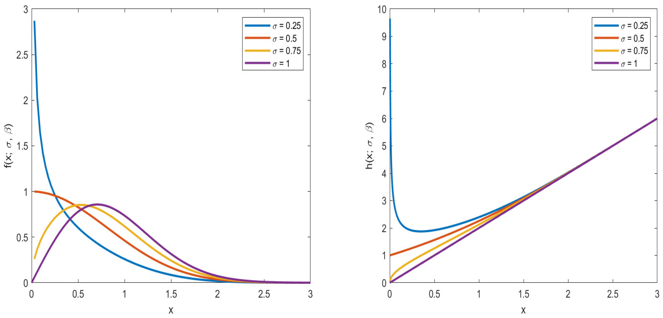
Figure 1. Curves of PDF and HF of the G R D ( σ , β ) .
Axioms 12 00776 g001
Figure 2. Empirical distribution under censored data and cumulative distribution function of G R D ( σ , β ) .
Axioms 12 00776 g002
Figure 3. Partial derivative of log-LF.
Axioms 12 00776 g003
Table 1. Censoring schemes.
Scheme
a P 1 = P 2 = = P m 1 = 0 , P m = n m
b P 1 = P 2 = P 3 = = P m = 1
c P 1 = n m , P 2 = = P m 1 = 0
Table 2. The ML estimates and Bayesian estimates of different censoring schemes (CSs) under the G R D ( σ , β ) and their corresponding MSEs (in parentheses).
MLELindleyMCMC
n m C S M M L M w M P M K M w M P M K
3010a
b
c
0.4103 (0.0951)
0.4354 (0.0721)
0.4868 (0.0503)
0.3930 (0.0977)
0.4144 (0.0753)
0.4599 (0.0548)
0.4568 (0.0665)
0.4698 (0.0514)
0.5141 (0.0296)
0.3173 (0.1125)
0.3252 (0.0923)
0.3651 (0.0799)
0.7545 (0.0498)
0.6278 (0.0052)
0.7792 (0.0500)
0.8294 (0.0749)
0.7333 (0.0315)
0.8092 (0.0643)
0.7788 (0.0749)
0.6621 (0.0113)
0.7891 (0.0544)
15a
b
c
0.4825 (0.0466)
0.4876 (0.0414)
0.5043 (0.0325)
0.4688 (0.0490)
0.4726 (0.0439)
0.4852 (0.0350)
0.4999 (0.0419)
0.5054 (0.0380)
0.5205 (0.0292)
0.3603 (0.0804)
0.3640 (0.0744)
0.3729 (0.0635)
0.6821 (0.0160)
0.6216 (0.0043)
0.6807 (0.0156)
0.7243 (0.0284)
0.6441 (0.0078)
0.7122 (0.0245)
0.6961 (0.0197)
0.6291 (0.0054)
0.6914 (0.0184)
20a
b
c
0.5044 (0.0290)
0.5100 (0.0313)
0.5083 (0.0243)
0.4926 (0.0305)
0.4987 (0.0327)
0.4946 (0.0256)
0.5159 (0.0278)
0.5214 (0.0298)
0.5207 (0.0234)
0.3739 (0.0609)
0.3783 (0.0623)
0.3737 (0.0545)
0.6649 (0.0119)
0.5896 (0.0011)
0.5670 (0.0002)
0.6827 (0.0161)
0.6142 (0.0034)
0.6121 (0.0032)
0.6708 (0.0132)
0.5976 (0.0018)
0.5841 (0.0008)
4010a
b
c
0.4130 (0.1044)
0.4483 (0.0722)
0.4870 (0.0452)
0.3955 (0.1702)
0.4267 (0.0751)
0.4590 (0.0495)
0.4631 (0.0757)
0.4866 (0.0533)
0.5121 (0.0330)
0.3289 (0.1196)
0.3413 (0.0971)
0.3614 (0.0739)
0.6840 (0.0165)
0.7307 (0.0306)
0.6416 (0.0074)
0.7163 (0.0258)
0.7932 (0.0564)
0.6936 (0.0190)
0.6949 (0.0194)
0.7524 (0.0387)
0.6593 (0.0107)
15a
b
c
0.4702 (0.0565)
0.4842 (0.0413)
0.5060 (0.0328)
0.4574 (0.0583)
0.4693 (0.0435)
0.4873 (0.0351)
0.4910 (0.0495)
0.5015 (0.0376)
0.5223 (0.0303)
0.3533 (0.0881)
0.3597 (0.0743)
0.3731 (0.0633)
0.6292 (0.0054)
0.6748 (0.0142)
0.5874 (0.0010)
0.6587 (0.0106)
0.6919 (0.0186)
0.6208 (0.0042)
0.6391 (0.0069)
0.6807 (0.0156)
0.5984 (0.0018)
20a
b
c
0.4934 (0.0332)
0.5077 (0.0313)
0.5201 (0.0249)
0.4829 (0.0346)
0.4964 (0.0330)
0.5066 (0.0264)
0.5049 (0.0315)
0.5193 (0.0299)
0.5324 (0.0234)
0.3645 (0.0658)
0.3759 (0.0662)
0.3861 (0.0557)
0.6097 (0.0030)
0.6580 (0.0105)
0.5681 (0.0002)
0.6329 (0.0060)
0.6880 (0.0175)
0.5948 (0.0015)
0.6174 (0.0038)
0.6680 (0.0126)
0.5772 (0.0005)
5015a
b
c
0.4728 (0.0611)
0.4860 (0.0470)
0.5160 (0.0257)
0.4610 (0.0630)
0.4709 (0.0494)
0.4975 (0.0277)
0.4926 (0.0542)
0.5042 (0.0403)
0.5319 (0.0241)
0.3562 (0.0931)
0.3629 (0.0782)
0.3840 (0.0565)
0.6316 (0.0058)
0.6450 (0.0080)
0.6145 (0.0035)
0.6636 (0.0116)
0.6739 (0.0140)
0.6757 (0.0144)
0.6422 (0.0075)
0.6543 (0.0097)
0.6341 (0.0061)
20a
b
c
0.4929 (0.0391)
0.5058 (0.0316)
0.5205 (0.0217)
0.4832 (0.0403)
0.4946 (0.0330)
0.5069 (0.0232)
0.5056 (0.0372)
0.5176 (0.0296)
0.5329 (0.0200)
0.3687 (0.0707)
0.3752 (0.0634)
0.3865 (0.0515)
0.6039 (0.0023)
0.6432 (0.0077)
0.6048 (0.0024)
0.6260 (0.0049)
0.6528 (0.0094)
0.6559 (0.0100)
0.6112 (0.0031)
0.6465 (0.0082)
0.6215 (0.0043)
30a
b
c
0.5222 (0.0209)
0.5236 (0.0175)
0.5265 (0.0168)
0.5147 (0.0216)
0.5162 (0.0180)
0.5174 (0.0176)
0.5294 (0.0203)
0.5310 (0.0172)
0.5346 (0.0164)
0.3884 (0.0527)
0.3876 (0.0456)
0.3891 (0.0464)
0.5792 (0.0006)
0.5778 (0.0005)
0.5769 (0.0004)
0.5921 (0.0013)
0.5910 (0.0012)
0.5909 (0.0011)
0.5836 (0.0008)
0.5822 (0.0007)
0.5816 (0.0006)
Table 3. Lower 100 (1 − α)% coverage and variance with different α.
n m C S α   =   0.1 α   =   0.05 V ( H ^ ( f ) )
3010a
b
c
0.7480
0.8240
0.9110
0.7160
0.7480
0.8750
0.0219
0.0095
0.0149
15a
b
c
0.8110
0.8560
0.9170
0.7650
0.7950
0.8590
0.0063
0.0076
0.0135
20a
b
c
0.8570
0.8880
0.8940
0.7960
0.8090
0.8740
0.0064
0.0069
0.0089
4010a
b
c
0.7290
0.8220
0.9230
0.6970
0.7510
0.8820
0.0090
0.0219
0.0112
15a
b
c
0.7930
0.8420
0.9100
0.7240
0.7700
0.8770
0.0069
0.0087
0.0171
20a
b
c
0.8390
0.8310
0.9190
0.7690
0.8270
0.8780
0.0044
0.0037
0.0070
5015a
b
c
0.7620
0.8510
0.9410
0.7160
0.8020
0.8880
0.0030
0.0107
0.0099
20a
b
c
0.8060
0.8590
0.9200
0.7530
0.8120
0.8950
0.0040
0.0055
0.0061
30a
b
c
0.8520
0.8720
0.9270
0.7810
0.8300
0.8810
0.0050
0.0028
0.0052
Table 4. Estimates of Shannon entropy.
ML EstimatesBayesian Estimates
LindleyMCMC
under WSEKFunder PLFunder KLFunder WSEKFunder PLFunder KLF
3.28153.27043.28445.93483.16493.17373.1678
Disclaimer/Publisher’s Note: The statements, opinions and data contained in all publications are solely those of the individual author(s) and contributor(s) and not of MDPI and/or the editor(s). MDPI and/or the editor(s) disclaim responsibility for any injury to people or property resulting from any ideas, methods, instructions or products referred to in the content.