Article

The Laplace Transform Shortcut Solution to a One-Dimensional Heat Conduction Model with Dirichlet Boundary Conditions

1
School of Urban Construction and Transportation, Hefei University, Hefei 230601, China
2
School of Civil Engineering, Hefei University of Technology, Hefei 230009, China
*
Author to whom correspondence should be addressed.
Axioms 2023, 12(8), 770; https://doi.org/10.3390/axioms12080770
Submission received: 20 June 2023 / Revised: 18 July 2023 / Accepted: 7 August 2023 / Published: 9 August 2023
(This article belongs to the Special Issue Differential Equations and Inverse Problems)

Abstract

:
When using the Laplace transform to solve a one-dimensional heat conduction model with Dirichlet boundary conditions, the integration and transformation processes become complex and cumbersome due to the varying properties of the boundary function f(t). Meanwhile, if f(t) has a complex functional form, e.g., an exponential decay function, the product of the image function of the Laplace transform and the general solution to the model cannot be obtained directly due to the difficulty in solving the inverse. To address this issue, operators are introduced to replace f(t) in the transformation process. Based on the properties of the Laplace transform and the convolution theorem, without the direct involvement of f(t) in the transformation, a general theoretical solution incorporating f(t) is derived, which consists of the product of erfc(t) and f(0), as well as the convolution of erfc(t) and the derivative of f(t). Then, by substituting f(t) into the general theoretical solution, the corresponding analytical solution is formulated. Based on the general theoretical solution, analytical solutions are given for f(t) as a commonly used function. Finally, combined with an exemplifying application demonstration based on the test data of temperature T(x, t) at point x away from the boundary and the characteristics of curve T(x, t) − t and curve 𝜕T(x, t)/𝜕tt, the inflection point and curve fitting methods are established for the inversion of model parameters.

1. Introduction

The one-dimensional heat conduction model in a half-infinite domain with Dirichlet boundary conditions is a classical heat conduction model [1]. In this model, the boundary function f(t) is assumed to be a known constant ΔT0 (representing an instantaneous change ΔT0 in the initial temperature and remaining constant). An analytical solution for the model can be directly obtained using Laplace and Fourier transforms [1,2,3].
In practical problems, the expression of f(t) is often complex and variable. As the boundary function type of f(t) changes or the same function type has different expressions, complex and tedious integral transform operations are needed to obtain the solution to the problem [3]. For some complex boundary functions, specific solution methods have been proposed, such as the thermal equilibrium integral method [4,5,6,7] and the boundary value method [8,9]. To effectively deal with complex and varied boundary functions, some of the literature has extensively investigated the impact of boundary conditions on model solutions [10], as well as methods for handling boundaries in specific problems [10,11,12,13,14]. Among the studies of similar problems based on the one-dimensional heat conduction model, such as groundwater seepage in a semi-infinite aquifer under the control of river and channel boundaries, the literature [15,16,17,18,19,20,21,22] provides a detailed investigation of a seepage model under changing river and channel water level characteristics. The solution methods in these studies are too complex, making their application difficult, or the treatment of boundary conditions is difficult to generalize in practical applications. However, there are still cases where the model is difficult to solve directly when common function types are used as boundary functions in one-dimensional heat conduction models. For instance, when f(t) is an exponentially decaying function ∆T0 e−λt after the Laplace transform, the inverse problem of the combined product of the model’s general solution and the function-like f(t) becomes difficult to solve directly.
In practical problems, the function type of f(t) is complex and variable [20,21]. To avoid the complex and tedious process of integral transform operations mentioned above, the literature [21] proposed a shortcut Fourier transform method for f(t) as the Lagrange linear interpolation equation when solving unsteady-flow models near river and canal boundaries. This method exploits the properties of the Fourier transform and the convolution theorem, enabling f(t) to participate in the transformation process indirectly. When f(t) is an exponentially decaying function, the one-dimensional heat conduction model is difficult to solve directly using Laplace and Fourier transforms. To address this problem, research on the fast solution method based on the feature that f(t) does not directly participate in the transformation process is carried out in the literature [22,23].
The shortcut solution for the Laplace and Fourier transforms provides a general theoretical solution approach for models of this type by replacing f(t) with operators and performing calculations in the transformation process without directly computing the transformation of f(t). This approach is based on the differential properties of the transform and the convolution theorem. Given the conditions for determining f(t) in practical problems, the general theoretical solution is applied by substituting f(t) to obtain the actual solution to the problem [19,20,21]. This solving approach does not need complex and cumbersome integral transformation processes, making it a fast, concise, and convenient alternative to traditional solving methods.
This paper systematically describes the process of establishing the Laplace transform shortcut solution method and provides the analytical solutions of several common function types using the general theoretical solution. Combined with the exemplifying research, the establishment and application of the inflection point and curve fitting methods for calculating model parameters using temperature-based dynamic monitoring data are demonstrated.

2. Basic Model

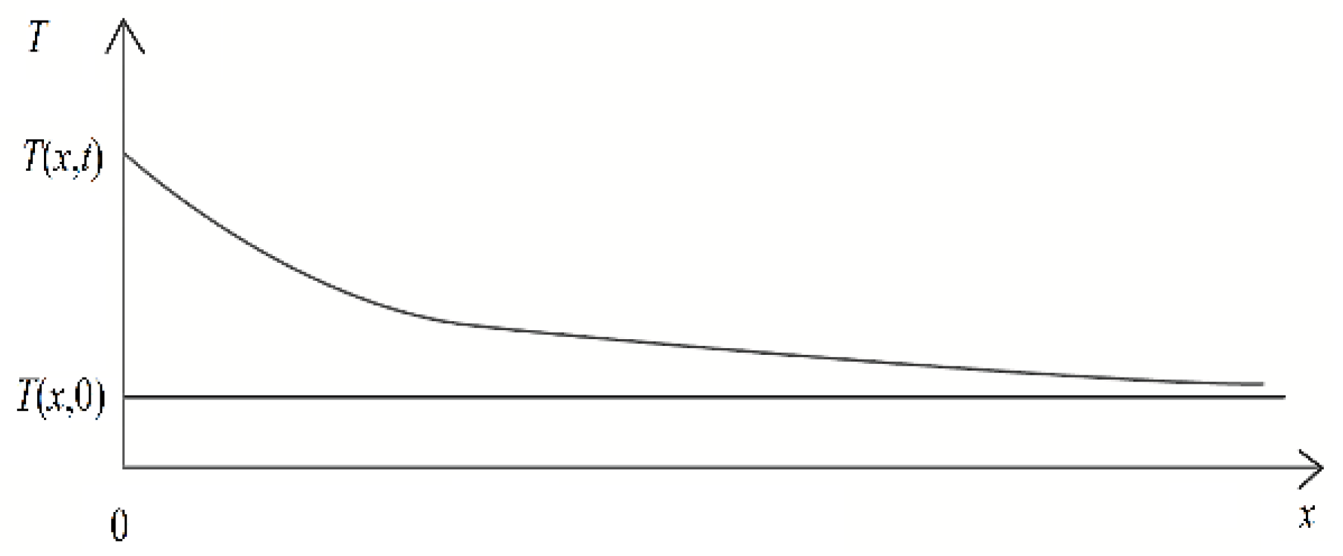
As illustrated in Figure 1 and Figure 2, the one-dimensional heat conduction problem in the semi-infinite domain under Dirichlet boundary control assumes:
(1)
A homogeneous thin plate extending infinitely in the x-direction, with a heat source at the boundary (x = 0) that varies with time as f(t). f(t) must meet the basic requirements of the Laplace transform.
(2)
The temperature at any point within the thin plate can be represented as T(x, t), and the initial temperature is uniformly zero: T(x, 0) = 0.
(3)
The outer surface of the thin plate is insulated, indicating that there is no heat exchange between the thin plate and the external environment, and the one-dimensional heat conduction only occurs within the thin plate due to the boundary heat source.
The above problem can be represented as a mathematical model (I):
T t = a 2 T x 2 ( 0 < x < + , t > 0 ) ,
T ( x ,   t ) | t = 0 = T ( x ,   0 ) ( x > 0 ) ,
T ( x ,   t ) | x = 0 = T ( 0 , 0 ) + f ( t ) ( t 0 ) ,
where a (m2/s) represents the thermal diffusivity or thermal conductivity of the solid material.

3. General Theoretical Solution

By defining u(x, t) = T(x, t) − T(x, 0), the mathematical model (I) can be rewritten as (II):
u t = a 2 u x 2 ( 0 < x < + ,   t > 0 ) ,
u ( x ,   t ) | t = 0 = 0 ( x > 0 ) ,
u ( x ,   t ) | x = 0 = f ( t ) ( t 0 ) ,
The right end of Formula (5) is 0, which is convenient for the later formula derivation and expression simplification.
Taking the Laplace transform of model (II) with respect to t yields model (III):
d 2 u ¯ d x 2 s D u ¯ = 0 ,
u ¯ | x = 0 = L [ f ( t ) ] ,
where u ¯ represents the Laplace transform of u with respect to t, s is the Laplace operator, and L and L−1 denote the Laplace transform operator and the inverse transform operator, respectively.
In the aforementioned process, during the transformation of boundary condition (6) to boundary condition (8), f(t) does not directly participate in the transformation process. That is, the transformation operation does not involve calculating the image function of f(t). Instead, f(t) is treated as an operator in the direct transformation process.
The general solution to Equation (7) in Part (III) is
u ¯ ( x , s ) = c 1 exp ( s a x ) + c 2 exp ( s a x ) ,
where c1 and c2 are undetermined constants. With the boundary conditions (8), considering the mathematical meaning of the solution as x approaches infinity ( u ( x , t ) | x = 0 , U ¯ | x = 0 ), the specific solution for model (III) is
u ¯ ( x , s ) = L [ f ( t ) ] exp ( s a x ) ,
Applying the inverse Laplace transform to Equation (10) yields the solution to the problem. When the Laplace transform is used to solve the one-dimensional heat conduction model, the image function of L[f(t)] is usually obtained and substituted into Equation (10). Then, the inverse Laplace transform is applied to Equation (10), and the solution to the problem can be obtained.
When the form of f(t) is complicated or f(t) is of a special function type, it is difficult to find the solution to the problem using the above method. If f(t) is an exponentially decaying function ∆T0 eλt, where λ > 0, and the image function of L[f(t)] is ∆T0/(s + λ), the right-hand side of the above Equation becomes Δ T 0 exp ( s / a x ) / ( s + λ ) . The convolution of this product combination during the inverse transformation makes it challenging to obtain the solution directly [3]. Therefore, it is difficult to obtain the solution to the problem by directly using the Laplace transform.
To avoid the above tedious or even solution-free inverse process, under the condition that the image function of f(t) is not sought and the inverse of the product of the image function and the general solution is not sought, L[f(t)] is used as an operator on the Laplace inverse transform process to establish the Laplace transform general theoretical solution, provided that f(t) satisfies the basic requirements of the Laplace transform.
According to the “convolution theorem for Laplace inversions” [3], we have
u ( x , t ) = L 1 [ u ¯ ( x , s ) ] = L 1 [ L ( f ( t ) ) exp ( s a x ) ] , = L 1 [ L ( f ( t ) ) ] L 1 [ exp ( s a x ) ] = f ( t ) L 1 [ exp ( s a x ) ] ,
where represents the convolution operator.
The inverse Laplace transform function of the complementary error function “erfc(u)” [3] is
L 1 [ 1 s exp ( s a x ) ] = 2 π x 2 a t + e ζ 2 d ζ = e r f c ( x 2 a t ) ,
The left-hand side L 1 [ 1 s exp ( s a x ) ] of Equation (12) and the right-hand side L 1 [ exp ( s a x ) ] of Equation (11) have a differential relationship in the context of the inverse Laplace transform. For Equation (11), according to the “differential property” of the inverse Laplace transform [3], we have
L 1 [ exp ( s a x ) ] = L 1 { s [ 1 s exp ( s a x ) ] } = d d t { L 1 [ 1 s exp ( s a x ) ] } ,
Substituting Equation (12) into (13) yields
L 1 [ exp ( s a x ) ] = d d t [ e r f c ( x 2 a t ) ]
Substituting Equation (14) into (11) yields
u ( x , t ) = L 1 [ u ¯ ( x , s ) ] = L 1 [ L ( f ( t ) ) ] L 1 [ exp ( s a x ) ] = f ( t ) d d t [ e r f c ( x 2 a t ) ] ,
The “convolution differentiation” [3] property of the Laplace transform implies that
f ( t ) d d t [ e r f c ( x 2 a t ) ] + f ( t ) [ e r f c ( x 2 a t ) | t = 0 ] = e r f c ( x 2 a t ) d [ f ( t ) ] d t + f ( t ) | t = 0 e r f c ( x 2 a t ) ,
Because e r f c ( x 2 a t ) | t = 0 = 0 , through Equations (15) and (16), after rearrangement, we have
u ( x , t ) = f ( t ) d d t [ e r f c ( x 2 a t ) ] , = f ( t ) | t = 0 e r f c ( x 2 a t ) + e r f c ( x 2 a t ) d [ f ( t ) ] d t ,
Note that u(x, t) = T(x, t) − T(x, 0) and T(x, 0) = 0. According to the commutative property of convolution, the above Equation can be written in the following integral form:
T ( x , t ) = f ( t ) | t = 0 e r f c ( x 2 a t ) + 0 t d [ f ( t ) ] d t e r f c ( x 2 a ( t τ ) ) d τ .
Equation (18) represents a model solution obtained under the condition that f(t) is not directly involved in the transformation process. The solution contains f(t). It is worth noting that T(x, 0) = 0, but f(0) is not necessarily equal to 0. In practical applications, it is necessary to substitute the known f(t) and further expand the Equation to obtain the solution to the actual problem. Therefore, for any given f(t), Equation (18) represents the general theoretical solution of the model.

4. Solution for Boundary Functions of Commonly Used Function Types

Based on the general theoretical solution, this paper provides solutions for boundary functions of commonly used function types for ease of reference in practical applications.
In engineering and technology, commonly used function types include constant functions, polynomial functions, and elementary functions.

4.1. Constant Function

A constant function indicates that f(t) is a constant, and f(t) = ∆T0. The physical significance of this condition is that as t approaches 0+, the boundary temperature undergoes an instantaneous change of ∆T0 and remains constant after that. This constitutes the classical one-dimensional heat conduction model.
In this case, based on Equation (18), we have d[f(t)]/dt = d[∆T0]/dt = 0 and f(0) = ∆T0, which leads to
T ( x , t ) = Δ T 0 e r f c ( x 2 a t ) .
Equation (19) is the solution to the classical model [1,2,3].

4.2. Linear Interpolation Function

For the one-dimensional heat conduction problem with Dirichlet boundary conditions, although many variables vary continuously with time, actual observation processes are often discrete. For example, boundary temperature measurement data, even self-recorded test data, are mostly collected at a certain time interval from the previous test, so it is necessary to make extractions. Therefore, to express the variations in variables over time based on discrete measured data, piecewise function types are commonly used [24].
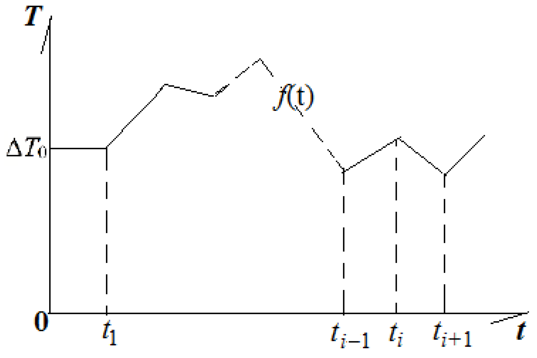
When a variable has a complex variation process, it is common to discretize f(t) based on the measured data using methods such as linear interpolation, including the Lagrange linear interpolation equation.
f ( t ) = Δ T 0 + i = 2 n [ f ( t i ) f ( t i 1 ) ] t t i 1 t i t i 1 δ ( t t i 1 ) .
where δ(tti−1) is the Heaviside function and has the following properties [25]: when t < ti1, δ(tti−1) = 0, and when t ≥ ti−1, δ(tti−1) = 1.
Substituting Equation (20) into (18), considering the properties of the δ(tti−1) function, we have
T ( x , t ) = Δ T 0 e r f c ( x 2 a t ) + i = 2 n f ( t i ) f ( t i 1 ) t i t i 1 t i 1 t e r f c ( x 2 a t ) d t .
Note that ∆T0 represents the interval during which the temperature remains constant starting from t→0+, and this constant period is from t1 to t0 (Figure 3). Therefore, the summation part in Equation (20) is for i = 2 − n. When establishing an interpolation equation for f(t) based on the definition of ∆T0, it is important to consider the expression of each time interval in the function [26].

4.3. Step Function

For the boundary temperature f(ti, ti+1) in the segment between titi+1(i ≥ 2), the average value of the temperature [f(ti) + f(ti+1)]/2 in the time period is used, or the increase f(ti+1) − f(ti) in the time period after t1 is used. The step function of f(t) can be written as
f ( t ) = Δ T 0 + i = 2 n [ ( f ( t i ) f ( t i 1 ) ] δ ( t t i 1 ) ( t > t i 1 , i N * ) ,
Substituting Equation (22) into (18), considering the properties of δ(tti−1) and f(0)= ∆T0, we have
T ( x , t ) = Δ T 0 e r f c ( x 2 a t ) + i = 2 n [ f ( t i ) f ( t i 1 ) ] e r f c ( x 2 a ( t t i 1 ) ) .

4.4. Exponential Function

When there is a Newtonian cooling boundary [27,28], i.e., f(t) is an exponential function (λ > 0, and eλt does not satisfy the requirements of the Laplace transform existence theorem, which will not be discussed here), substituting f(t) = ∆T0 eλt into Equation (18) yields [20,21,22]
T ( x , t ) = Δ T 0 e r f c ( x 2 a t ) λ Δ T 0 0 t e λ τ e r f c ( x 2 a ( t τ ) ) d τ .

4.5. Trigonometric Function

When the boundary function f(t) is a trigonometric function (take the sine function as an example), substituting f(t) = ∆T0sin(t) into Equation (18) yields
T ( x , t ) = Δ T 0 0 t cos ( τ ) e r f c ( x 2 a ( t τ ) ) d τ .
When the boundary function f(t) is a cosine function, substituting f(t) = ∆T0cos(t) into Equation (18) yields
T ( x , t ) = Δ T 0 e r f c ( x 2 a t ) Δ T 0 0 t sin ( τ ) e r f c ( x 2 a ( t τ ) ) d τ .
Based on the above descriptions, once the boundary function f(t) is determined, it is convenient and efficient to substitute f(t) into the general solution of the theory to obtain the corresponding solution to the specific problem. The provided solutions for different function types and their corresponding interpretations facilitate practical references and applications. Of course, after the specific f(t) is determined, stepwise integration can be employed to expand the aforementioned solution further. Additionally, it is possible to establish numerical algorithms for analytical solutions based on the obtained solutions [23], which will be beneficial for frequent applications in practical scenarios.

5. Application of the Solution

5.1. Specific Solutions and Their Mathematical Significance

Discussing the model’s specific solution and its mathematical significance helps to not only further understand the rationality of its assumptions but also verify the correctness of its solution.
In the following, based on Formula (21) of the model solution whose boundary function is Lagrange linear interpolation, taking the application of i = 2 as an example, the specific solution and its mathematical and physical significance are discussed.
When i = 2, Equation (21) is transformed into
T ( x , t ) = Δ T 0 e r f c ( x 2 a t ) + λ t 1 t e r f c ( x 2 a t ) d t .
where λ = (f2f1)/(t2t1), corresponding to the slope of the boundary temperature change during the period of t2t1.

5.1.1. When λ = 0

When λ = 0, Equation (27) is transformed into
T ( x , t ) = Δ T 0 e r f c ( x 2 a t ) .
Equation (28) shows the solution of the classical model. Therefore, the classical model is a special solution of Equation (27).

5.1.2. When ∆T0 = 0

When ∆T0 = 0, Equation (27) is transformed into
T ( x , t ) = λ t 1 t e r f c ( x 2 a t ) d t .
The physical meaning of Equation (29) is that if the initial temperature of the temperature field is consistent with the boundary temperature, the boundary temperature remains unchanged. If the temperature of the temperature field changes at a rate of λ because of other factors (such as noninsulating surface materials with vertical heat exchange), the thermal motion within the material is still affected by the boundary even if the boundary temperature remains constant.

5.1.3. When x→∞

Because e r f c ( z ) | z = 0 , then T ( x ,   t ) | x = 0 .
The boundary temperature has no effect on ∞, which is consistent with the general law of heat conduction problems.

5.2. Methods for Calculating Model Parameters

According to the model’s interpretation, one of the most important objectives of studying such problems is to exploit the temperature-based dynamic monitoring data of the temperature field to calculate the model parameters. Because the solution contains an integral term, to facilitate the application of the solution, it is convenient to establish a method for the inversion of model parameters by using temperature-field dynamic monitoring data based on the variation in temperature T(x, t) with time T(x, t) − t, or the variation in the temperature change rate at a point with time 𝜕T(x, t)/𝜕tt [27,28,29,30,31,32,33,34,35].
Then, based on the model solution (21) with the boundary function as Lagrange linear interpolation, taking the instance of i = 2 as an example, the method for establishing and applying the finite-difference approximation ∂T(x, t)/∂tt is demonstrated to estimate the model parameter “a”.
The main methods for calculating the model parameter a with the measured curves of the variables over time are the inflection point and the curve fitting methods.

5.2.1. The Inflection Point Method

The inflection point method solves parameter a by plotting the inflection points on the curve based on actual measured data.
From Equation (24), taking the derivative with respect to t, the temperature variation rate at a distance x from the boundary, denoted as φ(x, t) = ∂T(x, t)/∂t, is represented as
φ ( x , t ) = Δ T 0 2 3 / 2 2 π a exp ( x 2 4 a t ) + i = 2 n f i f i 1 t i t i 1 e r f c ( x 2 a ( t t i 1 ) ) ,
When n = 2, Equation (30) can be written as
φ ( x , t ) = Δ T 0 t 3 / 2 2 π a exp ( x 2 4 a t ) + λ e r f c ( x 2 a t ) .
In the Equation, λ = (f2f1)/(t2t1), where λ represents the slope of the boundary temperature change in the time interval of t2t1.
To further differentiate Equation (31) with respect to t, we have
φ ( x , t ) t = 1 2 π a t 5 e x 2 4 a t [ Δ T 0 ( 3 2 + x 2 4 a t ) + λ t ]
At the inflection point of the curve φ ( x , t ) / t t, the right side of Equation (32) is equal to zero. Let tg be the time at the inflection point. By solving the Equation inside the square brackets on the right side, two roots can be obtained, among which the one with reasonable mathematical and physical significance is [20]:
t g = Δ T 0 2 λ [ 3 2 ( 3 2 ) 2 λ x 2 a Δ T 0 ] .
Based on Equation (33), the model parameter a can be directly obtained from the inflection point on the measured curve of x with respect to t (at this point, ΔT0, λ, and x are all known):
a = x 2 / [ 2 t g ( 3 2 λ t g / Δ T 0 ) ]
When λ = 0, according to Equation (34), we have
t g = x 2 6 a λ = 0 .
Equation (32) is also the calculation formula for finding the model parameter a for the classical heat conduction model by using the inflection point of the curve φ(x, t) − t when the boundary temperature changes instantaneously by ΔT0 from the initial temperature and remains constant [1,2,3].

5.2.2. The Curve Fitting Method

When ΔT0 can be maintained long enough, the temperature field formed by ΔT0 at point x changes as indicated by Equation (19).
For the measurement point at a distance x from the boundary (x is a definite value), T(x, t) at moment t is calculated according to Equation (19), from which a family of T(x, t) − t theoretical curves corresponding to different values of a is produced; from the measured temperature T(x, t) at the measurement point, the real curve of T(x, t) − t can be drawn.
When the value of a for the actual material is equal to that for one of the curves in the family of theoretical curves T(x, t) − t, the measured curve T(x, t) − t and the same a-value of the theoretical curve should have the same form and completely overlap; according to this principle, through the above-measured curve and the theoretical curve family of the appropriate line, the a-value of the aquifer can be determined.
Similarly, the line fitting method to calculate the a-value based on the temperature change rate curve can also be given, i.e., φ(x, t) − t. The line fitting method to calculate the a-value based on the T(x, t) − t curve, which is relatively more direct and convenient.
Under different boundary conditions, the calculation method differs. Specifically, under a constant boundary temperature, λ = 0, the a-value can be calculated based on the T(x, t) − t curve by matching; under the variable boundary temperature condition, λ≠0, the φ(x, t) − t curve inflection point can be used to calculate the a-value. Of course, under the constant temperature boundary condition with λ = 0, the φ(x, t) − t curve inflection point can also be used to calculate the a-value based on Equation (29).

5.3. The Case Study

In the case study, a silty mudstone core drilled by a ground source heat pump in Hefei, Anhui Province, was processed into a test piece with d = 3.0 m/b = 1.5 m/c = 0.3 m (see Figure 1) and conduct protective and thermal insulation treatment on the test piece referring to the standard “Thermal insulation-determination of steady-state thermal resistance and related properties-guarded hot plate apparatus (GB10294)”. For the test, the “steady-state method” was adopted, and the temperature measurement point was set 0.2~0.5 m away from the steel pipe in the middle of the test piece to test the temperature of the test piece continuously.

5.3.1. Calculation Example of the Variable-Temperature-Boundary Inflection Point Method

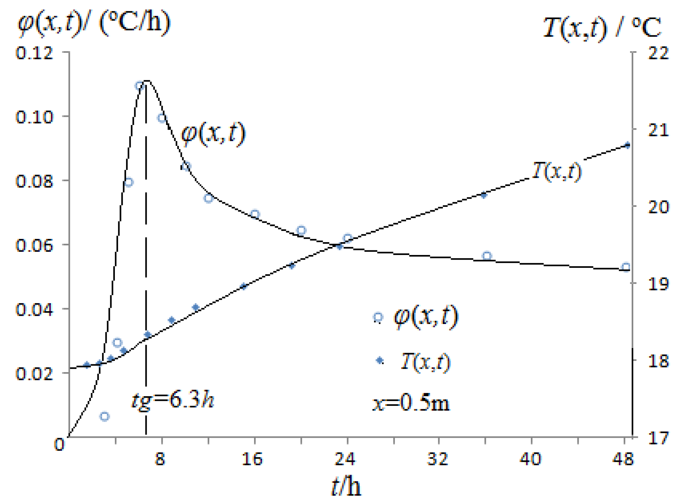
In a continuous 2D experiment, the initial temperature of the specimen was 18.06 °C. In the initial stage of the experiment, hot water at 36 °C was rapidly injected into the steel pipe, and then the water temperature was slowly decreased at an approximately constant rate using a resistance heater. At the end of the experiment, the water temperature reached 35.5 °C. Thus, in the experiment, ∆T0 was 17.94 °C and λ was −0.25 °C/d.
In the test, considering the influence of size, in the material with a length of 3.0 m, temperature measurements were recorded 0.5 m away from the heating device. The results are presented in Table 1. Note that the first two hours of the experiment have been excluded because the temperature readings in this period were not sensitive enough.
As shown in Figure 4, at the inflection point on the curve of φ(x, t) − t, tg = 6.3 h. According to Equation (28), the value of a is determined to be 1.85 × 10⁻⁶ m2/s. In the process of determining the inflection point from the measured temperature, this paper uses the forward-interpolation method based on the measured temperature to find the temperature change velocity φ(x, t), as listed in Table 1. According to the excerpting process of 1 h, the inflection point appears at around 6.3 h; if the calculation accuracy is not high enough, the encryption excerpt can be made near the inflection point. Additionally, using forward or backward interpolation to find the temperature change velocity φ(x, t) also has some influence on the determination of the inflection point time; however, this influence can be effectively avoided by employing multiple encryptions [36].

5.3.2. Calculation Example of Constant Temperature Boundary

In another continuous 2D test, the initial temperature of the specimen was 18.00 °C. At the initial stage of the test, hot water at 36 °C was rapidly injected into the steel pipe, and then the water temperature was kept approximately constant through the resistance heater until the end of the test when the water temperature reached 36.0 °C. The test data under this condition are presented in Table 2.
In the experiment, ∆T0 was 18 °C and λ was 0 °C/d.
Figure 5 shows that the actual measured T(x, t) point is located between the curve of a = 0.16 − 0.18 m2/d, and the value of a for the test material is approximately 0.17 m2/d, which is 1.98 × 10⁻⁶ m2/s.
The results obtained by the inflection point method and the wiring method are in general agreement with those of [22], which found a result of 1.94 × 10⁻⁶ m2/s.
In the case study, in the calculation using the inflection point method, when drawing the graph, determining the time tg at which the inflection point appears has a greater impact on the calculation of the a-value, and if the measurement time density interval of the temperature in the experiment is large, it may lead to a large error in the calculation of the a-value due to the inaccuracy of the determined tg. It is worth noting that in the existing literature, the φ(x, t) − t inflection point method is mostly used to find the a-value, and the curve fitting method is rarely studied. The curve fitting method, which can apply all the test data to the curve fitting process, requires the prior establishment of a theoretical curve family, and the workload is relatively large. Additionally, the influence of manual human judgment in the curve-fitting process is obvious; the self-applicable curve-fitting method can be adopted to avoid this influence effectively [36]. Alternatively, it is also possible to draw on some computational methods [37,38] or numerical algorithms [39] for building the solution to facilitate application.

5.3.3. Application in Engineering

For this work to have meaning, the solution must allow its application in engineering. The experimental method we proposed can be used to determine the thermal diffusivity. For example, in the design of a ground-source heat pump, due to the difficulty and high cost of testing the thermal physical parameters of the formation in the field, rock samples can be selected at the engineering site, and the steady-state method is used. Then the inflection point method and the curve fitting method are used to calculate thermal diffusivity or thermal conductivity of the actual drill core samples.
The steady-state method is to establish a stable temperature distribution inside the material, measure the temperature gradient and heat flux density inside the material, and then obtain the thermal conductivity of the measured material. The thermal diffusivity or thermal conductivity coefficient a is calculated according to the “steady-state method test”; generally, the boundary temperature f(t) needs to remain stable during the test. However, in the actual test process, it is difficult to keep f(t) unchanged due to the long test time of the “steady-state method”. The calculation method established in this paper can be effectively applied to the actual situation where f(t) has a certain range of slow change in the test.

6. Conclusions

The following conclusions were obtained in this paper by proposing a Laplace transform shortcut solution method for a one-dimensional heat conduction model with Dirichlet boundary conditions:
(1)
For the one-dimensional heat conduction model with the Dirichlet boundary function f(t), according to the differential properties of the Laplace transform and the convolution theorem, a general theoretical solution can be obtained as a product of erfc(t) and f(0), as well as erfc(t) and f(t). The general theoretical solution is derived for this type of model.
(2)
By substituting the boundary function f(t) into the general theoretical solution, the solution to practical problems can be obtained quickly. This shortcut solution method does not directly involve the transformation of f(t) and does not require a complex and cumbersome Laplace transform process.
(3)
With the temperature-based dynamic monitoring data and the time variation curve of the temperature change rate φ(x, t) − t, the model parameter “a” can be determined based on the fitting between the measured curve and the theoretical curve.
(4)
When calculating the temperature change rate φ(x, t) based on the measured temperature, using forward or backward interpolation has a certain influence on the results; when determining the time of the inflection point based on the self-recorded data, it is advisable to appropriately encrypt the data extraction time near the inflection point to avoid this influence.
Note that although the image function of f(t) with respect to the Laplace transform and the inverse function of the specific solution L[f(t)] exp ( s / a x ) are not directly obtained in the solving process, they are essentially involved in the Laplace transform process [40]. Therefore, f(t) must satisfy the basic requirements of the Laplace transform; it should be piecewise continuous on any interval for t ≥ 0 and have finite growth as t→∞ [3,41]. Most functions in engineering and technology satisfy this requirement.
In this paper, the Laplace transform shortcut solution to a one-dimensional heat transfer conduction model is presented. In engineering applications, the calculation of thermophysical parameters (i.e., thermal diffusivities or thermal conductivity coefficients in the model) of the test materials based on the methodology of this paper by using data from dynamic monitoring of the temperature field is one of the important purposes of the study of such problems. Thermal diffusivity is crucial to determine the dimension of the systems in civil engineering and initial investment. Considering the assumptions and the parameters that are used in deriving the analytical solution, and in order to use the analytical solution in this paper to determine all model parameters accurately, it is necessary to propose a more detailed field and indoor experimental approach to determine and measure all the physical parameters with precision. This is for further research.

Author Contributions

Conceptualization, D.W. and Y.T.; methodology, D.W.; validation, D.W.; formal analysis, D.W. and Y.T.; investigation, D.W.; resources, Y.T.; data curation, D.W.; writing—original draft preparation, D.W.; writing—review and editing, Y.T.; visualization, D.W.; supervision, Y.T.; project administration, H.R.; funding acquisition, H.R. All authors have read and agreed to the published version of the manuscript.

Funding

This research was funded by the National Natural Science Foundation of China (grant number 42107082, 42107162) and the National Key Research and Development Program of China (grant number 2018YFC1802700).

Institutional Review Board Statement

Not applicable.

Informed Consent Statement

Not applicable.

Data Availability Statement

Not applicable.

Acknowledgments

I would like to thank the editors, the referees and the editorial staff for all the help.

Conflicts of Interest

The authors declare no conflict of interest.

Nomenclature

athermal diffusivity, m2/s
fboundary temperature, °C
LLaplace transform operator
L−1inverse Laplace transform operator
u ¯ image function for Laplace transform
sLaplace operator
erfc(u)the complementary error function
δ(tti−1)Heaviside function
ttime, d
φtemperature variation rate of the calculation point, °C/h
λboundary temperature variation rate, °C/d
tgappearance of inflection point, h
Ttemperature of calculation point, °C
ΔT0instantaneous change in boundary temperature, °C
xdistance of the calculation point from the boundary, m
convolution operator

References

  1. Tao, W.Q. Heat Transfer Theory, 5th ed.; Higher Education Press: Beijing, China, 2019; pp. 75–77. [Google Scholar]
  2. Gu, C.H.; Li, D.Q.; Chen, S.X. Mathematical Physical Equation, 3rd ed.; Higher Education Press: Beijing, China, 2012; pp. 148–150. [Google Scholar]
  3. Zhang, Y.L. Integral Transformation, 4th ed.; Higher Education Press: Beijing, China, 2012; pp. 96–97. [Google Scholar]
  4. Hu, X.; Deng, S.; Wang, Y.; Chen, J.; Zhang, L.; Guo, W.; Han, Y. Study progress on analytical solution of static temperature field with artificial ground freezing. Mine Constr. Technol. 2015, 36, 1–9. [Google Scholar]
  5. Fabrea, A.; Hristov, J. On the integral-balance approach to the transient heat conduction with linearly temperature-dependent thermal diffusivity. Heat Mass Transf. 2016, 53, 177–204. [Google Scholar] [CrossRef]
  6. Falta, R.W.; Wang, W.W. A semi-analytical method for simulating matrix diffusion in numerical transport models. J. Contam. Hydrol. 2017, 197, 39–49. [Google Scholar] [CrossRef] [PubMed] [Green Version]
  7. Zhou, Q.; Oldenburg, C.M.; Rutqvist, J. Revisiting the analytical solutions of heat transport in fractured reservoirs using a generalized multirate memory function. Water Resour. Res. 2019, 55, 1405–1428. [Google Scholar] [CrossRef]
  8. BniLam, N.; Al-Khoury, R.; Shiri, A.; Sluys, L.J. A semi-analytical model for detailed 3D heat flow in shallow geothermal systems. Int. J. Heat Mass Transf. 2018, 123, 911–927. [Google Scholar] [CrossRef]
  9. Li, Y.; Shu, L.; Xiao, R.; Tao, Y.; Niu, S.; Wang, Z. Effect of pumping-recharge well structures on heat transfer characteristics of double-well groundwater heat pump systems considering hydrothermal coupling. Energy Convers. Manag. 2021, 249, 114871. [Google Scholar] [CrossRef]
  10. Povstenko, Y.; Klekot, J. Fractional heat conduction with heat absorption in a sphere under Dirichlet boundary condition. Comput. Appl. Math. 2018, 37, 4475–4483. [Google Scholar] [CrossRef] [Green Version]
  11. Hua, Y.C.; Zhao, T.; Guo, Z.Y. Optimization of the one-dimensional transient heat conduction problems using extended entransy analyses. Int. J. Heat Mass Transf. 2018, 116, 166–172. [Google Scholar] [CrossRef]
  12. Huang, D.; Li, Y.; Pei, D. Identification of a time-dependent coefficient in heat conduction problem by new iteration method. Adv. Math. Phys. 2018, 2018, 4918256. [Google Scholar] [CrossRef]
  13. Kot, V.A. Integral method of boundary characteristics: The Dirichlet condition. Principles. Heat Transf.Res. 2016, 47, 1035–1055. [Google Scholar] [CrossRef]
  14. Chen, H.L.; Liu, Z.L. Solving the inverse heat conduction problem based on data driven model. Chin. J. Comput. Mech. 2021, 38, 272–279. [Google Scholar]
  15. Sa, M.; Rw, Z. Laplace transform inversion for late-time behavior of groundwater flow problems. Water Resour. Res. 2003, 39, 1283. [Google Scholar]
  16. Sedghi, M.M.; Zhan, H. Groundwater dynamics due to general stream fluctuations in an unconfined single or dual-porosity aquifer subjected to general areal recharge. J. Hydrol. 2019, 574, 436–449. [Google Scholar] [CrossRef]
  17. Zhao, Y.; Zhang, Y.K.; Liang, X. Analytical solutions of three-dimensional groundwater flow to a well in a leaky sloping fault-zone aquifer. J. Hydrol. 2016, 539, 204–213. [Google Scholar] [CrossRef]
  18. Bansal, R.K. Groundwater flow in floping aquifer under localized transient recharge: Analytical study. J. Hydraul. Eng. 2013, 139, 1165–1174. [Google Scholar] [CrossRef]
  19. Saeedpanah, I.; Azar, R.G. Solution of unsteady flow in a confined aquifer interacting with a stream with exponentially decreasing stream stage. J. Hydrol. Eng. 2019, 24, 1–11. [Google Scholar] [CrossRef]
  20. Saeedpanah, I.; Azar, R.G. Modeling the river-aquifer via a new exact model under a more general function of river water level variation. Appl. Water Sci. 2023, 13, 95. [Google Scholar] [CrossRef]
  21. Wu, D.; Tao, Y.Z.; Lin, F. Application of unsteady phreatic flow model and its solution under the boundary control of complicated function. J. Hydraul. Eng. 2018, 49, 725–731. [Google Scholar]
  22. Wei, T.; Tao, Y.Z.; Ren, H.L.; Wu, D. The solution to one- dimensional heat conduction problem bounded by the exponential decay condition and its application. Chin. J. Appl. Mech. 2022, 39, 1135–1139,1202. [Google Scholar]
  23. Ren, H.L.; Tao, Y.Z.; Lin, F.; Wei, T. Analytical Solution to the One-Dimensional Unsteady Temperature Field near the Newtonian Cooling Boundary. Axioms 2023, 12, 61. [Google Scholar] [CrossRef]
  24. Zhang, J.P. Principles and methods of expressing segmented functions as a single equation using unit step functions. Teach. Res. 1994, 1, 24–26. [Google Scholar]
  25. Tang, Z.H.; Wang, R.Q. On Definitions and Natures of Dirac Function. J. Liuzhou Voc. Tech. Coll. 2009, 9, 76–78. [Google Scholar]
  26. Hu, C.J.; Wang, Y.Z. The Laplace transform problem related to series of functions. Eng. Math. 1991, 3, 165–717. [Google Scholar]
  27. Silva, S. Newton’s cooling law in generalised statistical mechanics. Phys. A Stat. Mech. Appl. 2021, 565, 125539. [Google Scholar] [CrossRef]
  28. Zhang, S.C. The available range of Newton’s law of cooling. Coll. Phys. 2000, 19, 36–37. [Google Scholar]
  29. Zhang, W.Z. Calculation of Unsteady Flow of Groundwater and Evaluation of Groundwater Resources; Science Press: Beijing, China, 1983; pp. 69–75. [Google Scholar]
  30. Alim, T.; Zhou, Z.F.; Mutalip, I. A universal solution to unstable groundwater movement in vicinity of canals. J. Hohai Univ. 2003, 31, 649–651. [Google Scholar]
  31. Yang, H.P.; Xie, X.Y.; Zhang, J.F. Analytical solution of one-dimensional transient phreatic flow and its application. Adv. Water Sci. 2004, 24, 82–86. [Google Scholar]
  32. Tang, Z.H.; Qian, G.H.; Qian, W.Q. Estimation of temperature-dependent function of thermal conductivity for a material. Chin. J. Comput. Mech. 2011, 28, 377–382. [Google Scholar]
  33. Li, Z.J.; Fu, X.; Shi, L.Q. Inversely identified natural ice thermal diffusivity by using measured vertical ice temperature profiles: Recent advancement and considerations. J. Glaciol. Geocryolo. 2023, 45, 599–611. [Google Scholar]
  34. Dominic, G. Analytical solution to the unsteady one-dimensional conduction problem with two time-varying boundary conditions: Duhamel’s theorem and separation of variables. Heat Mass Transf. 2010, 46, 707–716. [Google Scholar]
  35. Tadue, A.; Chen, C.S.; Antonio, J. A boundary meshless method for solving heat transfer problems using the Fourier transform. Adv. Appl. Math. Mech. 2011, 3, 572–585. [Google Scholar] [CrossRef]
  36. He, L.X.; Li, B.J.; Long, Y.; Zhang, Z. Intelligent Optimization Curve Fitting of the Newman Model for the Unsteady Flow of Submerged Aquifer. Haihe Water Resour. 2023, 5, 60–65. [Google Scholar]
  37. Akbıyık, M.; Yamaç Akbıyık, S.; Karaca, E.; Yılmaz, F. De Moivre’s and Euler Formulas for Matrices of Hybrid Numbers. Axioms 2021, 10, 213. [Google Scholar] [CrossRef]
  38. Nichita, F.F. Unifification Theories: Rings, Boolean Algebras and Yang–Baxter Systems. Axioms 2023, 12, 341. [Google Scholar] [CrossRef]
  39. Batiha, I.M.; Abubaker, A.A.; Jebril, I.H.; Al-Shaikh, S.B.; Matarneh, K. A Numerical Approach of Handling Fractional Stochastic Differential Equations. Axioms 2023, 12, 388. [Google Scholar] [CrossRef]
  40. Ma, S.H. Laplace transformation the uniqueness of primitive function and inverse image function. J. Xi’an Aero. Tech. Coll. 2002, 2, 47–48. [Google Scholar]
  41. Teng, Y.M. Some problems in integeral transform. Coll. Math. 2015, 31, 105–109. [Google Scholar]
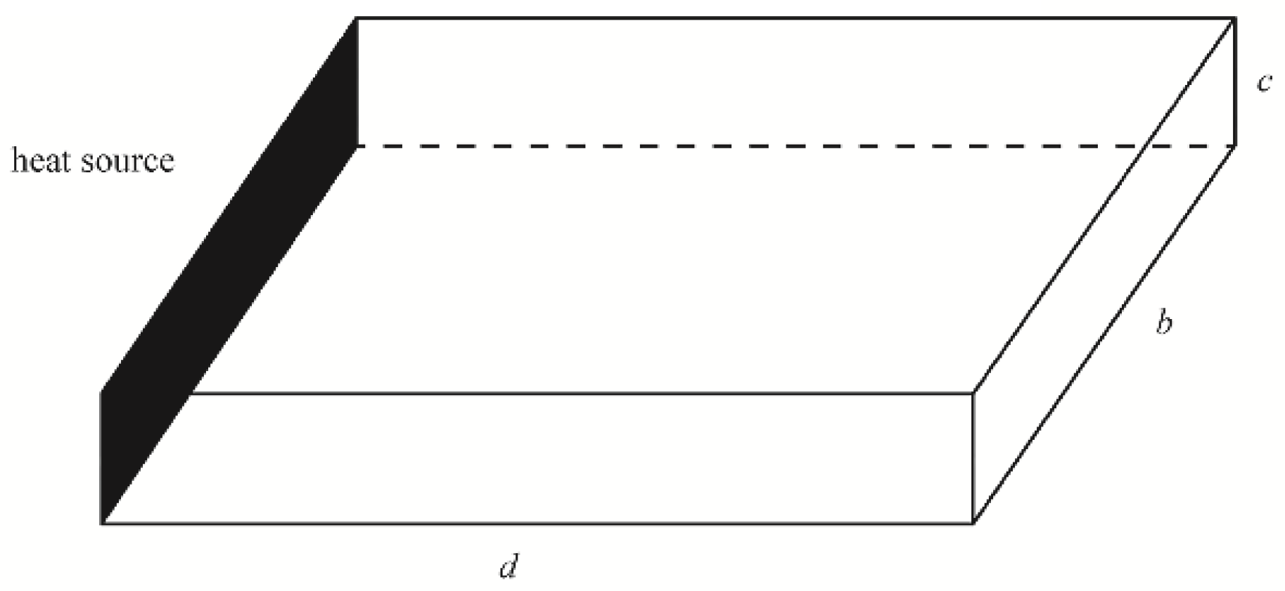
Figure 1. Schematic diagram corresponding to the physical model.
Axioms 12 00770 g001
Figure 2. The spatial variations in the temperature field near the boundaries.
Axioms 12 00770 g002
Figure 3. Discretization of boundary function f(t).
Axioms 12 00770 g003
Figure 4. The inflection point method for finding a.
Axioms 12 00770 g004
Figure 5. T(x,t) − t curve fitting method for a.
Axioms 12 00770 g005
Table 1. Temperature measurements at x = 0.5 m with variable temperature boundary.
t/h3456810121620243648
T(x,t)/°C17.9617.9718.0318.1418.3518.5318.718.9819.2419.4920.1720.81
φ(x,t)/(°C/h)0.007 0.010 0.060 0.110 0.105 0.090 0.085 0.070 0.065 0.063 0.057 0.053
Table 2. Temperature measurements at x = 0.5 m with constant temperature boundary.
t/h2346810121620243648
T(x,t)/°C22.123.8525.0926.8327.9428.6929.2330.1630.7531.163232.58
Disclaimer/Publisher’s Note: The statements, opinions and data contained in all publications are solely those of the individual author(s) and contributor(s) and not of MDPI and/or the editor(s). MDPI and/or the editor(s) disclaim responsibility for any injury to people or property resulting from any ideas, methods, instructions or products referred to in the content.