Handling a Commensurate, Incommensurate, and Singular Fractional-Order Linear Time-Invariant System

Abstract

From the perspective of the importance of the fractional-order linear time-invariant (FoLTI) system in plenty of applied science fields, such as control theory, signal processing, and communications, this work aims to provide certain generic solutions for commensurate and incommensurate cases of these systems in light of the Adomian decomposition method. Accordingly, we also generate another general solution of the singular FoLTI system with the use of the same methodology. Several more numerical examples are given to illustrate the core points of the perturbations of the considered singular FoLTI systems that can ultimately generate a variety of corresponding solutions.

1. Introduction

A fractional-order system is a dynamical system characterized by differential equations with noninteger-order derivatives. The integer-order representation is regarded as a specific instance of such systems, with fractional-order dynamics serving as the most generic description of the majority of realistic systems. Several kinds of fractional-order dynamical system challenges have recently been discussed in the literature [1,2,3,4,5].

In the late 1990s, the work on time-domain system identification using fractional-order models began. There are several techniques to discretize fractional-order differential equations by utilizing the phase assignment approach or the Grunwald–Letnikov approximation, which can be found in [6]. Moreover, the stability, observability, and controllability of fractional-order systems have been thoroughly examined using state-space representations (see [7,8,9]). In the same regard, there are several fields, including electric networks, economics, optimization issues, control system analysis, restricted mechanics, aircraft and robot dynamics, biology and large-scale systems, that depend heavily on the so-called singular fractional-order system of differential equations for their construction [10].

The Caputo fractional-order derivative operator has many applications in the field of applied science and engineering. For example, one application in applied mathematics for this operator is the study of natural convection flows of Prabhakar-like fractional Maxwell fluids with generalized thermal transport in the fractional case [11]. In general, this derivative can be defined as a combination of an integral of the function and a derivative of a lower order. The study of nonlocal transport phenomena, such as the generalized heat transport seen in some materials, makes use of this kind of derivative especially well. In particular, the Caputo fractional-order derivative operator and other equivalent fractional-order operators can offer precise and effective solutions to many intricate phenomena and systems (see [12,13]).

Using the ADM, nonlinear ordinary, partial, and fractional differential equations used in physics, mathematics, chemistry, and biology may be solved semianalytically. George Adomian, director of the University of Georgia’s Center for Applied Mathematics, created the technique between the 1970s and 1990s. The ADM decomposes a solution into an infinite series, which converges rapidly to the exact solution [14,15]. Basically, this technique was introduced to formulate approximate solutions for nonlinear systems. It is based on the decomposition of the nonlinear part of a differential system into a series of Adomian polynomials. The recursive formulation generated by the ADM corresponds to the technique proposed by Picard and Lindelöf to generate a solution to the initial value problem for a general expression of the differential system. Picard’s method is a basic technique that has been improved by ADM decomposition for the case of strongly nonlinear systems [16,17]. However, we think that these methods are equivalent in the case of dealing with linear systems. In this paper, with the use of the ADM, commensurate and incommensurate Fractional-order Linear Time-Invariant (FoLTI) systems are solved semianalytically. Accordingly, the singular FoLTI system is then solved by using the same methodology.

The remainder of this manuscript is constructed in the following manner. Section 2 aims to recollect some essential information and definitions regarding the Adomain decomposition method. Section 3 intends to illustrate the primary results of this work, including the results connected with the commensurate, incommensurate, and singular FoLTI systems. Section 4 aims to demonstrate several examples, followed by the last section, which outlines the concluding remarks of this work.

2. Adomain Decomposition Method

In this section, we recall the basic principles of the ADM concerning a nonlinear problem of the form

$$Lw+Rw+Nw=g,$$

(1)

where g is the system input, w is the system output, L is the linear operator that needs to be inverted, R is the linear remainder operator, and N is the nonlinear operator, which is assumed to be analytic. Herein, we emphasize that the choice for L and its inverse $L^{-1}$ are decided by the particular equation to be solved. Generally, we choose $L=\frac{d^m}{d{x}^m}(·)$ for the mth-order differential equations, and thus, its inverse $L^{-1}$ follows as the m-fold definite integration operator from $x_0$ to x. Consequently, we obtain $L^{-1}Lw=w-\psi$, where $\psi$ incorporates the initial values as $\psi ={\sum }_{v=0}^{m-1}{\beta }_v\frac{{(x-x_0)}^v}{v!}$. Now, applying the inverse linear operator $L^{-1}$ to both sides of (1) gives

$$w=\gamma \left(x\right)-L^{-1}[Rw+Nw],$$

(2)

where $\gamma \left(x\right)=\psi +L^{-1}g$. The ADM decomposes the solution into a series

$$w=\sum _{n=0}^{\infty }{w}_n,$$

(3)

and then decomposes the nonlinear term $Nw$ into a series

$$Nw=\sum _{n=0}^{\infty }{A}_n,$$

(4)

where $A_n$ are called the Adomian polynomials, which can be generated for the nonlinearity $Nw=f\left(w\right)$ by the following formula [18]:

$$A_n=\frac{1}{n!}\frac{{\partial }^n}{\partial {\lambda }^n}{\left[f\left(\sum _{k=0}^{\infty }{w}_k{\lambda }^k\right)\right]}_{\lambda =0},n=0,1,2,\cdots ,$$

(5)

where $\lambda$ is a grouping parameter of convenience.

For convenience, below, we list the formulas of the first Adomian polynomials for the one-variable nonlinearity $Nw=f\left(w\right(x\left)\right)$ from $A_0$ up to $A_5$:

$$\begin{array}{cc}\hfill A_0& =f\left(w_0\right),\hfill \\ \hfill A_1& =f^{\prime }\left(w_0\right)w_1,\hfill \\ \hfill A_2& =f^{\prime }\left(w_0\right)w_2+f^{\prime \prime }\left(w_0\right)\frac{w_1^2}{2!},\hfill \\ \hfill A_3& =f^{\prime }\left(w_0\right)w_3+f^{\prime \prime }\left(w_0\right)w_1{w}_2+f^{\left(3\right)}\left(w_0\right)\frac{w_1^3}{3!},\hfill \\ \hfill A_4& =f^{\prime }\left(w_0\right)w_4+f^{\prime \prime }\left(w_0\right)\left(\frac{w_2^2}{2!}+w_1{w}_3\right)+f^{\left(3\right)}\left(w_0\right)\frac{w_1^2{w}_2}{2!}+f^{\left(4\right)}\left(w_0\right)\frac{w_1^4}{4!},\hfill \\ \hfill A_5& =f^{\prime }\left(w_0\right)w_5+f^{\prime \prime }\left(w_0\right)(w_2{w}_3+w_1{w}_4)+f^{\left(3\right)}\left(w_0\right)\left(\frac{w_1{w}_2^2}{2!}+\frac{w_1^2{w}_3}{2!}\right)+f^{\left(4\right)}\left(w_0\right)\frac{w_1^3{w}_2}{3!}+f^{\left(5\right)}\left(w_0\right)\frac{w_1^5}{5!},\hfill \\ \hfill ⋮\end{array}$$

Accordingly, by substituting the Adomian decomposition series (3) for the solution $w\left(x\right)$ and the series of Adomian polynomials (4) suited to the nonlinearity $Nw$ into (2), we obtain

$$\sum _{n=0}^{\infty }{w}_n=\gamma \left(x\right)-L^{-1}\left[R\sum _{n=0}^{\infty }{w}_n+\sum _{n=0}^{\infty }{A}_n\right].$$

(6)

This consequently yields the following recursion states:

$$\begin{array}{cc}\hfill & w_0\left(x\right)=\gamma \left(x\right),\hfill \\ \hfill & w_{n+1}\left(x\right)=-L^{-1}[R{w}_n+A_n],n\ge 0,\hfill \end{array}$$

(7)

The n-term approximation of the solution is then of the form

$${\phi }_n\left(x\right)=\sum _{k=0}^{n-1}{w}_k\left(x\right).$$

(8)

It should be noted here that there are several alternative recursion approaches that can be used instead of (7), see, e.g., the Adomian–Rach [19], Wazwaz [20], Wazwaz-El-Sayed [21], Duan [22], and Duan–Rach [23].

3. FoLTI System

The state-space representation for the linear time-invariant system has the general form

$$\begin{array}{cc}\hfill {\mathbf{x}}^{\prime }\left(t\right)& =A\mathbf{x}\left(t\right)+B\mathbf{w}\left(t\right),\mathbf{x}\left(t_0\right)={\mathbf{x}}_0,\hfill \\ \hfill \mathbf{y}\left(t\right)& =C\mathbf{x}\left(t\right)+D\mathbf{w}\left(t\right),\hfill \end{array}$$

(9)

with the pseudo-state $\mathbf{x}\left(t\right)\in {\mathbb{R}}^n$, the input $\mathbf{w}\left(t\right)\in {\mathbb{R}}^p$, the output $\mathbf{y}\left(t\right)\in {\mathbb{R}}^q$, the order of differentiation $\alpha \in (0,1]$, and matrices of appropriate dimensions, namely the system matrix $A\in {\mathbb{R}}^{n\times n}$, the input matrix $B\in {\mathbb{R}}^{n\times p}$, the output matrix $C\in {\mathbb{R}}^{q\times n}$, and the feed through matrix $D\in {\mathbb{R}}^{q\times p}$ [24]. In particular, $\mathbf{x}\left(t\right)$ is the n-dimensional state vector, which can be expressed as

$$\mathbf{x}\left(t\right)=\left[\begin{array}{c}{x}_1\left(t\right)\\ x_2\left(t\right)\\ ⋮\\ x_n\left(t\right)\end{array}\right],$$

whose n scalar components are called state variables. Similarly, the m-dimensional input vector and p-dimensional output vector of $\mathbf{w}\left(t\right)$ and $\mathbf{y}\left(t\right)$ are given as

$$\mathbf{w}\left(t\right)=\left[\begin{array}{c}{w}_1\left(t\right)\\ w_2\left(t\right)\\ ⋮\\ w_m\left(t\right)\end{array}\right],\mathbf{y}\left(t\right)=\left[\begin{array}{c}{y}_1\left(t\right)\\ y_2\left(t\right)\\ ⋮\\ y_p\left(t\right)\end{array}\right].$$

In this connection, it should be mentioned that number three is a very critical issue concerning the use of the Caputo derivative and the concept of the state variable. In particular, the so-called initial condition of the Caputo derivative $x\left(0\right)$ is only related to instant $t_0$, whereas the dynamics of a fractional system refer to all the past behaviors of the system. Consequently, there is a need to correctly construct an approximate solution to the fractional system according to the initial conditions $x\left(0\right)$ by correctly considering the long memory feature of this system. In fact, this weak construction for such a solution may remain at any instant of $t>t_0$, and thus, $x\left(t\right)$ will not take into account the past behaviors of the system. This contradicts the definition of a state variable. In 2000, Lorenzo and Hartley addressed this matter by establishing a basic definition for initializing the fractional systems formulated by using the Riemann–Liouville and Grunwald fractional operators [25,26]. The Caputo fractional operator, which is used in this work, has not been considered regarding this issue until now. Actually, we believe that such an issue, which was inspired by the Lorenzo/Hartley approach and the infinite state representation, is regarded an important point and should be taken into account in the near future. However, in this work, we formulate and initialize the FoLTI system in light of the Caputo fractional derivative operator in its conventional form.

3.1. Commensurate FoLTI System

By replacing with the Caputo operator instead of using the classical one in the system (9), we can then generate the commensurate FoLTI system, which will be in the form

$$\left\{\begin{array}{cc}{D}_{*}^{\alpha }\mathbf{x}\left(t\right)=A\mathbf{x}\left(t\right)+B\mathbf{w}\left(t\right)& \\ \mathbf{y}\left(t\right)=C\mathbf{x}\left(t\right)+D\mathbf{w}\left(t\right).\end{array}\right.$$

(10)

subject to the initial condition

$$\mathbf{x}\left(t_0\right)={\mathbf{x}}_0.$$

(11)

Herein, $\alpha$ is the fractional-order value of the Caputo operator $D_{*}^{\alpha }$. This operator and its inverse (Riemann–Liouville fractional integrator) are recalled below for completeness.

Definition 1 

([27]). The Caputo fractional-order differential operator $D_{*}^{\alpha }$ of a function f is defined by

$$D_{*}^{\alpha }f\left(t\right)=\frac{1}{\mathrm{\Gamma }(m-\alpha )}{\int }_a^t\frac{f^{\left(m\right)}\left(u\right)}{{(t-u)}^{\alpha -m+1}}.du,$$

(12)

whenever the standard differential operator is $D^{m}f\in L_1[a,b]$, where $\alpha \ge 0$ and $m=\lceil \rho \rceil$.

Definition 2 

([27]). The Riemann–Liouville fractional-order integral operator $J_0^{\alpha }$ of a function $f\in L_1[a,b]$ is defined by

$$J_0^{\alpha }f\left(t\right)=\frac{1}{\mathrm{\Gamma }\left(\alpha \right)}{\int }_0^t{(t-u)}^{\alpha -1}f\left(u\right).du,$$

(13)

where $\alpha \in {\mathbb{R}}_{+}$ is the order of the operator, and $a\le t\le b$.

In this regard, we need to consider the following two important properties, that is, if $n-1<\alpha \le n$, where $n\in \mathbb{N}$, then [28]:

$$D_{*}^{\alpha }{J}_0^{\alpha }f\left(x\right)=f\left(x\right),$$

and

$$J_0^{\alpha }{D}_{*}^{\alpha }f\left(x\right)=f\left(x\right)-\sum _{i=1}^n{f}^i\left(0^{+}\right)\frac{x^i}{i!},x>0.$$

Now, in order to solve the first equations given in system (10) with the initial conditions (11) by using the ADM, we first add $J_0^{\alpha }$ to both sides of such equations to obtain

$$\mathbf{x}\left(t\right)=\mathbf{x}\left(0\right)+A{J}_0^{\alpha }\mathbf{x}\left(t\right)+B{J}_0^{\alpha }\mathbf{w}\left(t\right).$$

By considering the ADM, the general solution of the above equation can be assumed to be $\mathbf{x}\left(t\right)$=${\sum }_{n=0}^{\infty }{\mathbf{x}}_n\left(t\right)$. This consequently gives

$$\sum _{n=0}^{\infty }{\mathbf{x}}_n\left(t\right)={\mathbf{x}}_0+A{J}_0^{\alpha }\left(\sum _{n=0}^{\infty }{\mathbf{x}}_n\left(t\right)\right)+B{J}_0^{\alpha }\mathbf{w}\left(t\right),$$

which immediately implies

$$\begin{array}{cc}\hfill & x_0\left(t\right)={\mathbf{x}}_0+B{J}_0^{\alpha }\mathbf{w}\left(t\right)\hfill \\ \hfill & x_n\left(t\right)=A{J}_0^{\alpha }{\mathbf{x}}_{n-1}\left(t\right),n\ge 1.\hfill \end{array}$$

(14)

Thus, based on (14), we can obtain, for instance, ${\mathbf{x}}_1\left(t\right)$ as follows:

$${\mathbf{x}}_1\left(t\right)=\frac{A{\mathbf{x}}_0{t}^{\alpha }}{\mathrm{\Gamma }(\alpha +1)}+AB{J}_0^{2\alpha }\mathbf{w}\left(t\right).$$

In the same way, we can obtain

$${\mathbf{x}}_2\left(t\right)=\frac{A^2{\mathbf{x}}_0{t}^{2\alpha }}{\mathrm{\Gamma }(2\alpha +1)}+A^{2}B{J}_0^{3\alpha }\mathbf{w}\left(t\right).$$

If we continue in this manner, we can obtain

$${\mathbf{x}}_n\left(t\right)=\frac{A^n{\mathbf{x}}_0{t}^{n\alpha }}{\mathrm{\Gamma }(n\alpha +1)}+A^{n}B{J}_0^{(n+1)\alpha }\mathbf{w}\left(t\right),n\ge 1.$$

Now, due to the solution having the form $\mathbf{x}\left(t\right)={\sum }_{n=0}^{\infty }{\mathbf{x}}_n\left(t\right)$, then with the help of the Mittag–Leffler function, we can gain

$$\mathbf{x}\left(t\right)=E_{\alpha ,1}\left(A{t}^{\alpha }\right){\mathbf{x}}_0+{\int }_0^t{\left(t-\tau \right)}^{\alpha -1}{E}_{\alpha ,\alpha }\left(A{\left(t-\tau \right)}^{\alpha }\right)B\mathbf{w}\left(\tau \right)·d\tau ,$$

(15)

where $E_{·,·}\left(t\right)$ is the Mittag–Leffler function of two parameters, which is outlined by the next definition.

Definition 3 

([10]). The Mittag–Leffler function of two parameters α and β is outlined by the following series:

$$E_{\alpha ,\beta }\left(t\right)=\sum _{k=0}^{\infty }\frac{t^k}{\mathrm{\Gamma }(\alpha k+\beta )},$$

where $\alpha ,\beta >0$ and $t\in \mathbb{C}$.

In fact, solution (15) represents the solution of the first equations in system (10) according to the initial conditions (11). Hence, in order to find the solution of the output state $\mathbf{y}\left(t\right)$ reported in the second equation of system (10), we substitute (15) into this equation to obtain

$$\mathbf{y}\left(t\right)=C\left(E_{\alpha ,1}\left(A{t}^{\alpha }\right){\mathbf{x}}_0+{\int }_0^t{\left(t-\tau \right)}^{\alpha -1}{E}_{\alpha ,\alpha }\left(A{\left(t-\tau \right)}^{\alpha }\right)B\mathbf{w}\left(\tau \right)·d\tau \right)+D\mathbf{w}\left(t\right).$$

(16)

Hence, the two expressions reported in (15) and (16) represent the general solution to the FoLTI system.

3.2. Incommensurate FoLTI System

In this subsection, we deal with one of the most important systems, the incommensurate FoLTI system, which has the following form:

$$\left[\begin{array}{c}{D}^{\alpha }{\mathbf{x}}_1\left(t\right)\\ D^{\beta }{\mathbf{x}}_2\left(t\right)\end{array}\right]=\left[\begin{array}{cc}{A}_{11}& A_{12}\\ A_{21}& A_{22}\end{array}\right]\left[\begin{array}{c}{\mathbf{x}}_1\\ {\mathbf{x}}_2\end{array}\right]+\left[\begin{array}{c}{B}_1\\ B_2\end{array}\right]\mathbf{w}\left(t\right),$$

(17)

subject to the initial condition

$${\mathbf{x}}_0=\left[\begin{array}{c}{\mathbf{x}}_1\left(0\right)\\ {\mathbf{x}}_2\left(0\right)\end{array}\right],$$

where $0<\alpha ,\beta \le 1$, ${\mathbf{x}}_1\in {\mathbb{R}}^{n_1}$, ${\mathbf{x}}_2\in {\mathbb{R}}^{n_2}$, $\mathbf{w}\in {\mathbb{R}}^m$, $A_{ij}\in {\mathbb{R}}^{n_{i\times j}}$ and $B_i\in {\mathbb{R}}^{n_i}$, for $i,j=1,2$. In order to obtain the general solution to this system, we introduce the next result.

Lemma 1. 

System (17) has a solution of the form

$$\begin{array}{cc}\hfill \mathit{x}\left(t\right)=\sum _{k=0}^{\infty }\sum _{l=0}^{\infty }{\mathrm{\Phi }}_{kl}\frac{t^{k\alpha +\beta }{\mathit{x}}_0}{\mathrm{\Gamma }(k\alpha +l\beta +1)}& +{\int }_0^t\sum _{k=0}^{\infty }\sum _{l=0}^{\infty }{\mathrm{\Phi }}_{kl}\frac{{(t-\tau )}^{(k+1)\alpha +l\beta -1}}{\mathrm{\Gamma }\left(\right(k+1)\alpha +l\beta )}{B}_{10}\mathit{w}\left(\tau \right)·d\tau \hfill \\ \hfill & +{\int }_0^t\sum _{k=0}^{\infty }\sum _{l=0}^{\infty }{\mathrm{\Phi }}_{kl}\frac{{(t-\tau )}^{k\alpha +(l+1)\beta -1}}{\mathrm{\Gamma }(k\alpha +(l+1\left)\beta \right)}{B}_{01}\mathit{w}\left(\tau \right)·d\tau ,\hfill \end{array}$$

where

$$B_{10}=\left[\begin{array}{c}{B}_1\\ 0\end{array}\right],B_{01}=\left[\begin{array}{c}0\\ B_2\end{array}\right],$$

$${\mathrm{\Phi }}_{kl}=\left\{\begin{array}{cc}{I}_n& ,k=l=0\hfill \\ \left[\begin{array}{cc}{A}_{11}& A_{12}\\ 0& 0\end{array}\right]& ,k=1,l=0\hfill \\ \\ \left[\begin{array}{cc}0& 0\\ A_{21}& A_{22}\end{array}\right]& ,k=0,l=1\hfill \\ {\mathrm{\Phi }}_{10}{\mathrm{\Phi }}_{k-1,l}+{\mathrm{\Phi }}_{01}{\mathrm{\Phi }}_{k,l-1}& ,k+l>0.\hfill \end{array}\right.$$

Proof. 

To prove this result, we rewrite system (17) again in the form:

$$\begin{array}{cc}\hfill D^{\alpha }{\mathbf{x}}_1\left(t\right)& =A_{11}{\mathbf{x}}_1\left(t\right)+A_{12}{\mathbf{x}}_2\left(t\right)+B_1\mathbf{w}\left(t\right),\hfill \\ \hfill D^{\beta }{\mathbf{x}}_2\left(t\right)& =A_{21}{\mathbf{x}}_1\left(t\right)+A_{22}{\mathbf{x}}_2\left(t\right)+B_2\mathbf{w}\left(t\right).\hfill \end{array}$$

By adding $J_0^{\alpha }$ and $J_0^{\beta }$ to both sides of the above equations, we obtain

$$\begin{array}{cc}\hfill {\mathbf{x}}_1\left(t\right)& ={\mathbf{x}}_1\left(0\right)+A_{11}{J}_0^{\alpha }{\mathbf{x}}_1\left(t\right)+A_{12}{J}_0^{\alpha }{\mathbf{x}}_2\left(t\right)+B_1{J}_0^{\alpha }\mathbf{w}\left(t\right),\hfill \\ \hfill {\mathbf{x}}_2\left(t\right)& ={\mathbf{x}}_2\left(0\right)+A_{21}{J}_0^{\beta }{\mathbf{x}}_1\left(t\right)+A_{22}{J}_0^{\beta }{\mathbf{x}}_2\left(t\right)+B_2{J}_0^{\beta }\mathbf{w}\left(t\right).\hfill \end{array}$$

By considering the ADM, the general solution of the above equations can be assumed to be ${\mathbf{x}}_1\left(t\right)={\sum }_{n=0}^{\infty }{\mathbf{x}}_{1\left(n\right)}\left(t\right)$ and ${\mathbf{x}}_2\left(t\right)={\sum }_{n=0}^{\infty }{\mathbf{x}}_{2\left(n\right)}\left(t\right)$. This consequently gives

$$\begin{array}{cc}\hfill \sum _{n=0}^{\infty }{\mathbf{x}}_{1\left(n\right)}\left(t\right)& ={\mathbf{x}}_1\left(0\right)+A_{11}{J}_0^{\alpha }\left(\sum _{n=0}^{\infty }{\mathbf{x}}_{1\left(n\right)}\left(t\right)\right)+A_{12}{J}_0^{\alpha }\left(\sum _{n=0}^{\infty }{\mathbf{x}}_{2\left(n\right)}\left(t\right)\right)+B_1{J}_0^{\alpha }\mathbf{w}\left(t\right),\hfill \\ \hfill \sum _{n=0}^{\infty }{\mathbf{x}}_{2\left(n\right)}\left(t\right)& ={\mathbf{x}}_2\left(0\right)+A_{21}{J}_0^{\beta }\left(\sum _{n=0}^{\infty }{\mathbf{x}}_{1\left(n\right)}\left(t\right)\right)+A_{22}{J}_0^{\beta }\left(\sum _{n=0}^{\infty }{\mathbf{x}}_{2\left(n\right)}\left(t\right)\right)+B_2{J}_0^{\beta }\mathbf{w}\left(t\right),\hfill \end{array}$$

which implies

$$\begin{array}{cc}\hfill & {\mathbf{x}}_{1\left(0\right)}={\mathbf{x}}_1\left(0\right)+B_1{J}_0^{\alpha }\mathbf{w}\left(t\right), \hfill \end{array}$$

(18)

$$\begin{array}{cc}\hfill & {\mathbf{x}}_{1\left(n\right)}\left(t\right)=A_{11}{J}_0^{\alpha }{\mathbf{x}}_{1(n-1)}\left(t\right)+A_{12}{J}_0^{\alpha }{\mathbf{x}}_{2(n-1)}\left(t\right),n\ge 1,\hfill \end{array}$$

(19)

and

$$\begin{array}{cc}\hfill & {\mathbf{x}}_{2\left(0\right)}={\mathbf{x}}_2\left(0\right)+B_2{J}_0^{\beta }\mathbf{w}\left(t\right), \hfill \end{array}$$

(20)

$$\begin{array}{cc}\hfill & {\mathbf{x}}_{2\left(n\right)}\left(t\right)=A_{21}{J}_0^{\beta }{\mathbf{x}}_{1(n-1)}\left(t\right)+A_{22}{J}_0^{\beta }{\mathbf{x}}_{2(n-1)}\left(t\right),n\ge 1.\hfill \end{array}$$

(21)

Based on (18) and (19), we can obtain, for instance, ${\mathbf{x}}_{1\left(1\right)}\left(t\right)$, as follows:

$${\mathbf{x}}_{1\left(1\right)}\left(t\right)=\left(\frac{A_{11}{\mathbf{x}}_1\left(0\right)+A_{12}{\mathbf{x}}_2\left(0\right)}{\mathrm{\Gamma }(\alpha +1)}\right)t^{\alpha }+A_{11}{B}_1{J}_0^{2\alpha }\mathbf{w}\left(t\right)+A_{12}{B}_2{J}_0^{\alpha +\beta }\mathbf{w}\left(t\right).$$

In the same way, we can obtain

$${\mathbf{x}}_{2\left(1\right)}\left(t\right)=\left(\frac{A_{21}{\mathbf{x}}_1\left(0\right)+A_{22}{\mathbf{x}}_2\left(0\right)}{\mathrm{\Gamma }(\beta +1)}\right)t^{\beta }+A_{21}{B}_1{J}_0^{\alpha +\beta }\mathbf{w}\left(t\right)+A_{22}{B}_2{J}_0^{2\beta }\mathbf{w}\left(t\right).$$

In addition, we can obtain

$$\begin{array}{cc}\hfill {\mathbf{x}}_{1\left(2\right)}\left(t\right)=& \left(\frac{A_{11}^2{\mathbf{x}}_1\left(0\right)+A_{11}{A}_{12}{\mathbf{x}}_2\left(0\right)}{\mathrm{\Gamma }(2\alpha +1)}\right)t^{2\alpha }+A_{11}^2{B}_1{J}_0^{3\alpha }\mathbf{w}\left(t\right)+\left(A_{11}{A}_{12}{B}_2+A_{12}{A}_{21}{B}_1\right)J_0^{2\alpha +\beta }\mathbf{w}\left(t\right)\hfill \\ & +\left(\frac{A_{12}{A}_{21}{\mathbf{x}}_1\left(0\right)+A_{12}{A}_{22}{\mathbf{x}}_2\left(0\right)}{\mathrm{\Gamma }(\alpha +\beta +1)}\right)t^{\alpha +\beta }+A_{12}{A}_{22}{B}_2{J}_0^{\alpha +2\beta }\mathbf{w}\left(t\right).\hfill \end{array}$$

On the other hand, we can similarly obtain

$${\mathbf{x}}_{2\left(2\right)}\left(t\right)=A_{21}{J}_0^{\beta }{\mathbf{x}}_{1\left(1\right)}\left(t\right)+A_{22}{J}_0^{\beta }{\mathbf{x}}_{2\left(1\right)}\left(t\right).$$

In other words, we have

$$\begin{array}{cc}\hfill {\mathbf{x}}_{2\left(2\right)}\left(t\right)=& \left(\frac{A_{21}{A}_{11}{\mathbf{x}}_1\left(0\right)+A_{21}{A}_{12}{\mathbf{x}}_2\left(0\right)}{\mathrm{\Gamma }(\alpha +\beta +1)}\right)t^{\alpha +\beta }+A_{21}{A}_{11}{B}_1{J}_0^{2\alpha +\beta }\mathbf{w}\left(t\right)\hfill \\ \hfill & +\left(A_{21}{A}_{12}{B}_2+A_{22}{A}_{21}{B}_1\right)J_0^{\alpha +2\beta }\mathbf{w}\left(t\right)+\left(\frac{A_{22}{A}_{21}{\mathbf{x}}_1\left(0\right)+A_{22}^2{\mathbf{x}}_2\left(0\right)}{\mathrm{\Gamma }(2\beta +1)}\right)t^{2\beta }+A_{22}^2{B}_2{J}_0^{3\beta }\mathbf{w}\left(t\right).\hfill \end{array}$$

In the same regard, we can obtain

$${\mathbf{x}}_{1\left(3\right)}\left(t\right)=A_{11}{J}_0^{\alpha }{\mathbf{x}}_{1\left(2\right)}\left(t\right)+A_{12}{J}_0^{\alpha }{\mathbf{x}}_{2\left(2\right)}\left(t\right),$$

which implies

$$\begin{array}{cc}\hfill {\mathbf{x}}_{1\left(3\right)}\left(t\right)=& \left(\frac{A_{11}^3{\mathbf{x}}_1\left(0\right)+A_{11}^2{A}_{12}{\mathbf{x}}_2\left(0\right)}{\mathrm{\Gamma }(3\alpha +1)}\right)t^{3\alpha }+A_{11}^3{B}_1{J}_0^{4\alpha }\mathbf{w}\left(t\right)\hfill \\ \hfill & +(A_{11}^2{A}_{12}{B}_2+A_{11}{A}_{12}{A}_{21}{B}_1+A_{12}{A}_{21}{A}_{11}{B}_1)J_0^{3\alpha +\beta }\mathbf{w}\left(t\right)\hfill \\ \hfill & +\left(\frac{A_{11}{A}_{12}{A}_{21}{\mathbf{x}}_1\left(0\right)+A_{11}{A}_{12}{A}_{22}{\mathbf{x}}_2\left(0\right)+A_{12}{A}_{21}{A}_{11}{\mathbf{x}}_1\left(0\right)+A_{12}{A}_{21}{A}_{12}{\mathbf{x}}_2\left(0\right)}{\mathrm{\Gamma }(2\alpha +\beta +1)}\right)t^{2\alpha +\beta }\hfill \\ \hfill & +\left(A_{11}{A}_{12}{A}_{22}{B}_2+A_{12}{A}_{21}{A}_{12}{B}_2+A_{12}{A}_{22}{A}_{21}{B}_1\right)J_0^{2\alpha +2\beta }\mathbf{w}\left(t\right)\hfill \\ \hfill & +\left(\frac{A_{12}{A}_{22}{A}_{21}{\mathbf{x}}_1\left(0\right)+A_{12}{A}_{22}^2{\mathbf{x}}_2\left(0\right)}{\mathrm{\Gamma }(\alpha +2\beta +1)}\right)t^{\alpha +2\beta }+A_{12}{A}_{22}^2{B}_2{J}_0^{\alpha +3\beta }\mathbf{w}\left(t\right).\hfill \end{array}$$

In the same regard, we can obtain

$${\mathbf{x}}_{2\left(3\right)}\left(t\right)=A_{21}{J}_0^{\beta }{\mathbf{x}}_{1\left(2\right)}\left(t\right)+A_{22}{J}_0^{\beta }{\mathbf{x}}_{2\left(2\right)}\left(t\right),$$

which gives

$$\begin{array}{cc}\hfill {\mathbf{x}}_{2\left(3\right)}=& \left(\frac{A_{21}{A}_{11}^2{\mathbf{x}}_1\left(0\right)+A_{21}{A}_{11}{A}_{12}{\mathbf{x}}_2\left(0\right)}{\mathrm{\Gamma }(2\alpha +\beta +1)}\right)t^{2\alpha +\beta }+A_{11}^2{A}_{21}{B}_1{J}_0^{3\alpha +\beta }\mathbf{w}\left(t\right)\hfill \\ \hfill & +\left(A_{21}{A}_{11}{A}_{12}{B}_2+A_{21}^2{A}_{12}{B}_1+A_{22}{A}_{21}{A}_{11}{B}_1\right)J_0^{2\alpha +2\beta }\mathbf{w}\left(t\right)\hfill \\ \hfill & +\left(\frac{A_{21}^2{A}_{12}{\mathbf{x}}_1\left(0\right)+A_{21}{A}_{12}{A}_{22}{\mathbf{x}}_2\left(0\right)+A_{22}{A}_{21}{A}_{11}{\mathbf{x}}_1\left(0\right)+A_{22}{A}_{21}{A}_{12}{\mathbf{x}}_2\left(0\right)}{\mathrm{\Gamma }(\alpha +2\beta +1)}\right)t^{\alpha +2\beta }\hfill \\ \hfill & +\left(A_{21}{A}_{12}{A}_{22}{B}_2+A_{22}{A}_{21}{A}_{12}{B}_2+A_{22}^2{A}_{21}{B}_1\right)J_0^{\alpha +3\beta }\mathbf{w}\left(t\right)\hfill \\ \hfill & +\left(\frac{A_{22}^2{A}_{21}{\mathbf{x}}_1\left(0\right)+A_{22}^3{\mathbf{x}}_2\left(0\right)}{\mathrm{\Gamma }(3\beta +1)}\right)t^{3\beta }+A_{22}^3{B}_2{J}_0^{4\beta }\mathbf{w}\left(t\right).\hfill \end{array}$$

Now, if we continue in this manner, we can have

$${\mathbf{x}}_1\left(t\right)=\sum _{n=0}^{\infty }{\mathbf{x}}_{1\left(n\right)}\left(t\right)={\mathbf{x}}_{1\left(0\right)}\left(t\right)+{\mathbf{x}}_{1\left(1\right)}\left(t\right)+{\mathbf{x}}_{1\left(2\right)}\left(t\right)+{\mathbf{x}}_{1\left(3\right)}\left(t\right)+\cdots ,$$

i.e.,

$$\begin{array}{cc}\hfill {\mathbf{x}}_1\left(t\right)=& \sum _{n=0}^{\infty }\frac{A_{11}^n{\mathbf{x}}_1\left(0\right)}{\mathrm{\Gamma }(n\alpha +1)}{t}^{n\alpha }+\sum _{n=0}^{\infty }\frac{A_{11}^n{A}_{12}{\mathbf{x}}_2\left(0\right)}{\mathrm{\Gamma }\left(\right(n+1)\alpha +1)}{t}^{(n+1)\alpha }+\sum _{n=0}^{\infty }{A}_{11}^n{B}_1{J}_0^{(n+1)\alpha }\mathbf{w}\left(t\right)\hfill \\ \hfill & +\sum _{n=0}^{\infty }\left(A_{12}\left(A_{11}^n{B}_2+n{A}_{11}^{n-1}{A}_{21}{B}_1\right)\right)J_0^{(n+1)\alpha +\beta }\mathbf{w}\left(t\right)\hfill \\ & +\sum _{n=0}^{\infty }{A}_{12}{A}_{22}^n\left(\frac{A_{21}{\mathbf{x}}_1\left(0\right)+A_{22}{\mathbf{x}}_2\left(0\right)}{\mathrm{\Gamma }(\alpha +(n+1)\beta +1)}\right)t^{\alpha +(n+1)\beta }\hfill \\ \hfill & +\sum _{n=1}^{\infty }\left(\frac{(n+1)A_{11}^n{A}_{12}{A}_{21}{\mathbf{x}}_1\left(0\right)+\left(A_{12}{A}_{22}{A}_{11}^n+n{A}_{12}^{n+1}{A}_{21}\right){\mathbf{x}}_2\left(0\right)}{\mathrm{\Gamma }\left(\right(n+1)\alpha +\beta +1)}\right)t^{(n+1)\alpha +\beta }\hfill \\ \hfill & +\sum _{n=1}^{\infty }\left(\left(A_{11}{A}_{12}{A}_{22}^n+n{A}_{12}^{n+1}{A}_{21}^n\right)B_2+A_{12}{A}_{21}{A}_{22}^n{B}_1\right)J_0^{2\alpha +(n+1)\beta }\mathbf{w}\left(t\right)\hfill \\ \hfill & +\sum _{n=0}^{\infty }{A}_{12}{A}_{22}^{n+1}{B}_2{J}_0^{\alpha +(n+2)\beta }\mathbf{w}\left(t\right)+\cdots .\hfill \end{array}$$

In a similar manner, we have

$${\mathbf{x}}_2\left(t\right)=\sum _{n=0}^{\infty }{\mathbf{x}}_{2\left(n\right)}\left(t\right)={\mathbf{x}}_{2\left(0\right)}\left(t\right)+{\mathbf{x}}_{2\left(1\right)}\left(t\right)+{\mathbf{x}}_{2\left(2\right)}\left(t\right)+{\mathbf{x}}_{2\left(3\right)}\left(t\right)+\cdots .$$

This means

$$\begin{array}{cc}\hfill {\mathbf{x}}_2\left(t\right)=& \sum _{n=0}^{\infty }\frac{A_{22}^n{\mathbf{x}}_2\left(0\right)}{\mathrm{\Gamma }(n\beta +1)}{t}^{n\beta }+\sum _{n=0}^{\infty }\frac{A_{22}^n{A}_{21}{\mathbf{x}}_1\left(0\right)\beta }{\mathrm{\Gamma }\left(\right(n+1)\beta +1)}{t}^{(n+1)}+\sum _{n=0}^{\infty }{A}_{22}^n{B}_2{J}_0^{(n+1)\beta }\mathbf{w}\left(t\right)\hfill \\ \hfill & +\sum _{n=0}^{\infty }{A}_{11}^n{A}_{21}{B}_1{J}_0^{(n+1)\alpha +\beta }\mathbf{w}\left(t\right)+\sum _{n=0}^{\infty }\left(\frac{A_{21}{A}_{11}^{n+1}{\mathbf{x}}_1\left(0\right)+A_{21}{A}_{11}^n{A}_{12}{\mathbf{x}}_2\left(0\right)}{\mathrm{\Gamma }\left(\right(n+1)\alpha +\beta +1)}\right)t^{(n+1)\alpha +\beta }\hfill \\ \hfill & +\sum _{n=0}^{\infty }\left(A_{21}{A}_{12}{A}_{11}^n{B}_2+n{A}_{21}^{n+1}{A}_{12}{B}_1+A_{22}{A}_{21}{A}_{11}^n{B}_1\right)J_0^{(n+1)\alpha +2\beta }\mathbf{w}\left(t\right)\hfill \\ \hfill & +\sum _{n=1}^{\infty }\left(\frac{(n{A}_{21}^{n+1}{A}_{12}+A_{21}{A}_{11}{A}_{22}^n){\mathbf{x}}_1\left(0\right)+(n+1)A_{21}{A}_{12}{A}_{22}^n{\mathbf{x}}_2\left(0\right)}{\mathrm{\Gamma }(\alpha +(n+1)\beta +1)}\right)t^{\alpha +(n+1)\beta }\hfill \\ \hfill & +\sum _{n=2}^{\infty }\left(A_{22}^n{A}_{21}{B}_1+n{A}_{21}{A}_{12}{A}_{22}^{n-1}{B}_2\right)J_0^{\alpha +(n+1)\beta }\mathbf{w}\left(t\right)+\cdots .\hfill \end{array}$$

Now, by repeating this manner several times and by using the assumptions

$${\mathrm{\Phi }}_{kl}=\left\{\begin{array}{cc}{I}_n& ,k=l=0\hfill \\ \left[\begin{array}{cc}{A}_{11}& A_{12}\\ 0& 0\end{array}\right]& ,k=1,l=0\hfill \\ \\ \left[\begin{array}{cc}0& 0\\ A_{21}& A_{22}\end{array}\right]& ,k=0,l=1\hfill \\ {\mathrm{\Phi }}_{10}{\mathrm{\Phi }}_{k-1,l}+{\mathrm{\Phi }}_{01}{\mathrm{\Phi }}_{k,l-1}& ,k+l>0,\hfill \end{array}\right.$$

with

$$B_{10}=\left[\begin{array}{c}{B}_1\\ 0\end{array}\right],B_{01}=\left[\begin{array}{c}0\\ B_2\end{array}\right],$$

we reach the desired result, which completely coincides with the result found in [29]. □

3.3. Singular FoLTI System

Singular systems, which are also called descriptor systems, generalized systems, or differential/algebraic systems, are found in engineering systems, such as electrical and chemical processing circuits or power systems. In this section, we aim to consider the following singular FoLTI system:

$$\begin{array}{cc}\hfill E{D}_{*}^{\alpha }\mathbf{x}\left(t\right)& =A\mathbf{x}\left(t\right)+B\mathbf{w}\left(t\right),\mathbf{x}\left(0\right)={\mathbf{x}}_0,\hfill \\ \hfill \mathbf{y}\left(t\right)& =C\mathbf{x}\left(t\right)+D\mathbf{w}\left(t\right),\hfill \end{array}$$

(22)

where $\mathbf{x}\left(t\right)\in {\mathbb{R}}^n$, $\mathbf{w}\left(t\right)\in {\mathbb{R}}^m$, $\mathbf{y}\left(t\right)\in {\mathbb{R}}^p$, while $E,A\in {\mathbb{R}}^{n\times n}$, $B\in {\mathbb{R}}^{n\times m}$, $C\in {\mathbb{R}}^{p\times n}$ and $D\in {\mathbb{R}}^{p\times m}$. It should be mentioned here that E is a singular matrix. Thus, in order to deal with the first equation in system (22), we assume

$$E_n=\left(E-\frac{1}{n}I\right),n=1,2,3,\cdots .$$

(23)

This converts the singular matrix E into an approximate nonsingular matrix $E_n$, such that

$$\underset{n\to \infty }{lim}{E}_n=\underset{n\to \infty }{lim}\left(E-\frac{1}{n}I\right)=E.$$

Based on the above discussion, one may take the first equation of system (22) as follows

$$\left(E-\frac{1}{n}I\right)D_{*}^{\alpha }\mathbf{x}\left(t\right)=A\mathbf{x}\left(t\right)+B\mathbf{w}\left(t\right),\mathbf{x}\left(0\right)={\mathbf{x}}_0.$$

(24)

If one finds the solution to (24), then its limit as $n\to \infty$ is the solution to the first equation of system (22), provided that this solution must converge. However, to address this point clearly, we introduce the next result.

Lemma 2. 

The solution to system (24) has the form

$$\begin{array}{cc}\hfill {\mathit{x}}_n\left(t\right)=& E_{\alpha ,1}\left({\left(E-\frac{1}{n}I\right)}^{-1}A{t}^{\alpha }\right)\mathit{x}\left(0\right)\hfill \\ \hfill & +{\int }_0^t{\left(t-\tau \right)}^{\alpha -1}{E}_{\alpha ,\alpha }\left({\left(E-\frac{1}{n}I\right)}^{-1}A{\left(t-\tau \right)}^{\alpha }\right){\left(E-\frac{1}{n}I\right)}^{-1}B\mathit{w}\left(\tau \right)·d\tau ,\hfill \end{array}$$

(25)

for $n=1,2,3,\cdots$.

Proof. 

In order to prove this result, we first multiply (24) by ${\left(E-\frac{1}{n}I\right)}^{-1}$. This gives

$$D_{*}^{\alpha }\mathbf{x}\left(t\right)={\left(E-\frac{1}{n}I\right)}^{-1}A\mathbf{x}\left(t\right)+{\left(E-\frac{1}{n}I\right)}^{-1}B\mathbf{w}\left(t\right).$$

(26)

By adding $J_0^{\alpha }$ to both sides of (26), we obtain

$$\mathbf{x}\left(t\right)=\mathbf{x}\left(0\right)+{\left(E-\frac{1}{n}I\right)}^{-1}A{J}_0^{\alpha }\mathbf{x}\left(t\right)+{\left(E-\frac{1}{n}I\right)}^{-1}B{J}_0^{\alpha }\mathbf{w}\left(t\right).$$

Using ADM yields

$$\sum _{n=0}^{\infty }{\mathbf{x}}_n\left(t\right)=\mathbf{x}\left(0\right)+{\left(E-\frac{1}{n}I\right)}^{-1}A{J}_0^{\alpha }\sum _{n=0}^{\infty }{\mathbf{x}}_n\left(t\right)+{\left(E-\frac{1}{n}I\right)}^{-1}B{J}_0^{\alpha }\mathbf{w}\left(t\right).$$

This consequently implies

$$\begin{array}{cc}\hfill {\mathbf{x}}_0\left(t\right)& =\mathbf{x}\left(0\right)+{\left(E-\frac{1}{n}I\right)}^{-1}B{J}_0^{\alpha }\mathbf{w}\left(t\right),\hfill \\ \hfill {\mathbf{x}}_n\left(t\right)& ={\left(E-\frac{1}{n}I\right)}^{-1}A{J}_0^{\alpha }{\mathbf{x}}_{n-1}\left(t\right),n\ge 1.\hfill \end{array}$$

In view of the above relations, we can obtain

$${\mathbf{x}}_1\left(t\right)=\left(\frac{{\left(E-\frac{1}{n}I\right)}^{-1}A\mathbf{x}\left(0\right)}{\mathrm{\Gamma }(\alpha +1)}\right)t^{\alpha }+{\left(E-\frac{1}{n}I\right)}^{-1}A{\left(E-\frac{1}{n}I\right)}^{-1}B{J}_0^{2\alpha }\mathbf{w}\left(t\right).$$

Similarly, we can obtain ${\mathbf{x}}_2\left(t\right)$, as follows:

$${\mathbf{x}}_2\left(t\right)={\left(E-\frac{1}{n}I\right)}^{-1}A{J}_0^{\alpha }{\mathbf{x}}_1\left(t\right),$$

which implies

$${\mathbf{x}}_2\left(t\right)=\left(\frac{{\left({\left(E-\frac{1}{n}I\right)}^{-1}A\right)}^2\mathbf{x}\left(0\right)}{\mathrm{\Gamma }(2\alpha +1)}\right)t^{2\alpha }+{\left({\left(E-\frac{1}{n}I\right)}^{-1}A\right)}^2{\left(E-\frac{1}{n}I\right)}^{-1}B{J}_0^{3\alpha }\mathbf{w}\left(t\right).$$

In the same way, we can obtain ${\mathbf{x}}_3\left(t\right)$, as follows:

$${\mathbf{x}}_3\left(t\right)=\left(\frac{{\left({\left(E-\frac{1}{n}I\right)}^{-1}A\right)}^3\mathbf{x}\left(0\right)}{\mathrm{\Gamma }(3\alpha +1)}\right)t^{3\alpha }+{\left({\left(E-\frac{1}{n}I\right)}^{-1}A\right)}^3{\left(E-\frac{1}{n}I\right)}^{-1}B{J}_0^{4\alpha }\mathbf{w}\left(t\right).$$

If we continue in this manner, we obtain

$$\mathbf{x}\left(t\right)=\sum _{n=0}^{\infty }{\mathbf{x}}_n\left(t\right)={\mathbf{x}}_0\left(t\right)+{\mathbf{x}}_1\left(t\right)+{\mathbf{x}}_2\left(t\right)+{\mathbf{x}}_3\left(t\right)+\cdots .$$

This means

$$\begin{array}{cc}\hfill \mathbf{x}\left(t\right)=\mathbf{x}\left(0\right)& +{\left(E-\frac{1}{n}I\right)}^{-1}B{J}_0^{\alpha }\mathbf{w}\left(t\right)+\left(\frac{{\left(E-\frac{1}{n}I\right)}^{-1}A\mathbf{x}\left(0\right)}{\mathrm{\Gamma }(\alpha +1)}\right)t^{\alpha }\hfill \\ \hfill & +{\left(E-\frac{1}{n}I\right)}^{-1}A{\left(E-\frac{1}{n}I\right)}^{-1}B{J}_0^{2\alpha }\mathbf{w}\left(t\right)+\left(\frac{{\left({\left(E-\frac{1}{n}I\right)}^{-1}A\right)}^2\mathbf{x}\left(0\right)}{\mathrm{\Gamma }(2\alpha +1)}\right)t^{2\alpha }\hfill \\ \hfill & +{\left({\left(E-\frac{1}{n}I\right)}^{-1}A\right)}^2{\left(E-\frac{1}{n}I\right)}^{-1}B{J}_0^{3\alpha }\mathbf{w}\left(t\right)+\left(\frac{{\left({\left(E-\frac{1}{n}I\right)}^{-1}A\right)}^3\mathbf{x}\left(0\right)}{\mathrm{\Gamma }(3\alpha +1)}\right)t^{3\alpha }\hfill \\ \hfill & +{\left({\left(E-\frac{1}{n}I\right)}^{-1}A\right)}^3{\left(E-\frac{1}{n}I\right)}^{-1}B{J}_0^{4\alpha }\mathbf{w}\left(t\right)+\cdots .\hfill \end{array}$$

Thus, we can obtain the general solution to (24), which is in the form

$$\begin{array}{cc}\hfill {\mathbf{x}}_n\left(t\right)=& E_{\alpha ,1}\left({\left(E-\frac{1}{n}I\right)}^{-1}A{t}^{\alpha }\right)\mathbf{x}\left(0\right)\hfill \\ \hfill & +\sum _{n=0}^{\infty }\frac{{\left({\left(E-\frac{1}{n}I\right)}^{-1}A\right)}^n{\left(E-\frac{1}{n}I\right)}^{-1}B}{\mathrm{\Gamma }\left(\left(n+1\right)\alpha \right)}{\int }_0^t{\left(t-\tau \right)}^{(n+1)\alpha -1}\mathbf{w}\left(\tau \right)·d\tau .\hfill \end{array}$$

This leads to the following assertion:

$$\begin{array}{cc}\hfill {\mathbf{x}}_n\left(t\right)=& E_{\alpha ,1}\left({\left(E-\frac{1}{n}I\right)}^{-1}A{t}^{\alpha }\right)\mathbf{x}\left(0\right)\hfill \\ \hfill & +{\int }_0^t{\left(t-\tau \right)}^{\alpha -1}\sum _{n=0}^{\infty }\frac{{\left({\left(E-\frac{1}{n}I\right)}^{-1}A{\left(t-\tau \right)}^{\alpha }\right)}^n}{\mathrm{\Gamma }(n\alpha +\alpha )}{\left(E-\frac{1}{n}I\right)}^{-1}B\mathbf{w}\left(\tau \right)·d\tau ,\hfill \end{array}$$

which gives the desired result that represents the general form of system (24). □

Remark 1. 

One can observe that the solution to the system (22) is given by

$$\mathit{x}\left(t\right)=\underset{n\to \infty }{lim}{\mathit{x}}_n\left(t\right),$$

and then we can find $\mathit{y}\left(t\right)$ by using the second equation of the same system, where ${\mathit{x}}_n\left(t\right)$ was previously outlined in (25).

4. Illustrative Examples

The target of this section is to illustrate several numerical examples of the generated findings obtained in the previous section.

Example 1. 

Consider the commensurate FoLTI system (10) with

$$\begin{array}{cc}\hfill A& =\left[\begin{array}{cc}0& 1\\ 0& 0\end{array}\right],B=\left[\begin{array}{c}0\\ 1\end{array}\right],C=\left[\begin{array}{cc}1& 0\end{array}\right],D=0,\hfill \\ \hfill \mathit{w}\left(t\right)& =1\left(t\right)=\left\{\begin{array}{cc}1& ,t\ge 0\hfill \\ 0& ,t<0\hfill \end{array}\right.,{\mathit{x}}_0=\left[\begin{array}{c}1\\ 1\end{array}\right].\hfill \end{array}$$

Then, by using the solution to the system reported in (15), we can obtain

$$\mathit{x}\left(t\right)=E_{\alpha ,1}\left(A{t}^{\alpha }\right){\mathit{x}}_0+{\int }_0^t{\left(t-\tau \right)}^{\alpha -1}{E}_{\alpha ,\alpha }\left(A{\left(t-\tau \right)}^{\alpha }\right)B\mathit{w}\left(\tau \right)·d\tau .$$

(27)

In order to obtain the solution in its final form, we take the first term of solution (27), as follows:

$$E_{\alpha ,1}\left(A{t}^{\alpha }\right){\mathit{x}}_0=\sum _{k=0}^{\infty }\frac{A^k{t}^{\alpha k}}{\mathrm{\Gamma }(\alpha k+1)}{\mathit{x}}_0=\left(I+\frac{A{t}^{\alpha }}{\mathrm{\Gamma }(\alpha +1)}+\frac{A^2{t}^{2\alpha }}{\mathrm{\Gamma }(2\alpha +1)}+\frac{A^3{t}^{3\alpha }}{\mathrm{\Gamma }(3\alpha +1)}+\cdots \right)\left[\begin{array}{c}1\\ 1\end{array}\right].$$

However, $A^k=0$ for $k=2,3,4,\cdots$. Then, we have

$$E_{\alpha ,1}\left(A{t}^{\alpha }\right){\mathit{x}}_0=\left[\begin{array}{c}1+\frac{t^{\alpha }}{\mathrm{\Gamma }(\alpha +1)}\\ 1\end{array}\right].$$

(28)

Now, we need to deal with the second term of solution (27). For this purpose, we take

$$E_{\alpha ,\alpha }\left(A{t}^{\alpha }\right)=\sum _{k=0}^{\infty }\frac{A^k{t}^{\alpha k}}{\mathrm{\Gamma }(\alpha k+\alpha )}=\frac{I}{\mathrm{\Gamma }\left(\alpha \right)}+\frac{A{t}^{\alpha }}{\mathrm{\Gamma }\left(2\alpha \right)}+\frac{A^2{t}^{2\alpha }}{\mathrm{\Gamma }\left(3\alpha \right)}+\cdots .$$

Again, due to $A^k=0$ for $k=2,3,4,\cdots$, we have

$${\int }_0^t{\left(t-\tau \right)}^{\alpha -1}{E}_{\alpha ,\alpha }\left(A{\left(t-\tau \right)}^{\alpha }\right)B\mathit{w}\left(\tau \right)·d\tau =\left[\begin{array}{c}\frac{t^{2\alpha }}{\mathrm{\Gamma }(2\alpha +1)}\\ \frac{t^{\alpha }}{\mathrm{\Gamma }(\alpha +1)}\end{array}\right].$$

(29)

By substituting (28) and (29) into (27), we obtain

$$\mathit{x}\left(t\right)=\left[\begin{array}{c}1+\frac{t^{\alpha }}{\mathrm{\Gamma }(\alpha +1)}+\frac{t^{2\alpha }}{\mathrm{\Gamma }(2\alpha +1)}\\ 1+\frac{t^{\alpha }}{\mathrm{\Gamma }(\alpha +1)}\end{array}\right],$$

(30)

which represents the final form of the solution to the first equation related to the commensurate FoLTI system under consideration. To obtain the solution to the second equation, one may easily substitute (30) into the equation, as follows:

$$\mathit{y}\left(t\right)=1+\frac{t^{\alpha }}{\mathrm{\Gamma }(\alpha +1)}+\frac{t^{2\alpha }}{\mathrm{\Gamma }(2\alpha +1)}.$$

(31)

Thus, the solution to the commensurate FoLTI system is expressed by (30) and (31).

Example 2. 

Consider the first equation of system (22) with

$$E=\left[\begin{array}{cc}0& 1\\ 0& 0\end{array}\right],A=I_2,B=\left[\begin{array}{c}1\\ 0\end{array}\right],\mathit{w}\left(t\right)=1\left(t\right)and{\mathit{x}}_0=\left[\begin{array}{c}1\\ 1\end{array}\right],$$

i.e., we have

$$\left[\begin{array}{cc}0& 1\\ 0& 0\end{array}\right]\left[\begin{array}{c}{D}_{*}^{\alpha }{\mathit{x}}_1\left(t\right)\\ D_{*}^{\alpha }{\mathit{x}}_2\left(t\right)\end{array}\right]=\left[\begin{array}{c}{\mathit{x}}_1\left(t\right)\\ {\mathit{x}}_2\left(t\right)\end{array}\right]+\left[\begin{array}{c}1\\ 0\end{array}\right].$$

(32)

Herein, we take

$$E_n=\left(E-\frac{1}{n}I\right),n=1,2,3,\cdots ,$$

(33)

and hence system (32) is

$$\left[\begin{array}{cc}-\frac{1}{n}& 1\\ 0& -\frac{1}{n}\end{array}\right]\left[\begin{array}{c}{D}_{*}^{\alpha }{\mathit{x}}_1\left(t\right)\\ D_{*}^{\alpha }{\mathit{x}}_2\left(t\right)\end{array}\right]=\left[\begin{array}{c}{\mathit{x}}_1\left(t\right)\\ {\mathit{x}}_2\left(t\right)\end{array}\right]+\left[\begin{array}{c}1\\ 0\end{array}\right].$$

With the help of the general solution (25), we can obtain

$$\begin{array}{cc}\hfill {\mathit{x}}_n\left(t\right)=& E_{\alpha ,1}\left({\left[\begin{array}{cc}-\frac{1}{n}& 1\\ 0& -\frac{1}{n}\end{array}\right]}^{-1}{t}^{\alpha }\right)\left[\begin{array}{c}1\\ 1\end{array}\right]\hfill \\ & +{\int }_0^t{\left(t-\tau \right)}^{\alpha -1}{E}_{\alpha ,\alpha }\left({\left[\begin{array}{cc}-\frac{1}{n}& 1\\ 0& -\frac{1}{n}\end{array}\right]}^{-1}{\left(t-\tau \right)}^{\alpha }\right){\left[\begin{array}{cc}-\frac{1}{n}& 1\\ 0& -\frac{1}{n}\end{array}\right]}^{-1}\left[\begin{array}{c}1\\ 0\end{array}\right]1\left(\tau \right)·d\tau ,\hfill \end{array}$$

for $n=1,2,3,\cdots$. Consequently, we have

$$\begin{array}{cc}\hfill {\mathit{x}}_n\left(t\right)=& \sum _{k=0}^{\infty }\frac{{\left(\left[\begin{array}{cc}-n& -n^2\\ 0& -n\end{array}\right]t^{\alpha }\right)}^k}{\mathrm{\Gamma }(\alpha k+1)}\left[\begin{array}{c}1\\ 1\end{array}\right]\hfill \\ & +{\int }_0^t{\left(t-\tau \right)}^{\alpha -1}\sum _{k=0}^{\infty }\frac{{\left(\left[\begin{array}{cc}-n& -n^2\\ 0& -n\end{array}\right]{\left(t-\tau \right)}^{\alpha }\right)}^k}{\mathrm{\Gamma }(\alpha k+\alpha )}\left[\begin{array}{cc}-n& -n^2\\ 0& -n\end{array}\right]\left[\begin{array}{c}1\\ 0\end{array}\right]·d\tau .\hfill \end{array}$$

This means

$$\begin{array}{cc}\hfill {\mathit{x}}_n\left(t\right)& =\left[\begin{array}{c}\sum _{k=0}^{\infty }\frac{{\left(-n{t}^{\alpha }\right)}^k}{\mathrm{\Gamma }(\alpha k+1)}+n\sum _{k=0}^{\infty }k\frac{{\left(-n{t}^{\alpha }\right)}^k}{\mathrm{\Gamma }(\alpha k+1)}\\ \sum _{k=0}^{\infty }\frac{{\left(-n{t}^{\alpha }\right)}^k}{\mathrm{\Gamma }(\alpha k+1)}\end{array}\right]+{\int }_0^t\sum _{k=0}^{\infty }\frac{{\left(-n\right)}^k{\left(t-\tau \right)}^{\alpha k+\alpha -1}}{\mathrm{\Gamma }(\alpha k+\alpha )}\left[\begin{array}{c}-n\\ 0\end{array}\right]·d\tau .\hfill \end{array}$$

This implies

$$\begin{array}{c}\hfill {\mathit{x}}_n\left(t\right)=\left[\begin{array}{c}{E}_{\alpha ,1}\left(-n{t}^{\alpha }\right)+nk{E}_{\alpha ,1}\left(-n{t}^{\alpha }\right)-n{t}^{\alpha }{E}_{\alpha ,\alpha +1}\left(-n{t}^{\alpha }\right)\\ E_{\alpha ,1}\left(-n{t}^{\alpha }\right)\end{array}\right],n=1,2,3,\cdots .\end{array}$$

In order to see how ${\mathbf{x}}_1\left(t\right)$ and ${\mathbf{x}}_2\left(t\right)$ appear, we plot Figure 1, Figure 2, Figure 3 and Figure 4 for $n=1,2,3,4,5$. In particular, Figure 1 and Figure 2 illustrate, respectively, the solution ${\mathbf{x}}_1\left(t\right)$ according to $\alpha =0.75$ and $\alpha =1$ for $n=1,2,3,4,5$. On the other hand, Figure 3 and Figure 4 show, respectively, the solution ${\mathbf{x}}_2\left(t\right)$ according to $\alpha =0.75$ and $\alpha =1$ for $n=1,2,3,4,5$.

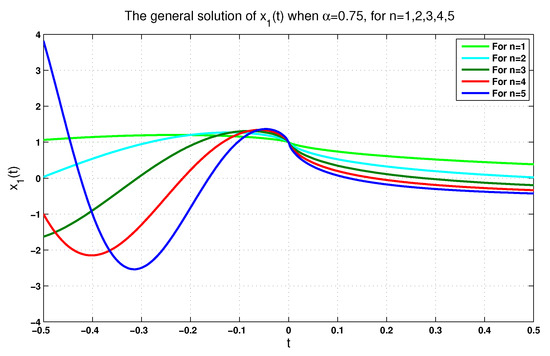
Figure 1. The solution ${\mathbf{x}}_1\left(t\right)$ when $\alpha =0.75$ for $n=1,2,3,4,5$.

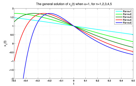
Figure 2. The solution ${\mathbf{x}}_1\left(t\right)$ when $\alpha =1$ for $n=1,2,3,4,5$.

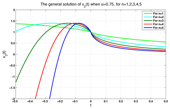
Figure 3. The solution ${\mathbf{x}}_2\left(t\right)$ when $\alpha =0.75$ for $n=1,2,3,4,5$.

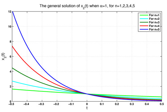
Figure 4. The solution ${\mathbf{x}}_2\left(t\right)$ when $\alpha =1$ for $n=1,2,3,4,5$.

Example 3. 

Consider a singular FoLTI system (22) with

$$\begin{array}{cc}\hfill & E=\left[\begin{array}{cccc}1& 0& 0& 0\\ 0& 0& 1& 0\\ 0& 0& 0& 0\\ 0& 0& 0& 0\end{array}\right],A=\left[\begin{array}{cccc}0& 0& 0& 0\\ 1& 0& 0& 0\\ 0& 1& 0& 0\\ 0& 0& 0& 1\end{array}\right],B=0,\hfill \\ \hfill & C=\left[\begin{array}{cccc}1& 0& 1& 0\end{array}\right],D=0,\mathit{x}\left(0\right)=\left[\begin{array}{c}0\\ 1\\ 0\\ 0\end{array}\right].\hfill \end{array}$$

Observe that $det\left(E\right)=0$, and so, E is singular. This allows us to deal with the following system:

$$\left(E-\frac{1}{n}I\right)D_{*}^{\alpha }\mathit{x}\left(t\right)=A\mathit{x}\left(t\right),$$

with the initial condition

$$\mathit{x}\left(0\right)={\left[\begin{array}{cccc}0& 1& 0& 0\end{array}\right]}^T.$$

By using the general solution (25), we can obtain

$${\mathit{x}}_n\left(t\right)=\left[\begin{array}{cccc}0& 0& 0& 0\\ \frac{1}{n}\sum _{k=0}^{\infty }\frac{{\left(-n^2{t}^{\alpha }\right)}^k}{\mathrm{\Gamma }(\alpha k+1)}& \sum _{k=0}^{\infty }\frac{{\left(-n^2{t}^{\alpha }\right)}^k}{\mathrm{\Gamma }(\alpha k+1)}& 0& 0\\ \sum _{k=2}^{\infty }\frac{{\left(-1\right)}^k{n}^{2k-2}{t}^{\alpha k}}{\mathrm{\Gamma }(\alpha k+1)}& \frac{1}{n}\sum _{k=0}^{\infty }\frac{{\left(-n^2{t}^{\alpha }\right)}^k}{\mathrm{\Gamma }(\alpha k+1)}& 0& 0\\ 0& 0& 0& \sum _{k=0}^{\infty }\frac{{\left(-n{t}^{\alpha }\right)}^k}{\mathrm{\Gamma }(\alpha k+1)}\end{array}\right]\left[\begin{array}{c}0\\ 1\\ 0\\ 0\end{array}\right],n=1,2,3,\cdots .$$

This consequently implies

$${\mathit{x}}_n\left(t\right)=\left[\begin{array}{cccc}0& 0& 0& 0\\ \frac{1}{n}{E}_{\alpha ,1}\left(-n^2{t}^{\alpha }\right)& E_{\alpha ,1}\left(-n^2{t}^{\alpha }\right)& 0& 0\\ E_{\alpha ,1}\left(-n^2{t}^{\alpha }\right)-1& \frac{1}{n}{E}_{\alpha ,1}\left(-n^2{t}^{\alpha }\right)& 0& 0\\ 0& 0& 0& E_{\alpha ,1}\left(-n{t}^{\alpha }\right)\end{array}\right]\left[\begin{array}{c}0\\ 1\\ 0\\ 0\end{array}\right],n=1,2,3,\cdots ,$$

or

$${\mathit{x}}_n\left(t\right)=\left[\begin{array}{c}0\\ E_{\alpha ,1}\left(-n^2{t}^{\alpha }\right)\\ \frac{1}{n}{E}_{\alpha ,1}\left(-n^2{t}^{\alpha }\right)\\ 0\end{array}\right],n=1,2,3,\cdots .$$

(34)

Thus, we have

$${\mathit{y}}_n\left(t\right)=C{\mathit{x}}_n\left(t\right)=\left[\begin{array}{cccc}1& 0& 1& 0\end{array}\right]\left[\begin{array}{c}0\\ E_{\alpha ,1}\left(-n^2{t}^{\alpha }\right)\\ \frac{1}{n}{E}_{\alpha ,1}\left(-n^2{t}^{\alpha }\right)\\ 0\end{array}\right],n=1,2,3,\cdots .$$

(35)

This means

$${\mathit{y}}_n\left(t\right)=\frac{1}{n}{E}_{\alpha ,1}\left(-n^2{t}^{\alpha }\right),n=1,2,3,\cdots .$$

For further illustration and for $n=1,2,3,4,5$, we plot $x_2\left(t\right)$ reported in (34) in Figure 5 and Figure 6 according to $\alpha =0.75$ and $\alpha =1$, respectively. Similarly, we plot $x_3\left(t\right)$ reported in (34) in Figure 7 and Figure 8 according to $\alpha =0.75$ and $\alpha =1$. In addition to these plots and for the same values of n, we plot $y\left(t\right)$ given in Equation (35) in Figure 9 and Figure 10 according to the same values of $\alpha$$\left(\mathrm{i}.\mathrm{e}.,\alpha =0.75\mathrm{and}\alpha =1\right)$.

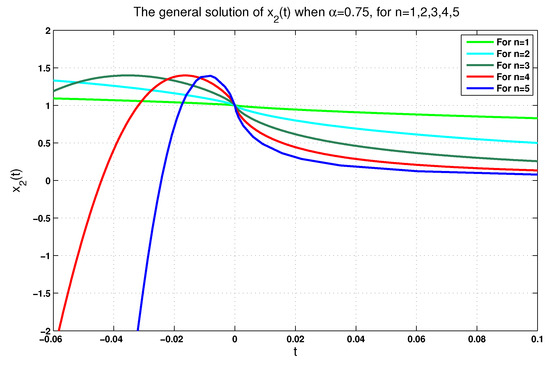
Figure 5. The general solution $x_2\left(t\right)$ when $\alpha =0.75$ for $n=1,2,3,4,5$.

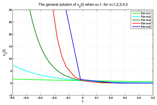
Figure 6. The general solution $x_2\left(t\right)$ when $\alpha =1$ for $n=1,2,3,4,5$.

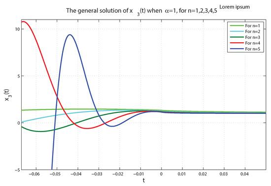
Figure 7. The general solution $x_3\left(t\right)$ when $\alpha =1$ for $n=1,2,3,4,5$.

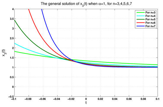
Figure 8. The general solution $x_3\left(t\right)$ when $\alpha =1$ for $n=3,4,5,6,7$.

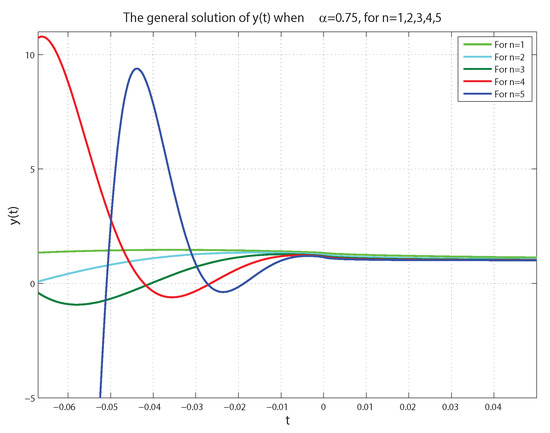
Figure 9. The general solution $y\left(t\right)$ when $\alpha =0.75$ for $n=1,2,3,4,5$.

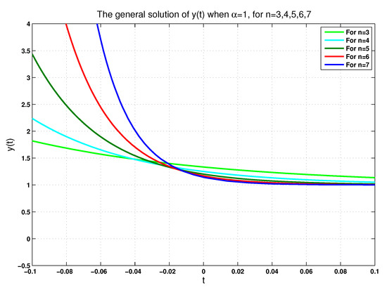
Figure 10. The general solution of $y\left(t\right)$ when $\alpha =1$ for $n=3,4,5,6,7$.

In fact, each figure of the previously performed simulations includes a single-phase trajectory of the phase variables $x_1$, $x_2$, $x_3$ and even y for $n=1,2,3,4,5$, once the value is $\alpha$ equal to 0.75, and again, when it is equal to 1. These (singular) perturbations of all singular FoLTI systems yield varying corresponding solutions. From a physical viewpoint, this is reasonable, since the physical system described by (22) is, in reality, probably described more precisely by (24). That is, (22) can be considered an idealized model of a higher-order system. We claim that the convergence of the solutions of (24) to zero on some subinterval of $(0,\infty )$ is, in fact, sufficient to guarantee that they also converge on a neighborhood of the origin. This claim is left for future consideration.

5. Conclusions

In this work, certain generic solutions for commensurate and incommensurate fractional-order linear time-invariant systems were successfully generated with the use of the Adomian decomposition method (ADM). As a result, a general solution of the singular fractional-order linear time-invariant system was obtained by using the same procedure. It was shown that the perturbations of all considered singular FoLTI systems yield varying corresponding solutions. For future consideration, we left the issue of proving that the singular FoLTI systems’ solutions converge to zero on some subinterval of $(0,\infty )$.

References

- Batiha, I.; Alshorm, S.; Jebril, I.; Hammad, M. A Brief Review about Fractional Calculus. Int. J. Open Probl. Comput. Sci. Math. 2022, 15, 39–56. [Google Scholar]
- Batiha, I.M.; Obeidat, A.; Alshorm, S.; Alotaibi, A.; Alsubaie, H.; Momani, S.; Albdareen, M.; Zouidi, F.; Eldin, S.M.; Jahanshah, H. A Numerical Confirmation of a Fractional-Order COVID-19 Model’s Efficiency. Symmetry 2022, 14, 2583. [Google Scholar] [CrossRef]
- Batiha, I.M.; Ababneh, O.Y.; Al-Nana, A.A.; Alshanti, W.G.; Alshorm, S.; Momani, S. A Numerical Implementation of Fractional-Order PID Controllers for Autonomous Vehicles. Axioms 2023, 12, 306. [Google Scholar] [CrossRef]
- Rania, S.; Qazza, A.; Burqan, A.; Al-Omari, S. On Time Fractional Partial Differential Equations and Their Solution by Certain Formable Transform Decomposition Method. Comput. Model. Eng. Sci. 2023, 136, 3121–3139. [Google Scholar]
- Bezziou, M.; Jebril, I.; Dahmani, Z. A new nonlinear duffing system with sequential fractional derivatives. Chaos Solitons Fractals 2021, 151, 111247. [Google Scholar] [CrossRef]
- Mathieu, B.; Lay, L.L.; Oustaloup, A. Identification of non integer order systems in the time domain. In Proceedings of the Symposium on Control, Optimization and Supervision, Lille, France, 9–12 July 1996; pp. 843–847. [Google Scholar]
- Ahmad, W.M.; El-Khazali, R.; Al-Assaf, Y. Stabilization of generalized fractional order chaotic systems using state feedback control. Chaos Solitons Fractals 2004, 22, 141–150. [Google Scholar] [CrossRef]
- Batiha, I.M.; Alshorm, S.; Ouannas, A.; Momani, S.; Ababneh, O.Y.; Albdareen, M. Modified Three-Point Fractional Formulas with Richardson Extrapolation. Mathematics 2022, 10, 3489. [Google Scholar] [CrossRef]
- Guechi, S.; Guechi, M. Taylor approximation for solving linear and nonlinear Ill-Posed Volterra equations via an iteration method. Gen. Lett. Math. 2022, 11, 18–25. [Google Scholar] [CrossRef]
- Podlubny, I. Fractional Differential Equations; Academic Press: San Diego, CA, USA, 1999. [Google Scholar]
- Shah, N.A.; Ebaid, A.; Oreyeni, T.; Yook, S.-J. MHD and porous effects on free convection flow of viscous fluid between vertical parallel plates: Advance thermal analysis. Waves Random Complex Media 2023, 1–13. [Google Scholar] [CrossRef]
- Shah, N.A.; Khan, I. Heat transfer analysis in a second grade fluid over and oscillating vertical plate using fractional Caputo–Fabrizio derivatives. Eur. Phys. J. C 2016, 75, 362. [Google Scholar] [CrossRef]
- Imran, M.A.; Khan, I.; Ahmad, M.; Shah, N.A.; Nazar, M. Heat and mass transport of differential type fluid with non-integer order time-fractional Caputo derivatives. J. Mol. Liq. 2017, 229, 67–75. [Google Scholar] [CrossRef]
- George, A. Solving Frontier Problems of Physics: The Decomposition Method; Springer Science & Business Media: Berlin/Heidelberg, Germany, 2013; Volume 60. [Google Scholar]
- George, A. Nonlinear Stochastic Operator Equations; Academic Press: Cambridge, MA, USA, 2014. [Google Scholar]
- Rach, R. On the Adomian (decomposition) method and comparisons with Picard’s method. J. Math. Anal. Appl. 1987, 128, 480–483. [Google Scholar] [CrossRef]
- El-Sayed, A.M.A.; Hashem, H.H.G.; Ziada, E.A.A. Picard and Adomian decomposition methods for a quadratic integral equation of fractional order. Comp. Appl. Math. 2014, 33, 95–109. [Google Scholar] [CrossRef]
- Adomian, G.; Rach, R. Inversion of nonlinear stochastic operators. J. Math. Anal. Appl. 1983, 91, 39–46. [Google Scholar] [CrossRef]
- Adomian, G.; Rach, R. Analytic solution of nonlinear boundary-value problems in several dimensions by decomposition. J. Math. Anal. Appl. 1993, 174, 118–137. [Google Scholar] [CrossRef]
- Abdul-Majid, W. A reliable modification of ADM. Appl. Math. Comput. 1999, 102, 77–86. [Google Scholar]
- Abdul-Majid, W.; El-Sayed, S.M. A new modification of the ADM for linear and nonlinear operators. Appl. Math. Comput. 2001, 122, 393–405. [Google Scholar]
- Duan, J.-S. Recurrence triangle for adomian polynomials. Appl. Math. Comput. 2010, 216, 1235–1241. [Google Scholar] [CrossRef]
- Duan, J.-S.; Rach, R. A new modification of the ADM for solving boundary value problems for higher order nonlinear differential equations. Appl. Math. Comput. 2011, 218, 4090–4118. [Google Scholar]
- Sabatier, J.; Farges, C.; Trigeassou, J.-C. Fractional systems state space description: Some wrong ideas and proposed solutions. J. Vib. Control 2014, 20, 1076–1084. [Google Scholar] [CrossRef]
- Lorenzo, C.F.; Hartley, T.T. Initialized fractional calculus. Int. J. Appl. Math. 2000, 3, 249–266. [Google Scholar]
- Maamri, N.; Trigeassou, J.-C. A Plea for the Integration of Fractional Differential Systems: The Initial Value Problem. Fractal Fract. 2022, 6, 550. [Google Scholar] [CrossRef]
- Diethelm, K. The Analysis of Fractional Differential Equations; Springer: Berlin/Heidelberg, Germany, 2004. [Google Scholar]
- Batiha, I.M.; Bataihah, A.; Al-Nana, A.A.; Alshorm, S.; Jebril, I.H.; Zraiqat, A. A numerical scheme for dealing with fractional initial value problem. Int. J. Innov. Comput. Inf. Control 2023, 19, 763–774. [Google Scholar]
- Kaczorek, T. Polynomial Approach to Fractional Descriptor Electrical Circuits; Computational Models for Business and Engineering Domains-ITHEA: Rzeszow, Poland, 2014. [Google Scholar]
Disclaimer/Publisher’s Note: The statements, opinions and data contained in all publications are solely those of the individual author(s) and contributor(s) and not of MDPI and/or the editor(s). MDPI and/or the editor(s) disclaim responsibility for any injury to people or property resulting from any ideas, methods, instructions or products referred to in the content. |
© 2023 by the authors. Licensee MDPI, Basel, Switzerland. This article is an open access article distributed under the terms and conditions of the Creative Commons Attribution (CC BY) license (https://creativecommons.org/licenses/by/4.0/).