Article

A Reliable Computational Scheme for Stochastic Reaction–Diffusion Nonlinear Chemical Model

by
Muhammad Shoaib Arif
1,2,*,
Kamaleldin Abodayeh
1 and
Yasir Nawaz
2
1
Department of Mathematics and Sciences, College of Humanities and Sciences, Prince Sultan University, Riyadh 11586, Saudi Arabia
2
Department of Mathematics, Air University, PAF Complex E-9, Islamabad 44000, Pakistan
*
Author to whom correspondence should be addressed.
Axioms 2023, 12(5), 460; https://doi.org/10.3390/axioms12050460
Submission received: 23 March 2023 / Revised: 30 April 2023 / Accepted: 5 May 2023 / Published: 9 May 2023
(This article belongs to the Special Issue Computational Mathematics in Engineering and Applied Science)

Abstract

:
The main aim of this contribution is to construct a numerical scheme for solving stochastic time-dependent partial differential equations (PDEs). This has the advantage of solving problems with positive solutions. The scheme provides conditions for obtaining positive solutions, which the existing Euler–Maruyama method cannot do. In addition, it is more accurate than the existing stochastic non-standard finite difference (NSFD) method. Theoretically, the suggested scheme is more accurate than the current NSFD method, and its stability and consistency analysis are also shown. The scheme is applied to the linear scalar stochastic time-dependent parabolic equation and the nonlinear auto-catalytic Brusselator model. The deficiency of the NSFD in terms of accuracy is also shown by providing different graphs. Many observable occurrences in the physical world can be traced back to certain chemical concentrations. Examining and understanding the inter-diffusion between chemical concentrations is important, especially when they coincide. The Brusselator model is the gold standard for describing the relationship between chemical concentrations and other variables in chemical systems. A computational code for the proposed model scheme may be made available to readers upon request for convenience.

1. Introduction

Since the beginning of life, humankind has faced natural calamities such as tsunamis, earthquakes, floods, drought, and pandemics. Diseases such as Ebola, HIV, Dengue virus, malaria, tuberculosis, influenza, diarrhea, hepatitis C, hepatitis B, and rubella strike without warning and have no set time or location. These diseases are not only confined to humans but also influence animals, which sometimes become the root cause of specific diseases. Therefore, economic recession, poor health conditions, and death toll have dramatically risen, resulting in uncertainty for the future generation.
The autocatalytic glycolysis model, the Gray–Scott reaction–diffusion system, and the Brusselator reaction–diffusion model are all examples of important reaction–diffusion models used to research biological and chemical processes. Prigogine was the first to propose the Brusselator reaction–diffusion model in 1970 [1], a model of an autocatalytic process that can predict oscillations in a chemical reaction. This reaction model solves several physical problems, such as the formation of the ozone layer from atomic oxygen through triple collision and enzymatic actions. It is a nonlinear model that precisely defines a physical system but cannot solve the problems of a physical system due to non-linearity. Solving the problems of physical systems possessing nonlinear behavior has been a matter of great concern for the past several decades. It is not simple to draw the solution; sometimes, it does not even exist. Therefore, scientists use different techniques to solve a differential equation system [2,3,4,5,6,7,8,9,10]. Physical systems have consisted of factors such as pressure, population size, chemical concentrations, and density, which are highly dependent on time variables, and consequently require extreme attention regarding the structure preserving scheme, boundedness, and convergence towards the stable equilibrium point.
In today’s world, stochastic partial differential equations and the numerical solutions to these equations have attracted the attention of several authors seeking a more in-depth understanding of these topics. Tessitoe [11] contrived the general conditions of the adapted solution for linear and infinite dimensions stochastic differential equations. This was a significant discovery [12], primarily because it investigated the classical form of the stochastic equation to determine the probability of finite-time blowup of positive solutions and the existence of non-trivial positive global solutions by implying homogenous Dirichlet boundary conditions. This was carried out to determine whether there are non-trivial positive global solutions [13]. The stochastic partial differential equation (SPDE) and Holder continuous coefficient, formed from steady colored noise, were also studied. A backward doubly stochastic differential equation (SDE) is used to gain path-wise uniqueness and carefully manages the Laplacian. However, the answer can be found by considering the weak limit of a sequence of the SDE system variables. This sequence can be generated by exchanging the discrete version of the Laplacian operator found in the SPDE. Altmeyer et al. modeled cell repolarization using a stochastic version of the Meinhardt equation. They demonstrated the presence of moderate SPDE solutions and the effect of driving noise processes on the pattern development of the solution [14]. Details of the solution can be seen in references [15,16,17,18].
The SPDE’s numerical approximation is an arduous task. On the contrary, Gyorgy et al. [19] came up with the lattice approximations of stochastic PDEs of the elliptic type. They consider white noise on a bounded domain in R d , for d = 1,2,3, and obtain the rate of convergence of the approximations. Using explicit and implicit finite difference methods, ref. [20] analyzed the approximation of solutions to Itô-type stochastic partial differential equations and demonstrated their mean-square consistency and stability. Yasin et al. [6] offered a numerical solution to the stochastic FitzHugh–Nagumo model, implying a forward Euler scheme and revealing the mean-square consistency. Using the von Neumann method, this research shows that the scheme is stable. Yasin et al. [7] examined the consistency and stability of the forward Euler approach for stochastic nonlinear advection–diffusion models. White-noise-driven linear elliptic and parabolic spectral power distribution functions are approximated numerically using finite element and difference approaches, which are presented, examined, and tested in [21]. Difference approximations of the integral and weak formulations of the SPDEs and finite element methods can also be found in [22,23,24,25,26,27,28,29].
Numerical solutions have a proper scheme with consistency, stability, and convergence properties. For the solution of semilinear SPDs [30], Kruse presents the error analysis of the Milstein–Galerkin finite element technique. For Itô-type stochastic hyperbolic differential equations, Roth [31] compared the difference and the Wong-Zakai technique. The schemes’ consistency, stability, and convergence supported the study. Additionally, ref. [32] obtained peculiar results on the numerical solution of the stochastic advection–diffusion equation of Itô type with stochastic implicit difference schemes and analyses of stability, convergence, and consistency.
Li et al. [33] solved the numerical approximation of McKean–Vlasov stochastic differential equations using the Euler–Maruyama technique (SDEs). They were experienced using Lipchitz conditions to prove the unique existence and strong convergence. Hu et al. [34] found the Euler–Maruyama scheme’s convergence rate for a class of SDEs, which offers the asymptotic stability of the underlying SDEs. Furthermore, El-Metwally et al. [35] examined the computational approximations of Nicholson’s blowfly equation using the Euler–Maruyama technique and the Lyapunov functional technique for the stability of the zero solution of stochastic delay differential equations by enhancing the study’s value. Details of study based on the spread of diseases and mathematical simulation, along with a comprehensive description of vaccination and fractional approaches, can be seen in the references [36,37,38,39,40].
Euler–Maruyama is one of the numerical methods that can be chosen to find the solution of different stochastic models. This method is first-order accurate for differential equations having a constant coefficient of the Weiner process term. For the stochastic equations, the integral of the Weiner process term is approximated by the standard normal distribution with a mean of zero. The Euler–Maruyama approach does not make it easier to find positive solutions to epidemic disease models because the solutions of some of these models are required to be positive. One more numerical method has been considered in the literature for finding solutions to epidemic disease models, and a comparison is also made with this scheme. However, the adopted method does not produce an accurate solution for those cases in which the NSFD scheme is inconsistent. The constructed scheme in this contribution can provide condition(s) for obtaining a positive solution. It does not have an inaccuracy issue and it is conditionally stable. In addition, it is an explicit scheme. One of the features of explicit schemes is that they do not require any other iterative method to find the solution. The considered auto-catalytic Brusselator model is solved using the constructed explicit scheme, but an extra iterative procedure is adopted for handling Neumann boundary conditions. What follows is the key contribution.
  • Take into account the stochastic auto-catalytic Brusselator model subject to time-varying white noise.
  • The underlying model’s smoothness properties have been determined.
  • Examine the precision and reliability of such NSFD techniques for numerically solving the reaction–diffusion Brusselator model over time. Our findings have immediate implications for models in other fields, including ecology and finance, where they simulate the behavior of predators and prey and the fluctuations of financial markets, respectively.
  • Keeping the solution’s positivity in mind, provide an alternate method that ensures first-order precision in time and second-order accuracy in space.
  • Show that the proposed strategy is consistent and stable.
  • Show the efficacy of the current NSFD technique and our suggested system using two simulated cases.

2. Smoothness Properties of the Stochastic Auto-Catalytic Brusselator Model

The existence of the fixed point operator v is established using the Schauder fix point theorem, which is as follows.
Theorem 1 [41].
Suppose Β is a convex, bounded, and closed subset in a Banach space  L 2 ( ( 0 , t ) × Ω ) , and let  U  be a continuous function mapping the ball  Β  into itself. In addition, if the image of the ball under transformation  U  is pre-compact, then  U  has at least one fixed point.
Proof. 
In [42], some analysis has been given for the stochastic auto-catalytic Brusselator model. Here, the analysis will be given for the following equation:
d u = d 1 u x x + f u d t + σ u W ˙
where W denotes the Wiener process (standard Brownian motion).
Let v be twice continuously differentiable in the sense of distributional with respect to the L 2 -norm, and Equation (1) can be changed into the Volterra integral equation as follows:
v = v + 0 t d 1 u x x + f u d τ + σ u d W
which can be re-written in operator form as
T = v x + 0 t d 1 u x x + f u d τ + σ u d W
To prove the claim that there must exist a fixed point operator v , the following procedure is applied.
For doing so, Theorem 1 will be utilized. According to Theorem 1, a function space will be chosen that will be a closed, bounded, and convex subset in the function space. For small random variations, d W , a fixed point operator, will be integrated. Now the space L 2 0 , ζ ,   ζ = t 0 will be adopted for best perturbation. Next, a ball Β r ( v ) is designed, which is closed, bounded, and convex, and it has a center at the given initial condition as the L 2 function.
Β r v = { v ϵ L 2 0 , ζ , v v L 2 0 , ζ r }
This implies v L 2 [ 0 , ζ ] r + v 0
This convex closed and bounded subset lies in infinite dimensional space, so it is not compact. For applying Theorem 1, two conditions will be adopted:
(i)
T : Β r v Β r ( v ) .
(ii)
T ( Β r ( v ) ) is pre-compact.
Now T v L 2 0 , ζ = 0 t d 1 v x x + f v + v σ d W
T v L 2 0 , ζ 0 t d 1 v x x L 2 0 , ζ + f v L 2 0 , ζ d τ + σ 0 t v L 2 0 , ζ d W
T v L 2 0 , ζ 0 t d 1 k 1 + f r + c 1 d τ + σ ( r + c 1 ) 0 t d W
T v L 2 0 , ζ d 1 k 1 + f r + c 1 ζ + σ r + c 1 W t W 0
Since the Winner process is the finite random number, the following is retrieved:
T v L 2 0 , ζ d 1 k 1 + f r + c 1 ζ + σ r + c 1 β ζ
For self-mapping
d 1 k 1 + f r + c 1 ζ + σ r + c 1 β ζ r
This implies that ζ r d 1 k 1 + f r + c 1 + σ r + c 1 β
If the solution to the considered problem exists, then it is continuous in the interval
0 , r d 1 k 1 + f r t c 1 + σ r t c 1 β
To prove that T is the pre-compact, further procedure will be adopted.
T i t T i t * L 2 0 , ζ t t * d 1 v x x L 2 0 , ζ + f v L 2 0 , ζ d τ + σ v i L 2 0 , ζ t t * d W
T i t T i t * L 2 0 , ζ d 1 v x x L 2 0 , ζ + f v L 2 0 , ζ t * t + σ v i L 2 0 , ζ W t * W t
T i t T i t * L 2 0 , ζ d 1 v x x L 2 0 , ζ + f v L 2 0 , ζ t * t + σ v i L 2 0 , ζ β ( t * t )
If t t * , then T i t T i ( t * ) . Therefore, T i has a uniformly convergent subsequence T i n of T i . So, T Β r v is pre-compact. Thus, there must exist a fixed point function T ~ i of T i , which is also the solution of Equation (1). □

3. Stochastic Numerical Scheme

For proposing an explicit numerical scheme for solving the stochastic parabolic equation, consider the following linear stochastic equation:
d u = x x u d t + σ 1 d W
where W denotes the Wiener process (standard Brownian motion).
Since the scheme proposes finding the solution to the epidemic model with the condition of obtaining the positive solution, the scheme can solve any time-dependent stochastic partial differential equation. It provides a positive solution under some constraints. For proposing a scheme, Equation (6) is semi-discretized as follows:
u i n + 1 = u i n + a x x u i n d t + σ 1 W n + 1 W n
where a is a parameter determined later.
The second-order spatial derivative in Equation (7) is discretized by employing second-order central difference approximation as follows:
u i n + 1 = u i n + a u i + 1 n 2 u i n + 1 + u i 1 n Δ x 2 d t + σ 1 Δ W
where Δ x is a spatial step size. For finding a , we consider the Taylor series for u i n + 1 as
u i n + 1 = u i n + d u i n + O d t 2
Substituting Equation (9) into Equation (8) yields
u i n + d u i n = u i n + a u i + 1 n + u i 1 n Δ x 2 d t 2 d t Δ x 2 u i n + d u i n + σ 1 Δ W
In view of Equation (6), Equation (10) can be re-written as
u i n + d u i n = u i n + a d u i n 2 d t Δ x 2 d u i n
By comparing coefficients of u i n and d u i n on both sides of Equation (11), we obtain
1 = a 1 2 d t Δ x 2
This implies
a = 1 1 2 d t Δ x 2
Therefore, a stochastic numerical scheme for Equation (6) is proposed as shown:
u i n + 1 = u i n + 1 1 2 d t Δ x 2 u i + 1 n 2 u i n + 1 + u i 1 n Δ x 2 d t + σ 1 Δ W

4. Existing Stochastic NSFD

In the literature, a numerical method used for solving stochastic epidemic models exists. This scheme is named a non-standard finite difference method (NSFD). This scheme was unconditionally stable and preserved positivity. However, it has some shortcomings in finding the solution to stochastic epidemic models. At this stage of research work, its deficiency is theoretically proved when applied to Equation (6).
Therefore, employing stochastic NSFD to Equation (6) yields the following:
u i n + 1 = u i n + a u i + 1 n 2 u i n + 1 + u i 1 n Δ x 2 d t + σ Δ W
Equation (15) provides a positive solution but lacks order of accuracy. So, to check its accuracy, substituting first-order Taylor series expansion (9) into Equation (15) and comparing coefficients d u i n on both sides of the resulting equations yields
1 = 1 2 d t Δ x 2
Equation (16) shows that the coefficients of d u i n for Equation (15) does not balance on both sides, so stochastic NSFD is not the first order for Equation (6).

5. Stability Analysis of the Proposed Scheme

The stability conditions are found for the parabolic equation of the type
d u = x x u d t + σ u d W
The proposed scheme for discretizing Equation (17) is expressed as follows:
u i n + 1 = u i n + 1 1 2 d t Δ x 2 u i + 1 n 2 u i n + 1 + u i 1 n Δ x 2 d t + σ u i n W n + 1 W n
By employing von Neumann stability analysis to difference Equation (18), the following transformations are considered
u i n + 1 = E n + 1 e i I θ , u i ± 1 n = E n e i ± 1 I θ , u i n = E n e i I θ
where I = 1 .
Substituting transformations (19) into Equation (18) yields
E n + 1 e i I θ = E n e i I θ + 1 1 2 d t Δ x 2 E n e ( i + 1 ) I θ 2 E n + 1 e i I θ + E n e ( i 1 ) I θ Δ x 2 d t + σ E n e i I θ W n + 1 W n
Dividing both sides of Equation (20) by e i I θ yields
E n + 1 = E n + 1 1 2 d t Δ x 2 E n e I θ 2 E n + 1 + E n e I θ Δ x 2 d t + σ E n W n + 1 W n
In view of the trigonometric formula for e I θ , we re-write Equation (21) as follows:
E n + 1 = E n + 1 1 2 d t Δ x 2 2 c o s θ E n 2 E n + 1 Δ x 2 d t + σ E n W n + 1 W n
Re-write Equation (22) as
E n + 1 = E n 1 2 d + d t ( 2 c o s θ E n ) Δ x 2 + σ W n + 1 W n E n
where d = d t Δ x 2 .
By using the independent state of the Weiner process, the amplification factor is expressed as
E G 2 1 2 d + 2 d c o s θ 2 + σ 2 d t
Let c o s θ = 1 , so the inequality (24) can be given as
E G 2 1 4 d 2 + σ 2 d t
Inequality (25) can be used to check the stability condition of the proposed scheme for Equation (17).

5.1. Consistency of the Proposed Stochastic Scheme

The consistency of the proposed scheme is checked by employing the Taylor series analysis to difference Equation (9). The Taylor series expansion for u i n + 1 has been given earlier in this research work. The Taylor series expansion for u i + 1 n + u i 1 n is given as
u i + 1 n + u i 1 n = 2 u i n + Δ x 2 x x u i n + O Δ x 4
Now, substituting Taylor series expansion for u i n + 1 and u i + 1 n + u i 1 n from Equations (9) and (26) into Equation (18) yields
u i n + d u i n = u i n + 1 1 2 d x x u i n d t 2 d d u i n + σ d W
where d = d t Δ x 2 .
Re-write Equation (27) as
d u i n = x x u i n d t + σ d W + O Δ t , Δ x 2
where d u i n = t u t i n .
Employing Δ t 0 and Δ x 0 to Equation (28) leads to the original Equation (6) when evaluated at grid point i and time level n . Therefore, the proposed scheme is consistent without any restriction on step size. Similarly, the consistency of the proposed scheme can be checked with any linear time-dependent stochastic partial differential equations.

5.2. Consistency of Stochastic NSFD

It has been shown earlier in this research work that stochastic NSFD is not even a first-order accurate for those time-dependent stochastic equations with a constant coefficient of Brownian motion term. This section provides proof for the inconsistency of the existing stochastic NSFD scheme for partial differential equations. This inconsistency can be tackled with some assumptions or conditions. To check the consistency of the proposed scheme, consider Equation (20), and substitute Equations (14) and (31) into Equation (20) to yield
u i n + d u i n = u i n + x x u i n d t 2 d d u i n + σ d W + O Δ t , Δ x 2
Re-write Equation (25) as
d u i n = 1 1 + 2 d x x u i n d t + σ d W + O Δ t , Δ x 2
If Δ t 0 , Δ x 0 are applied to Equation (30), then the original Equation (6) will not be retained because d will approach zero if some restriction is imposed. Therefore, existing NSFD is not consistent, or it is conditionally consistent.

5.3. Convergence of Stochastic Proposed Scheme

We also find the condition of convergence when the proposed scheme is applied to the stochastic linear parabolic equations system. For doing so, consider the system of stochastic parabolic equations as follows:
d v = A x x v d t + B d W
where v and B are vectors and A is a matrix. For constructing a proposed scheme for vector–matrix Equation (31), consider a difference equation of the form
v i n + 1 = v i n + b A v i + 1 n 2 v i n + 1 + v i 1 n Δ x 2 d t + B Δ W
where b is an unknown parameter. Applying a Taylor series for Equation (32) results in
v i n + d v i n = v i n + b A v i + 1 n + v i 1 n Δ x 2 d t 2 v i n Δ x 2 A 2 d t Δ x 2 A d v i n + B Δ W
Re-write Equation (33) as
d v i n = b A d v i n 2 d t Δ x 2 A d v i n
By comparing coefficients of d v i n on both sides of Equation (34), we obtained
I . D = b I . D 2 A d
This implies b = I . D 2 A d 1
The difference equation for the discretization of Equation (31) is expressed as
v i n + 1 = v i n + I . D 2 A d 1 A v i + 1 n 2 v i n + 1 + v i 1 n Δ x 2 d t + B Δ W
Theorem 2.
The scheme (36) for the discretization of Equation (31) is conditionally convergent.
Proof: 
Let the exact discretization for Equation (31) be
V i n + 1 = V i n + I . D 2 A d 1 A V i + 1 n 2 V i n + 1 + V i 1 n Δ x 2 d t + B Δ W
Subtracting Equation (37) from Equation (36) and letting e i n = v i n V i n results in
e i n + 1 = e i n + I . D 2 A d 1 A e i + 1 n 2 e i n + 1 + e i 1 n Δ x 2 d t
Re-write Equation (38) as
e i n + 1 = I . D + 2 A d I . D 2 A d 1 1 e i n + I . D 2 A d 1 A e i + 1 n + e i 1 n Δ x 2 d t
Applying ° 2 on both sides of Equation (39) and using triangle inequality of norm yields
e n + 1 I . D + 2 A d I . D 2 A d 1 1 e n + I . D 2 d A 1 A 2 e n d
Re-write inequality (40) as
e n + 1 μ e n + C O Δ t , Δ x 2
where μ = I . D + 2 A d I . D 2 A d 1 1 I . D 2 d A 1 A 2 d . In addition, inequality (41) contains the term that can be considered the remainder. So, it also depends on the order of accuracy of the scheme.
Let n = 0 in (41) to yield
e 1 μ e 0 + C O Δ t , Δ x 2
Since the initial condition is exact, e 0 = 0 , and therefore inequality (42) is simplified to
e 1 C O Δ t , Δ x 2
Substituting n = 1 in inequality (41) yields
e 2 μ e 1 + C O Δ t , Δ x 2 ( 1 + μ ) C O Δ t , Δ x 2
If this is continued, then for finite m , the following inequality can be obtained:
e m 1 + μ + + μ m 1 C O Δ t , Δ x 2 = 1 μ m 1 μ C O Δ t , Δ x 2
For large m , the series 1 + μ + . . . + μ m 1 + becomes infinite geometric series that converges if μ < 1 . □

6. Numerical Experiment

For testing the proposed scheme, two examples are considered: One is a scalar linear stochastic differential equation, and the second problem is a nonlinear system of stochastic partial differential equations.
Example 1.
Consider the following stochastic parabolic equation:
d u = x x u d t + s i n x d t + σ W ˙
subject to the following initial condition
u 0 , x = c o s x
and boundary conditions are given as
u t , 0 = e t and   u t , L = e t
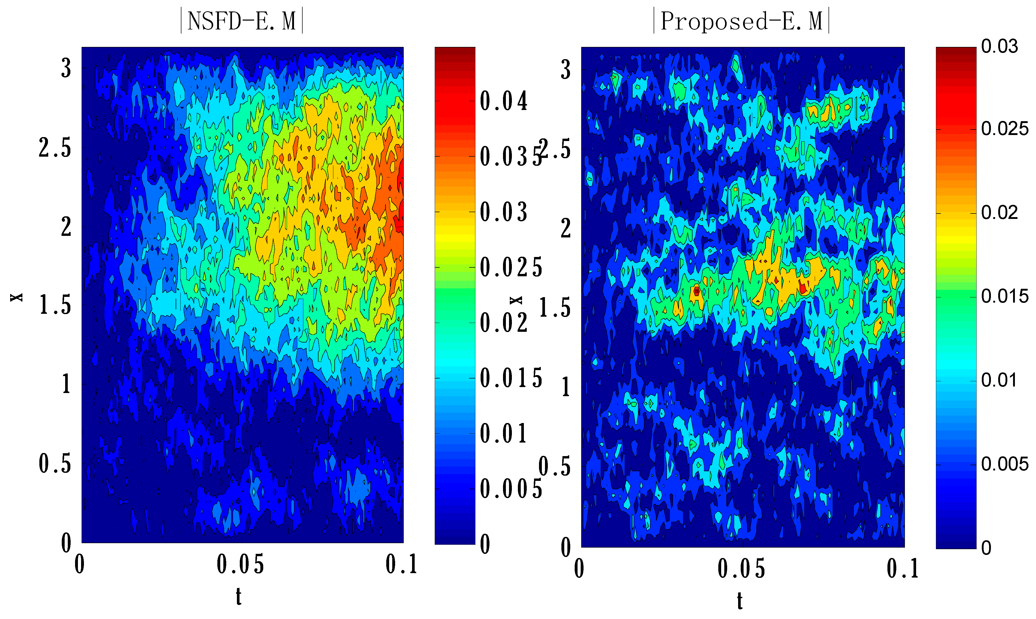
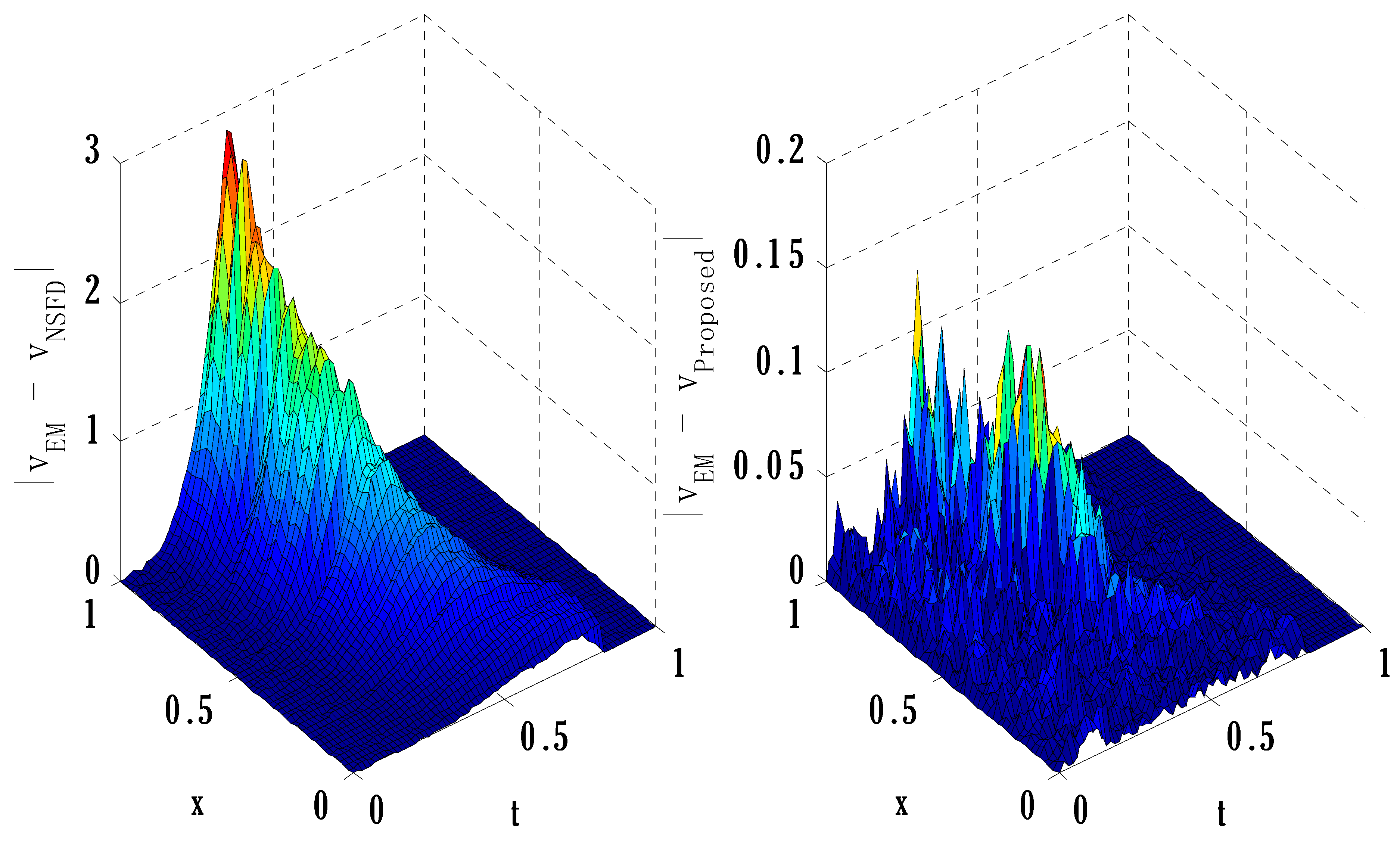
Equations (46)–(48) are solved using the three different finite difference schemes. The whole domain is divided into small portions for finite difference schemes, and time is divided into a finite number of time levels. The step sizes in space and time depend on the number of grid points and time levels. For this example, an additional iterative scheme is not considered. The solution is found explicitly. For the next problem, an additional iterative scheme will be adopted due to handling considered types of boundary conditions. The scheme will require some convergence criteria to stop the iterative solution. One is the Euler–Maruyama, the second is proposed, and the third is the non-standard finite difference method (NSFD). The NSFD has a disadvantage in accuracy but gives unconditional stability. At the same time, the proposed scheme provides the first-order accuracy for stochastic parabolic equations having a constant coefficient of Brownian motion term. The NSFD may produce an accurate solution, but it consumes more time than the proposed one. Figure 1 and Figure 2 are drawn from the solution obtained by Equations (46)–(48) using three schemes. The change in the Wiener process is approximated by the standard normal distribution with a mean of 0 and a standard deviation of t , where t is the temporal step size. The absolute error is calculated by finding the absolute difference between the proposed/NSFD and Euler–Maruyama (E.M) schemes. Contours plots and surface plots are drawn. The difference between the proposed scheme and the Euler–Maruyama scheme is less than the difference obtained by NSFD. The error between the NSFD scheme and the Euler–Maruyama method will grow by choosing a small coefficient of the Wiener process term. Figure 3 shows the deterministic and stochastic solutions of Equations (46)–(48) obtained by three numerical schemes. From Figure 3, it can be observed that the solution obtained by the proposed scheme is closer to the existing Euler–Maruyama scheme, while the solution obtained by NSFD is a bit away from the solution obtained by the Euler–Maruyama method. The comparison of the stochastic proposed scheme and existing stochastic non-standard finite difference method is made by finding L 2 error. The second-order stochastic Runge–Kutta scheme is employed, and the norm for the difference between solutions obtained by the stochastic proposed/NSFD scheme and stochastic second-order Runge–Kutta method is obtained. Table 1 shows the comparison of errors from both schemes. The error obtained by the stochastic proposed scheme is less than that obtained by the existing stochastic NSFD scheme.
Example 2 [42].
Consider the following reaction–diffusion Brusselator model:
d u = d 1 x x u + λ 2 λ 1 + 1 u + u 2 v d t + σ u d W t
d v = d 2 x x v + λ 1 u u 2 v d t + σ v d W t
subject to the initial condition
u 0 , x = 0.5 , v 0 , x = 1 + 5 x
and boundary conditions are given as
d u t , 0 = 0 = d u t , 1 , d v t , 0 = 0 = d v t , 1
where u   a n d   v represent the concentration of the first and second reactant species, respectively; λ 1   a n d   λ 2 denote constant concentration during the chemical process; σ is the controlling parameter; and d 1   a n d   d 2 are diffusion constants.
Equations (49)–(52) are solved by the proposed scheme, and the difference equations are given as
u i n + 1 = u i n + a d 1 u i + 1 n 2 u i n + 1 + u i 1 n x 2 + λ 2 λ 1 + 1 u i n + 1 + u i n 2 v i n d t + σ u i n W
v i n + 1 = v i n + b d 2 v i + 1 n 2 v i n + 1 + v i 1 n x 2 + λ 1 u i n u i n 2 v i n + 1 d t + σ v i n W
where a = d t 1 d 1 d t x 2 d t λ 1 + 1   a n d   b = d t 1 2 d 2 d t Δ x 2 + d t u i n 2 v i n .
The convergence of the proposed scheme depends on the choice of numerical values of parameters and step sizes in space and time. Since the constructed scheme is conditionally stable, it requires suitable step sizes to converge to an accurate solution. However, it converges faster than existing NSFD because it has an order of accuracy more than the existing NSFD method. Since boundary conditions are Neumann-type, an iterative procedure is also adopted. The iterative method requires an initial guess to find the solution at the next iteration. The computational code finds the solution at each time level and each grid point. Furthermore, the same value of the Weiner process is considered for all three schemes for each value of solutions. So, in this manner, a fair comparison is made. The stability region of the proposed and Euler–Maruyama scheme is the same. Still, the proposed scheme has the advantage of providing a positive solution subject to the satisfaction of some inequality. Therefore, the proposed scheme can be more preferred for finding positive solutions to differential equations than the existing Euler–Maruyama scheme. One more advantage of explicit schemes is that they do not require linearization. Therefore, better accuracy might have been achieved when compared with implicit schemes. The positivity of the obtained solution depends on the choice of unknown parameters found using Taylor series expansions.
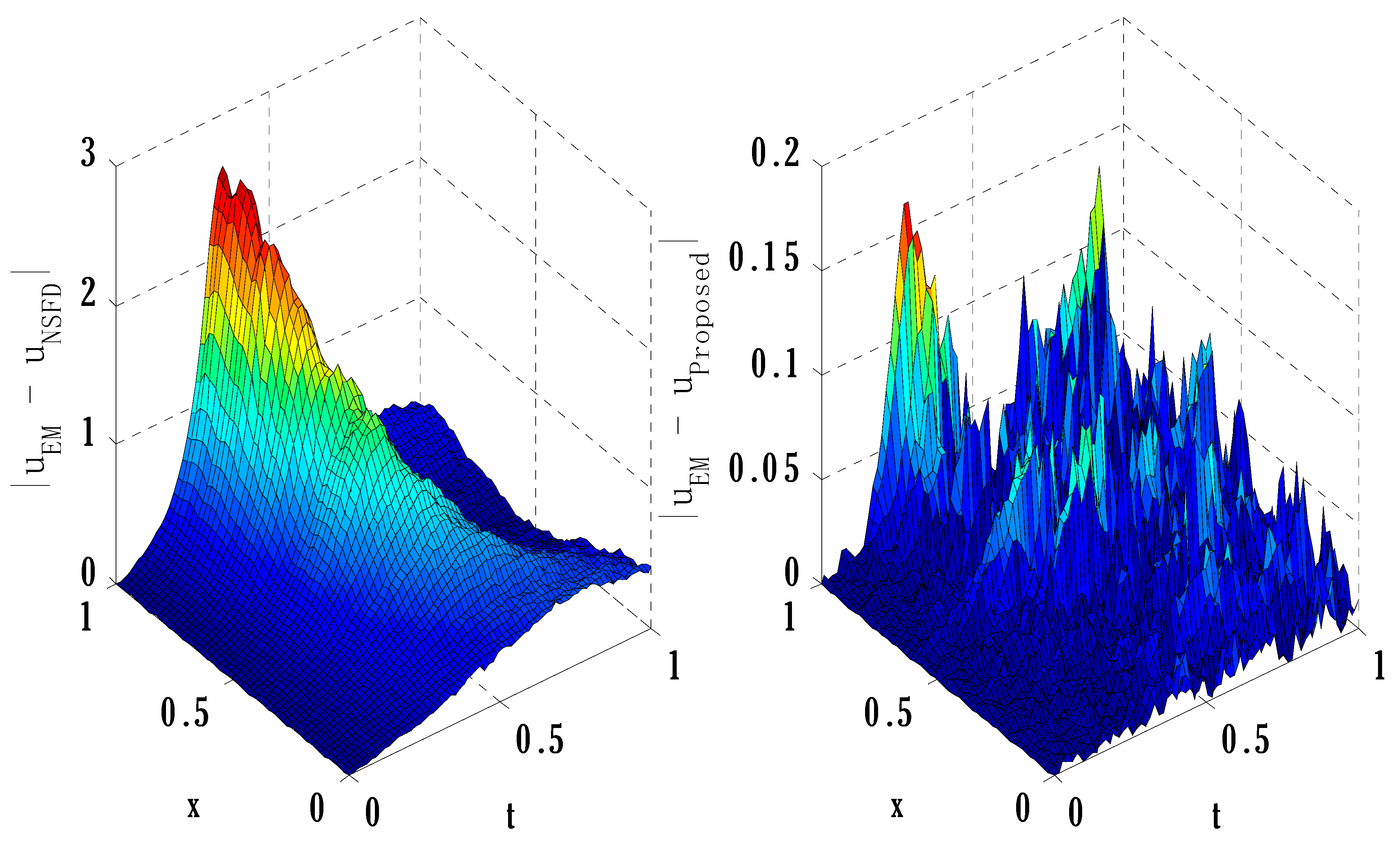
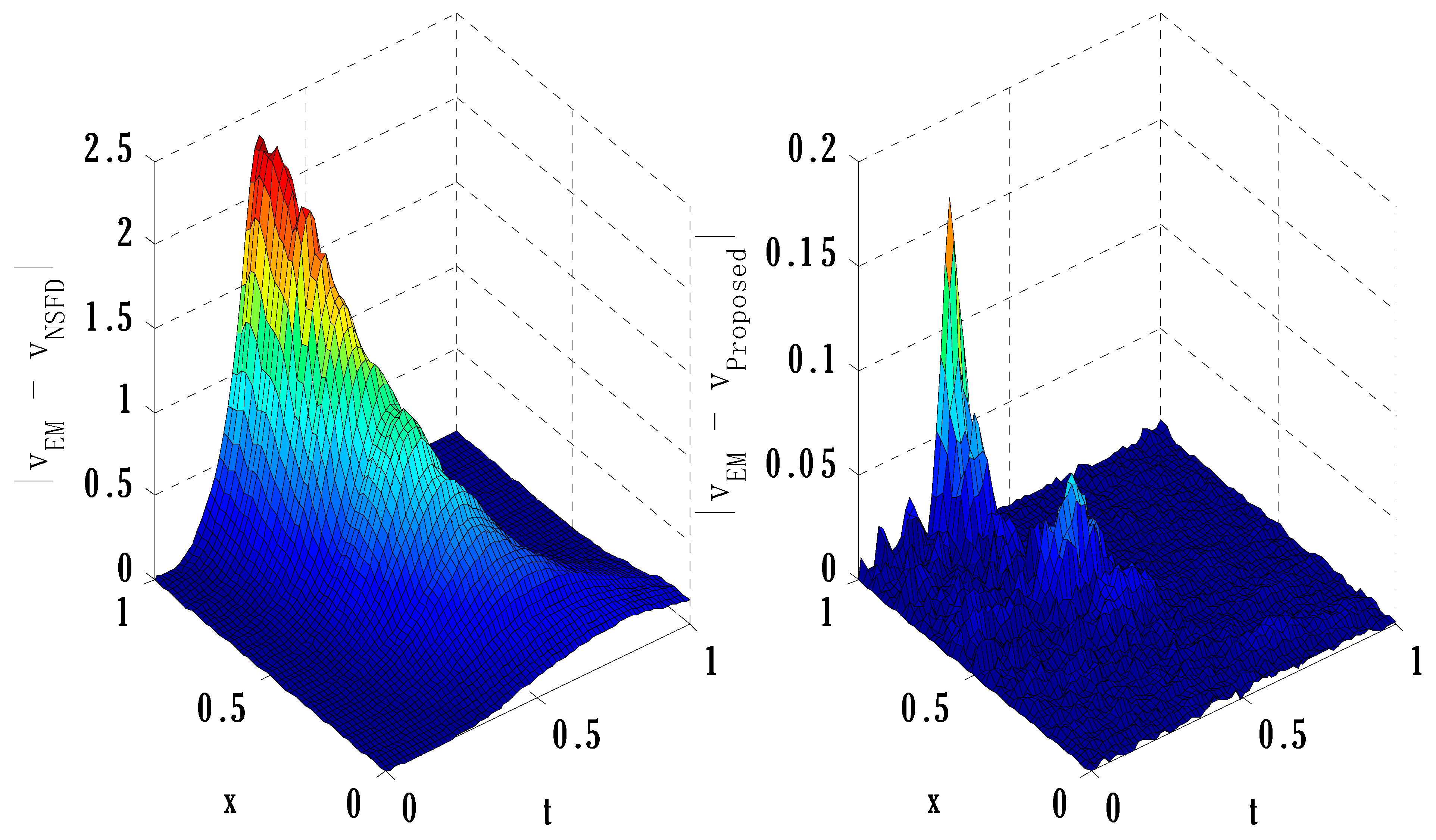
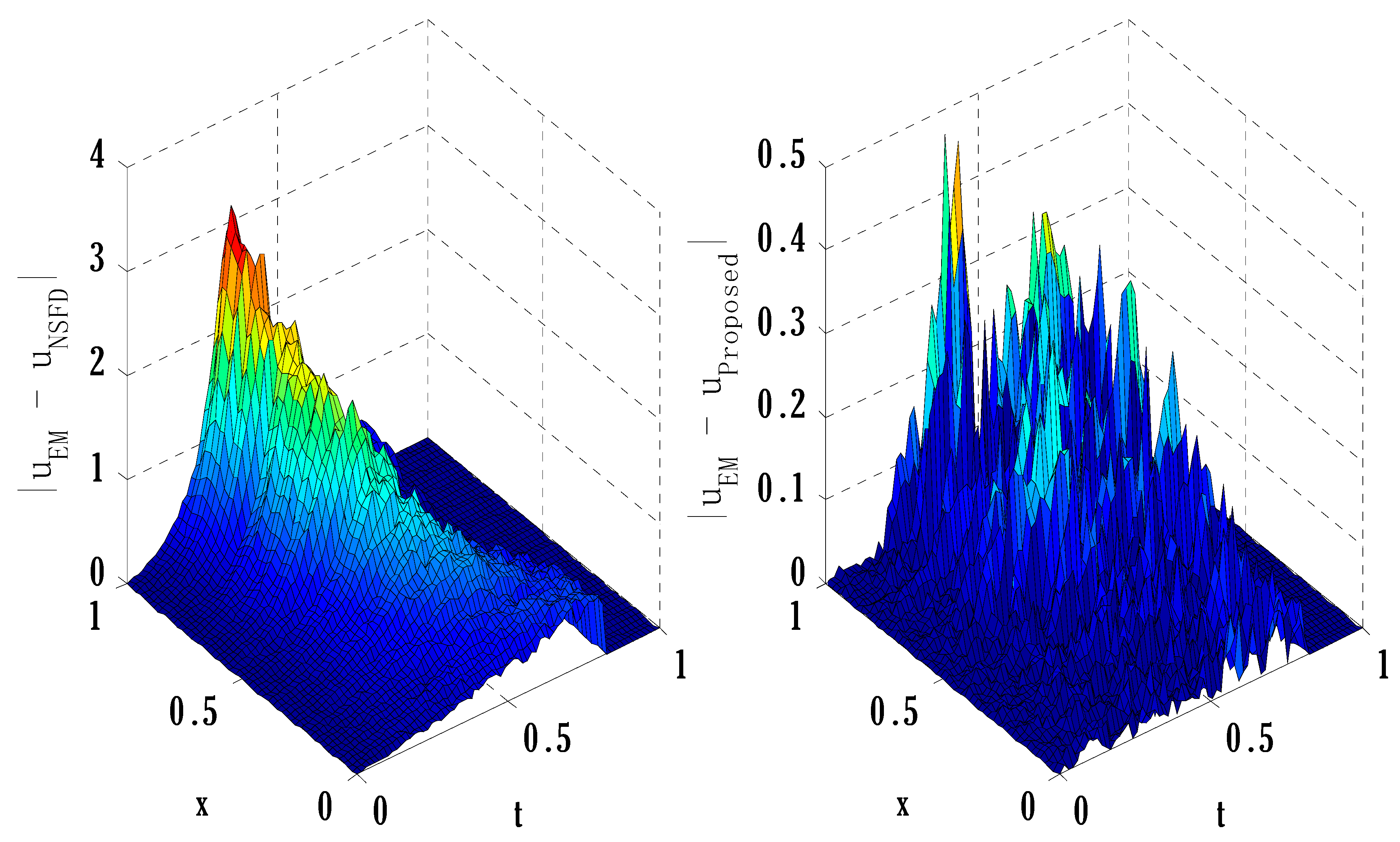
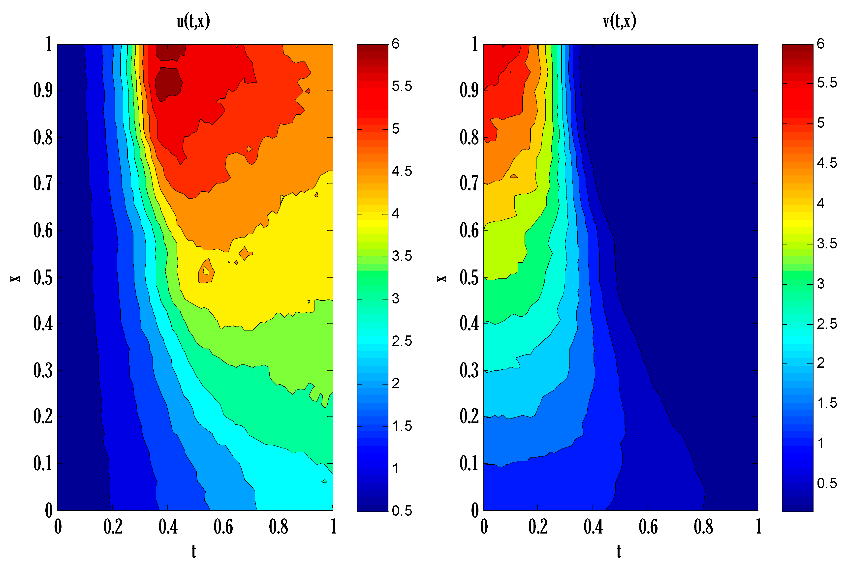
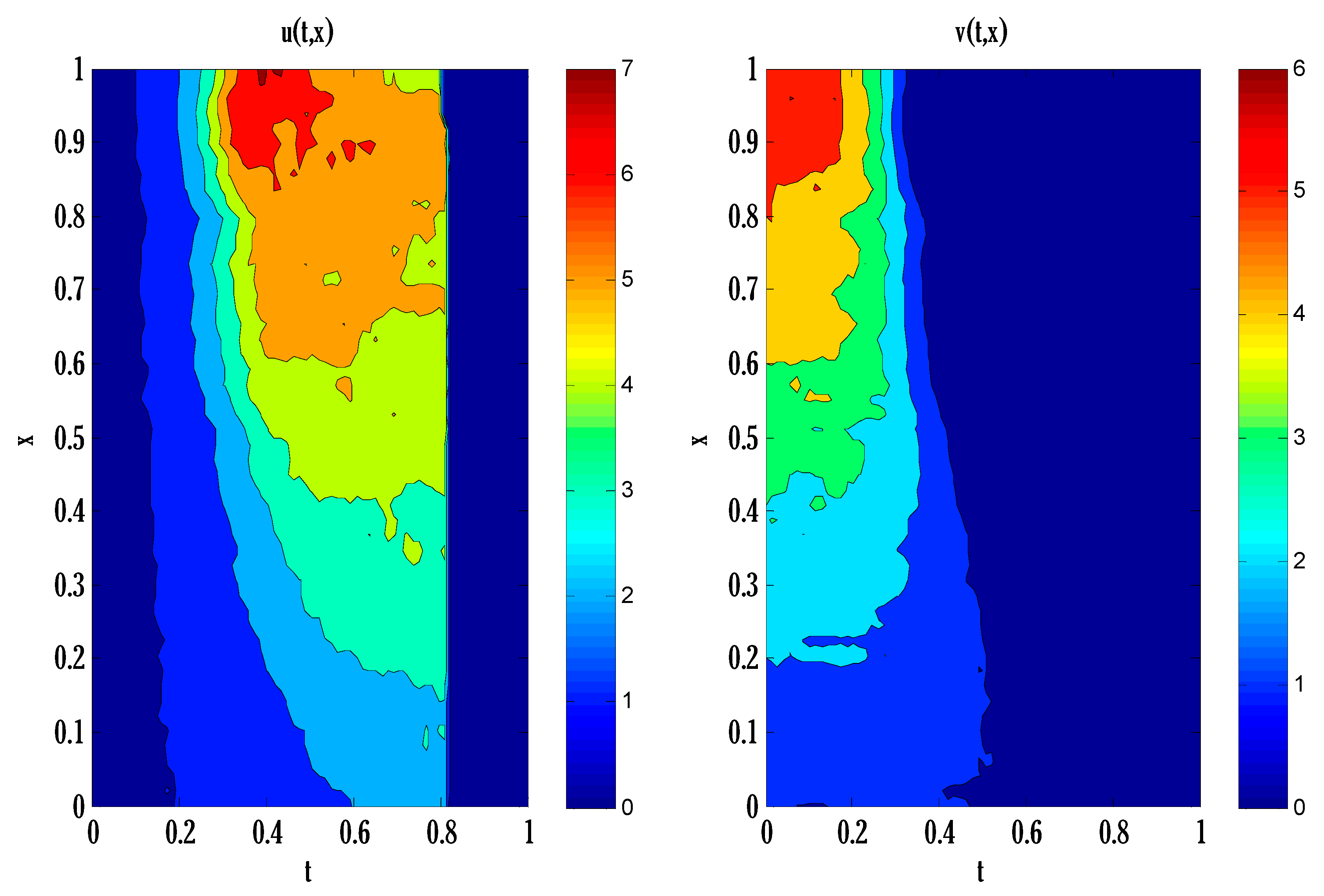
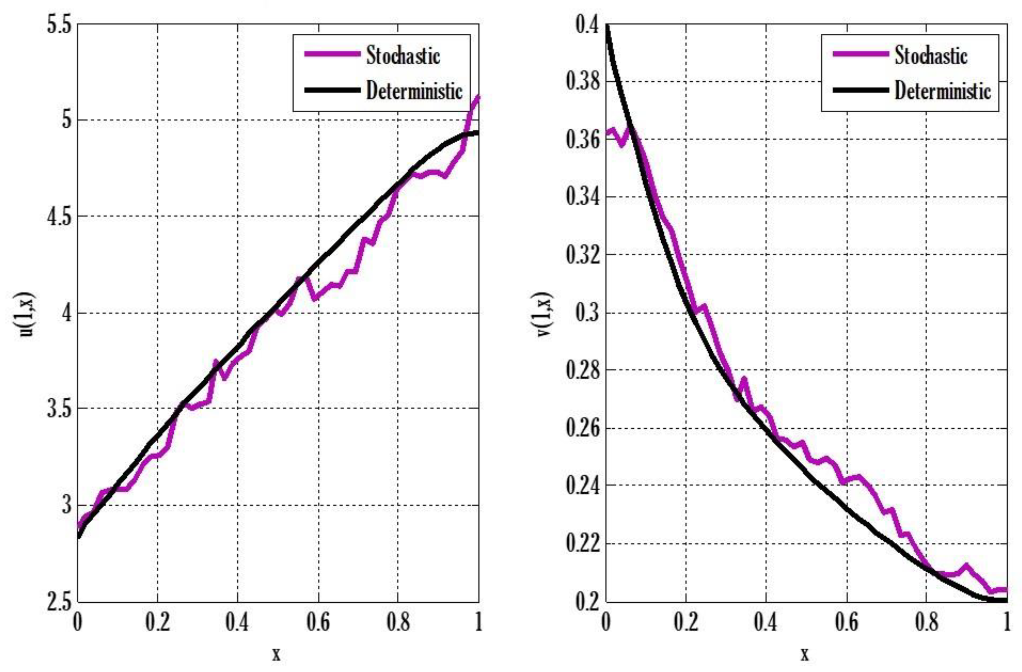
Figure 4, Figure 5 and Figure 6 show the comparison of proposed and NSFD schemes in finding solutions of Equations (46)–(52). From Figure 4, Figure 5 and Figure 6, it can be seen that the proposed scheme produces a smaller absolute error than one obtained by the existing NSFD scheme. Hence, the proposed scheme performs better than the existing NSFD scheme in finding an accurate solution using smaller grid points and time levels. The absolute error is calculated by finding the absolute difference between the proposed/NSFD and the Euler–Maruyama method. Figure 7, Figure 8 and Figure 9 show the contour plots for solutions of Equations (46)–(52) with two values of the controlling parameter, and Figure 10 shows the two-dimensional plot for solutions of Equations (46)–(52). Algorithm 1 is also provided for solving stochastic differential equations using MATLAB. This algorithm also shows how to tackle the stochastic term or Brownian motion term in stochastic differential equations. This strategy is the same as given for the existing Euler–Maruyama method to tackle the Brownian motion term.
Algorithm 1 Pseudo code for the nonlinear problem.
● Input the parameters and independent variables x and t .
● Start the constructing procedure of normal distribution using the command of “makedist,” with a mean of 0 and a variance of Δ t .
● Start the “for” loop for the iterative method and input the initial conditions.
● Start the “for” loops for time and space.
● Input boundary conditions at both ends.
● Use the random of the normal distribution to choose a random value to find the solution of stochastic equations at each grid point and time level using the proposed scheme.
● End the “for” loops for space and time.
● Provide the stopping criteria to stop the iterative method.
● End the iterative “for” loop.

7. Conclusions

A numerical scheme has been constructed to find solutions for stochastic time-dependent PDEs, specially designed for differential equations that provide positive solutions. The scheme has the advantage of providing conditions for positive solutions for those PDEs whose solution must be positive. Both the stability and convergence of the suggested method have been demonstrated. Using Taylor series expansions, the deficiency of the NSFD method has been pointed out and later proved using simulations and the construction of Table 1. Therefore, two strategies have been used to demonstrate that the proposed scheme is more accurate than the NSFD method. Additionally, the scheme has been applied to the scalar and system of stochastic PDEs. The scalar example shows that the proposed scheme produced smaller randomness than Euler–Maruyama and NSFD schemes. After completing this project, we can suggest other applications for the current strategy [43,44,45,46,47,48]. The proposed method not only has a low barrier to entry in terms of its implementation, but it also solves a wider variety of partial differential equations.

Author Contributions

Conceptualization, Y.N.; funding acquisition, K.A.; investigation, Y.N.; methodology, Y.N.; software, Y.N.; formal analysis, Y.N.; writing—review and editing, Y.N.; methodology, M.S.A.; project administration, K.A.; resources, K.A.; supervision, M.S.A.; visualization, K.A.; writing—original draft, M.S.A. All authors have read and agreed to the published version of the manuscript.

Funding

The authors would like to acknowledge the support of Prince Sultan University for paying the Article Processing Charges (APC) of this publication.

Data Availability Statement

The manuscript included all required data and implementing information.

Acknowledgments

The authors wish to express their gratitude to Prince Sultan University for facilitating the publication of this article through the Theoretical and Applied Sciences Lab.

Conflicts of Interest

The authors declare no conflict of interest.

References

  1. Nicolis, G.; Prigogine, I. Fluctuations in nonequilibrium systems. Proc. Natl. Acad. Sci. USA 1971, 68, 2102–2107. [Google Scholar] [CrossRef] [PubMed] [Green Version]
  2. Ahmed, N.; Rafiq, M.; Baleanu, D.; Rehman, M.A. Spatio-temporal numerical modeling of auto-catalytic Brusselator model. Rom. J. Phys. 2019, 64, 110. [Google Scholar]
  3. Ahmed, N.; Baleanu, D.; Korkmaz, A.; Rafiq, M.; Rehman, M.A.; Ali, M. Positivity preserving computational techniques for nonlinear autocatalytic chemical reaction model. Rom. Rep. Phys. 2020, 72, 121. [Google Scholar]
  4. Ahmed, N.; Jawaz, M.; Rafiq, M.; Rehman, M.A.; Ali, M.; Ahmad, M.O. Numerical treatment of an epidemic model withspatial diffusion. J. Appl. Environ. Biol. Sci. 2018, 8, 17–29. [Google Scholar]
  5. Ahmed, N.; S.S., T.; Imran, M.; Rafiq, M.; Rehman, M.A.; Younis, M. Numerical analysis of auto-catalytic glycolysis model. AIP Adv. 2019, 9, 85213. [Google Scholar] [CrossRef] [Green Version]
  6. Yasin, M.W.; Iqbal, M.S.; Ahmed, N.; Akgül, A.; Raza, A.; Rafiq, M.; Riaz, M.B. Numerical scheme and stability analysis of stochastic Fitzhugh-Nagumo model. Results Phys. 2022, 32, 105023. [Google Scholar] [CrossRef]
  7. Arif, M.S.; Abodayeh, K.; Nawaz, Y. A Computational Scheme for Stochastic Non-Newtonian Mixed Convection Nanofluid Flow over Oscillatory Sheet. Energies 2023, 16, 2298. [Google Scholar] [CrossRef]
  8. Fairweather, G.; Meade, D. A survey of spline collocation methods for the numerical solution of differential equations. In Mathematics for Large Scale Computing; CRC Press: Boca Raton, FL, USA, 2020; pp. 297–341. [Google Scholar]
  9. Arqub, O.A.; Al-Smadi, M. Fuzzy conformable fractional differential equations: Novel extended approach and new numerical solutions. Soft Comput. 2020, 24, 12501–12522. [Google Scholar] [CrossRef]
  10. He, J.H.; Ji, F.Y.; Mohammad-Sedighi, H. Difference equation versus differential equation on different scales. Int. J. Numer. Methods Heat Fluid Flow. 2020, 31, 391–401. [Google Scholar] [CrossRef]
  11. Tessitore, G. Existence, uniqueness and space regularity of the adapted solutions of a backward. SPDE Stoch. Anal. Appl. 1996, 14, 461–486. [Google Scholar] [CrossRef]
  12. Dozzi, M.; López-Mimbela, J.A. Finite-time blowup and existence of global positive solutions of a semilinear. SPDE Stoch. Process. Appl. 2010, 120, 767–776. [Google Scholar] [CrossRef] [Green Version]
  13. Xiong, J.; Yang, X. Existence and pathwise uniqueness to an SPDE driven by a-stable colored noise. Stoch. Process. Appl. 2019, 129, 2681–2722. [Google Scholar] [CrossRef]
  14. Altmeyer, R.; Bretschneider, T.; Janák, J.; Reiß, M. Parameter estimation in an SPDE model for cell repolarization SIAM/ASA. J. Uncertain. Quantif. 2022, 10, 179–199. [Google Scholar] [CrossRef]
  15. Gyöngy, I.; Carles, R. On Lp-solutions of semilinear stochastic partial differential equations. Stoch. Process. Appl. 2000, 90, 83–108. [Google Scholar] [CrossRef] [Green Version]
  16. Funaki, T. A stochastic partial differential equation with values in a manifold. J. Funct. Anal. 1992, 109, 257–288. [Google Scholar] [CrossRef] [Green Version]
  17. Mytnik, L. Stochastic partial differential equation driven bystable noise. Probab. Theory Relat. Fields 2002, 123, 157–201. [Google Scholar] [CrossRef]
  18. Zhang, X.; Chen, P.; Abdelmonem, A.; Li, Y. Mild solution of stochastic partial differential equation with nonlocal conditions and noncompact semigroups. Math. Slovaca 2019, 69, 111–124. [Google Scholar] [CrossRef]
  19. Gyöngy, I.; Martínez, T. On numerical solution of stochastic partial differential equations of elliptic type Stochastics: An International. J. Probab. Stoch. Process. 2006, 78, 213–231. [Google Scholar] [CrossRef]
  20. Kamrani, M.; Hosseini, S.M. The role of coefficients of a general SPDE on the stability and convergence of a finite difference method. J. Comput. Appl. Math. 2010, 234, 1426–1434. [Google Scholar] [CrossRef]
  21. Allen, E.J.; Novosel, S.J.; Zhang, Z. Finite element and difference approximation of some linear stochastic partial differential equations. Stoch. Int. J. Probab. Stoch. Process. 1998, 64, 117–142. [Google Scholar] [CrossRef]
  22. Sweilam, N.H.; ElSakout, D.M.; Muttardi, M.M. Numerical solution for stochastic extended Fisher-Kolmogorov equation. Chaos Solitons Fractals 2021, 151, 111213. [Google Scholar] [CrossRef]
  23. Mirzaee, F.; Rezaei, S.; Samadyar, N. Application of combination schemes based on radial basis functions and finite difference to solvestochastic coupled nonlinear time fractional sine-Gordon equations. Comput. Appl. Math. 2022, 41, 10. [Google Scholar] [CrossRef]
  24. Yang, X.; Zhao, W. Strongly convergent error analysis for aspatially semidiscrete approximation of stochastic partial differential equations with non-globally Lipschitz continuous coefficients. J. Comput. Appl. Math. 2021, 384, 113173. [Google Scholar] [CrossRef]
  25. Arezoomandan, M.; Soheili, A.R. Spectral collocation method forstochastic partial differential equations with fractional Brownian motion. J. Comput. Appl. Math. 2021, 389, 113369. [Google Scholar] [CrossRef]
  26. Yasin, M.; Iqbal, M.; Seadawy, A.; Baber, M.; Younis, M.; Rizvi, S. Numerical scheme and analytical solutions to the stochastic nonlinear advection diffusion dynamical model. Int. J. Nonlinear Sci. Nu-Merical Simulation 2021. [Google Scholar] [CrossRef]
  27. Hussain, S.; Tunç, O.; ur Rahman, G.; Khan, H.; Nadia, E. Mathematical analysis of stochastic epidemic model of MERS-corona & application of ergodic theory. Math. Comput. Simul. 2023, 207, 130–150. [Google Scholar] [PubMed]
  28. Alzabut, J.; Alobaidi, G.; Hussain, S.; Madi, E.N.; Khan, H. Stochastic dynamics of influenza infection: Qualitative analysis and numerical results. Math. Biosci. Eng. 2022, 19, 10316–10331. [Google Scholar] [CrossRef]
  29. Wang, Y.; Abdeljawad, T.; Din, A. Modeling the dynamics of stochastic norovirus epidemic model with time delay. FRACTALS 2022, 30, 1–13. [Google Scholar] [CrossRef]
  30. Kruse, R. Consistency and stability of a Milstein-Galerkin finite element scheme for semilinear. SPDE Stoch. Partial. Differ. Equ. Anal. Comput. 2014, 2, 471–516. [Google Scholar] [CrossRef] [Green Version]
  31. Roth, C. A combination of finite difference and Wong-Zakai methods for hyperbolic stochastic partial differential equations. Stoch. Anal. Appl. 2006, 24, 221–240. [Google Scholar] [CrossRef]
  32. Namjoo, M.; Mohebbian, A. Approximation of stochastic partial differential equations with Stochastic Crank-Nicolson method. In Proceedings of the 21st Seminar on Mathematical Analysis and its Applications, Hamedan, Iran, 26–27November 2014. [Google Scholar]
  33. Li, Y.; Mao, X.; Song, Q.; Wu, F.; Yin, G. Strong convergence of Euler-Maruyama schemes for McKean-Vlasov stochastic differential equations under local Lipschitz conditions of state variables. IMA J. Numer. Anal. 2022, 43, 1001–1035. [Google Scholar] [CrossRef]
  34. Hu, L.; Li, X.; Mao, X. Convergence rate and stability of the truncated Euler-Maruyama method forstochastic differential equations. J. Comput. Appl. Math. 2018, 337, 274–289. [Google Scholar] [CrossRef]
  35. El-Metwally, H.; Sohaly, M.A.; Elbaz, I.M. Mean-square stability of the zero equilibrium of the nonlinear delay differential equation: Nicholson’s blowflies application. Nonlinear Dyn. 2021, 105, 1713–1722. [Google Scholar] [CrossRef]
  36. Alshehry, A.S.; Shah, R.; Shah, N.A.; Dassios, I. A Reliable Technique for Solving Fractional Partial Differential Equation. Axioms 2022, 11, 574. [Google Scholar] [CrossRef]
  37. Alderremy, A.A.; Shah, R.; Shah, N.A.; Aly, S.; Nonlaopon, K. Comparison of two modified analytical approaches for the systems of time fractional partial differential equations. AIMS Math. 2023, 8, 7142–7162. [Google Scholar] [CrossRef]
  38. Shah, N.A.; Hamed, Y.S.; Abualnaja, K.M.; Chung, J.-D.; Shah, R.; Khan, A. A Comparative Analysis of Fractional-Order Kaup–Kupershmidt Equation within Different Operators. Symmetry 2022, 14, 986. [Google Scholar] [CrossRef]
  39. Shah, N.A.; Agarwal, P.; Chung, J.D.; El-Zahar, E.R.; Hamed, Y.S. Analysis of Optical Solitons for Nonlinear Schrödinger Equation with Detuning Term by Iterative Transform Method. Symmetry 2020, 12, 1850. [Google Scholar] [CrossRef]
  40. He, W.; Chen, N.; Dassios, I.; Shah, N.A.; Chung, J.D. Fractional System of Korteweg-De Vries Equations via Elzaki Transform. Mathematics 2021, 9, 673. [Google Scholar] [CrossRef]
  41. Yasin, M.; Ahmed, N.; Iqbal, M.S.; Rafiq, M.; Raza, A.; Akgül, A. Reliable numerical analysis for stochastic reaction-diffusion system. Phys. Scr. 2023, 98, 015209. [Google Scholar] [CrossRef]
  42. Iqbal, M.S. Solutions of Boundary Value Problems for Nonlinear Partial Differential Equations by Fixed Point Methods. Doctoral studies of engineering science, Graz University of Technology, Styria, Austria, 21 September 2011. [Google Scholar]
  43. Shatanawi, W.; Raza, A.; Arif, M.S.; Rafiq, M.; Bibi, M.; Mohsin, M. Essential features preserving dynamics of stochastic Dengue model. CMES-Comput. Model. Eng. Sci. 2021, 126, 201–215. [Google Scholar] [CrossRef]
  44. Abodayeh, K.; Raza, A.; Arif, M.S.; Rafiq, M.; Bibi, M.; Mohsin, M. Stochastic numerical analysis for impact of heavy alcohol consumption on transmission dynamics of gonorrhoea epidemic. CMC-Comput. Mater. Contin. 2020, 62, 1125–1142. [Google Scholar] [CrossRef]
  45. Raza, A.; Arif, M.S.; Rafiq, M. A reliable numerical analysis for stochastic gonorrhea epidemic model with treatment effect. Int. J. Biomath. 2019, 12, 1950072. [Google Scholar] [CrossRef]
  46. Arif, M.S.; Raza, A.; Shatanawi, W.; Rafiq, M.; Bibi, M. A stochastic numerical analysis for computer virus model with vertical transmission over the internet. Comput. Mater. Contin. 2019, 61, 1025–1043. [Google Scholar]
  47. Shoaib Arif, M.; Raza, A.; Abodayeh, K.; Rafiq, M.; Bibi, M.; Nazeer, A. A numerical efficient technique for the solution of susceptible infected recovered epidemic model. Comput. Model. Eng. Sci. 2020, 124, 477–491. [Google Scholar] [CrossRef]
  48. Salmon, N.; SenGupta, I. Fractional Barndorff-Nielsen and Shephard model: Applications in variance and volatility swaps, and hedging. Ann. Financ. 2021, 17, 529–558. [Google Scholar] [CrossRef]
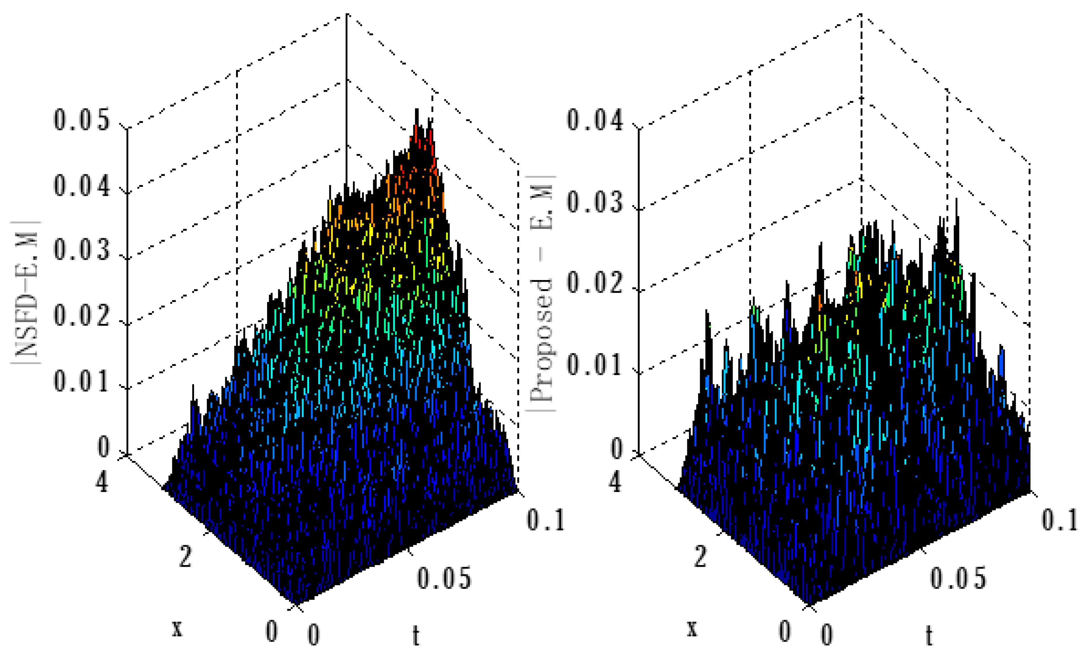
Figure 1. Surface plots for comparison of the proposed scheme with NSFD using N x = 50 ,   N t = 150 ,   σ = 0.4 .
Axioms 12 00460 g001
Figure 2. Contour plots for comparison of the proposed scheme with NSFD using N x = 50 ,   N t = 150 ,   σ = 0.4 .
Axioms 12 00460 g002
Figure 3. Comparison of three schemes using N x = 50 ,   N t = 700 ,   σ = 0.7 .
Axioms 12 00460 g003
Figure 4. Surface plots of u for comparison of the proposed scheme with NSFD using N x = 50 ,   N t = 70 ,   σ = 0.1 ,   λ 1 = 1 ,   λ 2 = 3.4 ,   d 1 = 0.004 ,   d 2 = 0.002 .
Axioms 12 00460 g004
Figure 5. Surface plots for v comparison of the proposed scheme with NSFD using N x = 50 ,   N t = 70 ,   σ = 0.1 ,   λ 1 = 1 ,   λ 2 = 3.4 ,   d 1 = 0.004 ,   d 2 = 0.002 .
Axioms 12 00460 g005
Figure 6. Surface plots of u for comparison of the proposed scheme with NSFD using N x = 50 ,   N t = 70 ,   σ = 0.25 ,   λ 1 = 1 ,   λ 2 = 3.4 ,   d 1 = 0.004 ,   d 2 = 0.002 .
Axioms 12 00460 g006
Figure 7. Surface plots of v for comparison of the proposed scheme with NSFD using N x = 50 ,   N t = 70 ,   σ = 0.25 ,   λ 1 = 1 ,   λ 2 = 3.4 ,   d 1 = 0.004 ,   d 2 = 0.002 .
Axioms 12 00460 g007
Figure 8. Contour plots for solutions u and v using N x = 50 ,   N t = 70 ,   σ = 0.1 ,   λ 1 = 1 ,   λ 2 = 3.4 ,   d 1 = 0.004 ,   d 2 = 0.002 .
Axioms 12 00460 g008
Figure 9. Contour plots for solutions u and v using N x = 50 ,   N t = 70 , σ = 0.25 ,   λ 1 = 1 ,   λ 2 = 3.4 ,   d 1 = 0.004 ,   d 2 = 0.002 .
Axioms 12 00460 g009
Figure 10. Deterministic and stochastic plots for solutions u and v using N x = 50 ,   N t = 70 ,   σ = 0.1 ,   λ 1 = 1 ,   λ 2 = 3.4 ,   d 1 = 0.004 ,   d 2 = 0.002 .
Axioms 12 00460 g010
Table 1. List of L 2 error using σ = 0.1 , L   ( length   of   domain ) = 4 , and t f   ( final   time ) = 0.1 .
N x
N t
L 2 Error
Stochastic ProposedStochastic NSFD
251500.00243.4370
3000.00123.4520
501500.00785.0020
3000.01974.9376
Disclaimer/Publisher’s Note: The statements, opinions and data contained in all publications are solely those of the individual author(s) and contributor(s) and not of MDPI and/or the editor(s). MDPI and/or the editor(s) disclaim responsibility for any injury to people or property resulting from any ideas, methods, instructions or products referred to in the content.