A Modified Simulated Annealing (MSA) Algorithm to Solve the Supplier Selection and Order Quantity Allocation Problem with Non-Linear Freight Rates

Abstract

Economic Order Quantity (EOQ) is an important optimization problem for inventory management with an impact on various industries; however, their mathematical models may be complex with non-convex, non-linear, and non-differentiable objective functions. Metaheuristic algorithms have emerged as powerful tools for solving complex optimization problems (including EOQ). They are iterative search techniques that can efficiently explore large solution spaces and obtain near-optimal solutions. Simulated Annealing (SA) is a widely used metaheuristic method able to avoid local suboptimal solutions. The traditional SA algorithm is based on a single agent, which may result in a low convergence rate for complex problems. This article proposes a modified multiple-agent (population-based) adaptive SA algorithm; the adaptive algorithm imposes a slight attraction of all agents to the current best solution. As a proof of concept, the proposed algorithm was tested on a particular EOQ problem (recently studied in the literature and interesting by itself) in which the objective function is non-linear, non-convex, and non-differentiable. With these new mechanisms, the algorithm allows for the exploration of different regions of the solution space and determines the global optimum in a faster manner. The analysis showed that the proposed algorithm performed well in finding good solutions in a reasonably short amount of time.

1. Introduction

The efficient management of inventory systems plays a crucial role in the success and profitability of businesses across various industries. That is why inventory management is widely studied, and is sometimes called the Economic Order Quantity (EOQ) problem, which aims to determine the optimal order quantity that minimizes the total inventory cost or maximizes the profitability of a certain industry actor. This may include supplier selection and may consider ordering and holding costs, along with other realistic situations [1,2].

The problem may include (as mentioned) the supplier selection, which may be difficult due to the number of requirements to fulfill. For example, suppliers have different capacities (a maximum capacity of produced items per month), different prices, delivery times, and quality indexes. Therefore, supplier selection is an important task in the purchasing activity of the company. Suppliers are usually selected at the same time as the selection of the amount of material purchased from each order and how many orders are placed in the order cycle [3]. Making wise choices may save money when the cost is minimized, or it may help to increase income when the revenue is maximized. Therefore, the task of improving the efficiency of inventory is very important to offer better costs [4,5,6].

Mathematical models are used to perform the aforementioned task. After modeling the process, it is possible to apply optimization techniques to minimize costs or maximize benefits. The mathematical models to be optimized can be complex to solve. Particularly in supplier selection, the objective function is sometimes non-linear, non-convex, and non-differentiable [6]. In some cases, non-linear behaviors are generated by volume discounts. For example, some companies offer discounts on price or transportation costs to encourage customers to purchase larger orders [7,8,9,10].

Traditionally, the EOQ model has been solved using analytical and deterministic methods. However, these methods can struggle to find optimal solutions in complex and realistic scenarios, which often involve multiple items, quantity discounts, maximum capacity on suppliers, etc. [6,7,8,9,10,11,12].

In recent years, the growing importance of computational intelligence has led to the exploration of metaheuristic algorithms to solve complex optimization problems [13]. Metaheuristic methods have been used to solve EOQ problems and demonstrated good efficiency in finding a reasonable solution within a reasonable timeframe.

When the objective function is non-convex (for example, owing to the presence of quantity discounts), traditional methods are more difficult to apply. For example, the classical gradient descent algorithm has been used in supply chain problems [14,15]; however, it performs appropriately only when the objective function is convex.

Metaheuristic methods are a class of iterative, numerical optimization algorithms that utilize probabilistic methods to search for the solution to mathematical problems; they can be used for a wide range of applications, but they have been mainly applied to optimization problems. Although they cannot guarantee to find the global optimal solution, they have been shown to be very powerful in finding a solution near the optimum (and sometimes the optimum) in a very short time, with relatively low computational requirements [13]. That is why they can be used to solve complex problems that are difficult or impossible to solve using traditional optimization methods. Examples of metaheuristic methods include particle swarm optimization (PSO), Genetic Algorithms (GAs), Artificial Bee Colony (ABC) algorithms, and Differential Evolution (DE) [13]. Metaheuristic algorithms have been applied to a wide range of fields, including EOQ problems [2,16].

Simulated Annealing (SA), initially introduced in [17], is one of the most researched metaheuristic optimization algorithms. Inspired by the annealing process of metals, the main advantage of the SA algorithm over other metaheuristic methods is its ability to escape from local suboptimal solutions. This feature makes SA particularly effective for optimization problems with complex, non-convex solution spaces, with suboptimal solutions, where other metaheuristic methods may fail to find the global optimum. These characteristics have motivated the use of SA in several fields of engineering, such as electrical chemistry, mechanics, and operations research [18].

In the supply chain field, the SA algorithm has been used for routing problems. For example, [19] proposed a hybrid heuristic to solve a location-routing problem with two-dimensional loading constraints. The authors of [20] applied Simulated Annealing to solve a model to minimize the total number of connections to transfer passengers and generate flight schedules. This algorithm has been applied to search for the global optimal assembly sequence scheme [21] to find the optimal allocation schemes for water resources [22], scheduling [23], manufacturing systems [24], the traveling salesman problem [25], and others [26,27].

Although the SA algorithm has impressive abilities, it may lead to slower convergence rates, requiring more computation effort to achieve a satisfactory solution.

This paper proposes a Modified Simulated Annealing (MSA) method. The proposed modification consists of utilizing multiple agents and a modified scheme to produce new solutions. The scheme produces a slight attraction to all agents to the current best solution. The MSA contrasts with the traditional SA algorithm, which is usually applied with a single agent. By integrating these new mechanisms, the algorithm is capable of exploring various regions within the solution space and can rapidly identify the global optimum. As a proof of concept, the proposed algorithm was tested with a complex problem that was recently studied in the state of the art, and it is interesting by itself. It is an EOQ problem that considers discounts on transportation costs. The problem has a non-linear, non-convex, and non-differentiable objective function, which is a challenging problem but also good for testing the capabilities of the MSA algorithm. The analysis showed that the proposed algorithm obtained excellent results within a reasonable time. While the previously reported solution (in the scientific literature) took one hour to be obtained, the MSA method obtained ten similar solutions in around one minute. Some of the solutions were even better than the previously reported solution, which means the MSA algorithm discovered new solutions, demonstrating that the previously reported solution is actually a suboptimal solution.

The proposed MSA provided better results in a very short time, compared to the previously reported solution and the traditional SA algorithm, showing that the modifications to the original SA algorithm impacted the results. Furthermore, the presented method represents a novel approach and a unique perspective on the problem. While several multi-agent methods are being developed, little attention has been put on adapting the SA algorithm to work in a multi-agent manner.

The remainder of this paper is organized as follows. Section 2 presents the main definitions of inventory problems and freight rates in transportation costs in the literature, focusing on how the objective function is represented. Section 3 describes the process of the Simulated Annealing method. Section 4 presents the modification of the Simulated Annealing method as a metaheuristic to solve the problem. Section 5 presents computational experiments and analyzes the results when the proposed method was applied. Section 6 presents a discussion and future work, and Section 7 mentions the conclusions.

2. Inventory Problems

Inventory management is an important part of supply chain management. The basic problem statement is as follows. A decision maker must purchase products to store as inventory. Purchasing a larger amount of products may decrease the cost per item for several reasons; for example, every order has a setup cost that is the same regardless of the number of items. If we purchase ten items, the setup cost is split among them. Sometimes the supplier offers a lower cost per item depending on the purchase volume.

On the other hand, storing the items have a (holding) cost if we purchase a large number of items, and selling them takes a longer time. The holding cost increases the cost per item. Solving the EOQ problems involves balancing the costs of holding inventory with the costs of ordering or setup. Economic Order Quantity (EOQ) is a model used in inventory management to mine the optimal inventory level for a business by balancing these costs. 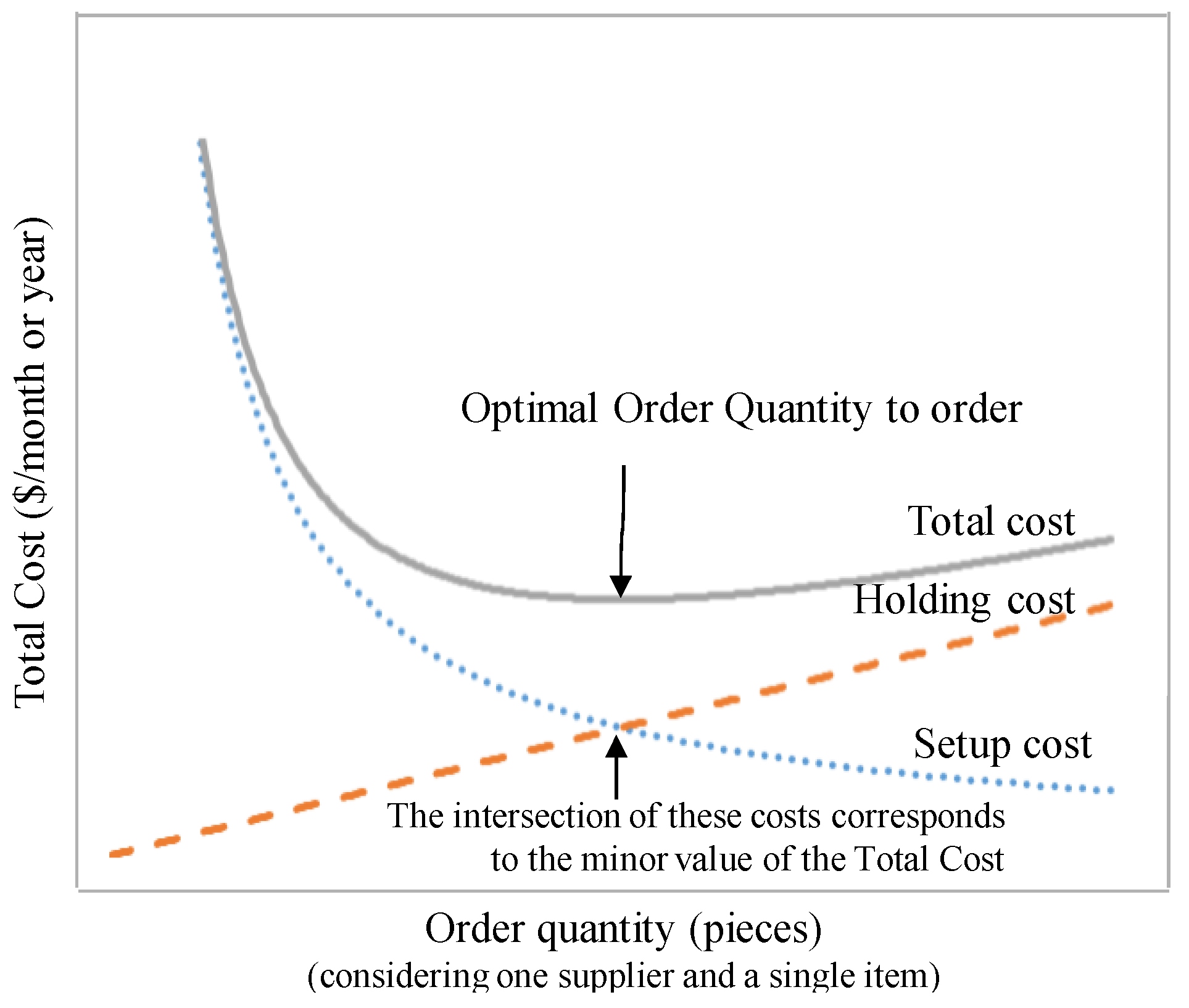Figure 1 shows an example of the discussed problem in which only two variable costs are considered: a constant setup cost (cost for placing an order) and the holding cost.

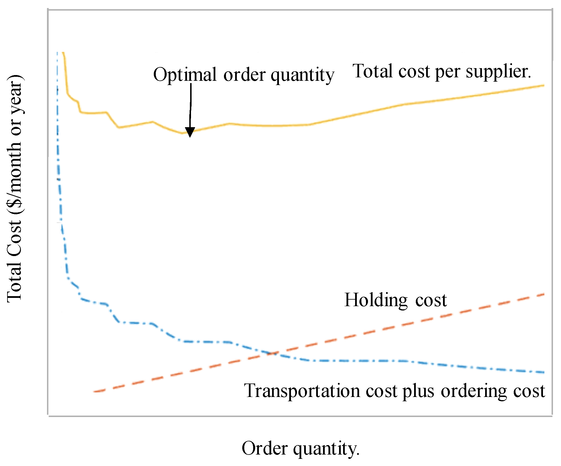
In this type of function, there are no local optimal solutions, and the optimization of the cost has a relatively low complexity. Therefore, it can be solved using classical optimization methods. However, other costs and assumptions will be considered to make this model more realistic. For example, quantity discounts are usually given in a non-linear manner, with thresholds at which the price drops; instead of a formula to calculate the price according to the volume, this kind of discount may be provided by the cost of items or by the shipping cost (or both independently). These discounts introduce local optimal points and produce an objective function that is non-convex, non-linear, and non-differentiable. One example of this is shown in Figure 2.

The complexity of the function increases with the number of suppliers, discounts, and costs. Some of these problems in the literature for supplier selection have been solved using exact methods, which are possible when the number of possible solutions is finite and relatively small. Other authors have also explored other metaheuristic algorithms. Several algorithms have been proposed to solve non-linear problems. There are two different schemes: classical and metaheuristic methods. One classical method is gradient descent, which (as its name indicates) uses a form of gradient descent to solve systems of linear equations. This method is also known as the steepest descent method. This method uses a simple operator to obtain the solution. Some examples of evolutionary methods include the particle swarm optimization (PSO) algorithm, genetic algorithm (GA), and differential evolution (DE) [13]. These methods are searching techniques based on populations [13]. There are other methods based on a single agent, for example, the Simulated Annealing (SA) algorithm, which is a widely recognized technique inspired by the annealing process observed in metallurgy. Devised to tackle complex combinatorial optimization problems, SA emulates the gradual cooling of a material, allowing its atoms to settle into a minimum energy state, forming a highly ordered crystalline structure. By iteratively exploring the solution space and stochastically accepting both improvements and occasional deteriorations, the algorithm strikes a balance between exploration and exploitation, thus increasing the chances of converging to a global optimum.

Owing to its flexibility and effectiveness, the SA algorithm has found success across various domains [13,17]. However, the SA algorithm is a single-agent method, and in recent years, the field of optimization has witnessed a significant shift in focus towards population-based metaheuristic algorithms, as they have steadily gained popularity over traditional single-agent algorithms. This increasing interest can be attributed to several key advantages offered by population-based approaches. Unlike single-agent algorithms, which rely on a single solution’s exploration and exploitation, population-based metaheuristics maintain a diverse set of candidate solutions, promoting global search capabilities and reducing the likelihood of premature convergence to local optima. Additionally, these algorithms are inherently parallelizable [28,29,30], allowing for efficient utilization of modern computational resources and facilitating the solution of large-scale, complex problems.

3. Simulated Annealing (SA) Method

This section introduces the traditional SA method, which is particularly useful in problems where the objective function is non-convex, discontinuous, or noisy. An additional advantage is the simplicity and ease of its implementation.

This method uses a technique that emulates the cooling process of metals. This algorithm is based on gradually decreasing the temperature of a piece of metal to cool it. Kirkpatrick, Gelatt, and Vecchni presented this method in 1983 [17], where, as previously mentioned, temperature reduction in the particles was achieved until the lowest energy state was reached.

Procedure of the Simulated Annealing

To begin the search procedure, an initial solution is generated (can be randomly initialized). This point or initial solution is denoted by x⁰, and this candidate solution is modified in each repetition (iteration). It is also important to define the final number of iterations (Iter). A variable called temperature changes from the initial temperature condition (T₀) to the final temperature (T_e). The rate of change is controlled with a parameter called the cooling rate (ρ).

Beginning with the initial point x⁰, this decision variable must be modified over an iterative process until the number of iterations (Iter) is reached if the temperature is higher than the final temperature. The goal is to converge the algorithm at the end of the process. When the algorithm starts, it uses a high temperature and can explore further areas of the research space. However, through the iterations, the temperature decreases, and the algorithm can explore a smaller region of the research space. Finally, only the solution is modified using the increment Δx of the objective function. An advantage of this algorithm is the use of probability decisions to allow the use of worst solutions to avoid local solutions and increase the exploration process.

After the solution is evaluated in the objective function, let us consider a maximization problem, and the next solution is chosen in two cases:

(i)

First, if the value of the solution is better than the current best solution, the solution is updated.

$$f(x^{k+1})>f(x^k)$$

(1)

In Equation (1), f(x^k) represents the value of the objective function in the current iteration, and f(x^k+1) is the objective function value of the next position x^k+1.

(ii)

The second case involves the use of acceptance probability, $p_a$. This alternative determines that, in some cases, the solution is updated with the new solution, even when the objective function value is smaller (worst for a maximization problem). This mechanism has the purpose of exploring other regions. The solution of the function and its values for the variables is taken if a random value is less than $p_a$. The acceptance probability is calculated using Equation (2).

$$p_a=e^{-\raisebox{1ex}{$\Delta f$}\!\left/ \!\raisebox{-1ex}{$T$}\right.}$$

(2)

where Δf, as was mentioned, represents the increment of the objective function between x^k+1 and x^k.

$$\Delta f=f(x^{k+1})-f(x^k)$$

(3)

When the acceptance probability is calculated, this is compared against a random value (r) that is uniformly distributed between 0 and 1 [0,1]; if r is less than $p_a$, then the next solution x^k+1 is memorized as the new solution.

When the temperature is high (during the first iteration), the acceptance probability is close to 1, and the probability of accepting the new solution is large. However, when the temperature decreases, the acceptance probability is small (close to zero), and the probability of accepting a bad solution is small.

Therefore, temperature plays an important role in this process. The temperature T(k) is updated using the following equation where ρ represents the cooling factor between [0,1], it is a constant value, and the temperature is decremented through the use of this cooling factor.

In the linear scheme, the temperature reduction is calculated using the following equation:

$$T_{k+1}=T_k\rho$$

(4)

Simulated Annealing is a widely used optimization algorithm employed in various fields, including control systems, chemical processes, and structural processes. This algorithm allows engineers to optimize complex systems and algorithms in all these applications, thereby improving their performance and reliability.

Despite its remarkable capacity, Simulated Annealing has slower convergence rates. This is because Simulated Annealing uses a random process to explore the search space, which can result in slower convergence to the optimal solution compared to other methods that use deterministic rules to guide the search.

4. The Modified Simulated Annealing

Simulated Annealing, in its original form, relies on a single solution to explore the search space. Although it has shown good efficiency, for problems with several local suboptimal solutions, this may lead to a low convergence rate. Furthermore, in the field of optimization, population-based algorithms have shown advantages over their single-agent counterparts. Unlike single-agent algorithms, which rely on the exploration and exploitation of a solitary solution, population-based metaheuristics maintain a diverse set of candidate solutions, fostering robust global search capabilities and mitigating the risk of early convergence to local optima. They are also intrinsically parallelizable, enabling efficient use of contemporary computational resources. This is particularly attractive for the SA algorithm in which the searching agent can be (with a low probability) updated with a less optimal solution to prevent a local suboptimal. Multiple agents may reduce the risk of jumping from the global optimal.

Many of the EOQ problems have multimodal and non-linear functions. For example, the decision to choose the best suppliers is an important decision in the industry and needs to be made quickly. For this reason, it is necessary to explore methods that represent a low computational complexity to solve the mathematical models in this topic (supplier selection and order quantity decisions) because these models have a high complexity. Therefore, it is desirable to propose fast and simple algorithms which can be applied to the EOQ problem. This paper presents a modified version of Simulated Annealing to make the algorithm a good tool for exploring multimodal and non-linear functions.

The Modified Simulated Annealing Algorithm

The main objective of the proposed method is to effectively address complex and multimodal objective functions. To achieve this, it is desirable to increase the exploration process and explore more regions of the search space, thereby accelerating the process of finding the optimal solution. To fulfill these requirements, the proposed method incorporates two distinct mechanisms. The first mechanism involves the use of a population of agents instead of just a single agent. By incorporating multiple agents, the algorithm is better equipped to explore different regions of the solution space simultaneously. This approach increases the chances of finding the global optimum in a shorter period of time. The second mechanism involves a new scheme for producing solutions. Rather than simply generating solutions randomly, the proposed method perturbs the solutions with an attraction toward the best value detected so far. This innovative approach allows the algorithm to efficiently navigate the search space and quickly converge on the global optimum. With the incorporation of these new mechanisms, the proposed algorithm can effectively explore different regions of the solution space and determine the global optimum faster. This makes it an ideal tool for solving complex and multimodal objective functions.

To begin the search procedure, the initial points are randomly generated. These points represent the first set of solutions. These solutions are denoted as $x_{ij}^0$. These candidate solutions will be modified in each iteration (Iter) of the process.

To generate the first sets of solutions, the upper and lower limits of the variables must be considered; let us define the lower limit as l and the upper limit as u.

$$x_{ij}^0=l_j+rand(u_j-l_j)$$

(5)

where i represents the number of solution (since the algorithm is initialized with a total number of agents) and j is the decision variable. After the population begins, the solutions are evaluated in terms of the objective function $f(·)$. Among these values, the best solution $x^{best}$ is determined and is considered the optimal solution so far (glob_opt). The next formulation represents the decision criteria for the minimization problem, where ${f(x}_i^k)$ represents the value of the function in the current iteration k for the solution i, and ${f(x}_i^{k+1})$ represents the value of the function in the next iteration k for the solution i. This variable saves the value of the total cost for the solution (agent) i, in the iteration k or k + 1.

Minimization problem decision criteria:

$$f(x_i^{k+1})<f(x_i^k)$$

(6)

The second mechanism incorporated in our algorithm is a new solution generation scheme. Unlike the original SA method, which generates solutions randomly, our scheme introduces perturbations to the solutions while also directing them towards the best value $x^{best}$ identified so far. In the case that a better value than x^best is found, it must be updated. The solutions are then perturbed by considering the following model:

$$\Delta x_i^k=N(0,\sigma T)$$

(7)

$$x_i^{k+1}=x_i^k+\Delta x_i^k\left(x^{best}-x_i^k\right)$$

(8)

An improvement in the algorithm is the gradual reduction of random perturbation $∆x$. The perturbation is generated using a Gaussian distribution $∆x\leftarrow N(0,\sigma T)$; the standard deviation (2.5 for this algorithm) is multiplied by the value of the temperature T. In the first iterations, large random jumps are generated to increase the exploration. As the temperature decreases, the perturbation also decreases. If some variable lies outside the bounds, this perturbance is generated again.

The new solution is accepted, considering the two cases mentioned in a later section. If the objective function value is less than the value for the current solution, an adaptive algorithm is proposed to minimize the cost of the supplier selection process. In the other case, when the value of the objective function is worse, acceptance probability (2) is considered. The new solutions are evaluated in the objective function, and an iterative process is performed until the stop criteria (number of iterations and temperature value) are satisfied. The temperature is then updated as follows:

$$T(k)=T{\rho }^{k+1}$$

(9)

This process is executed iteratively for a number of iterations; therefore, the stop criterion is the maximum number of iterations; when it is achieved, the temperature reaches the final value.

5. The Problem under Study

This section presents the use of the modified Simulated Annealing algorithm to solve the Supplier Selection and Order Quantity Allocation Problem. The algorithm aims to optimize the selection of suppliers and the allocation of order quantities in a way that minimizes the overall cost and meets the demand of the customers.

The problem consists of an inventory manager who needs to purchase a single item to meet a demand of d = 1000 items a month with a perfect rate of q_a = 0.95, which means 5% of items with defective parts are acceptable. Therefore, they must have 950 perfect parts a month.

There are some situations that make the problem complex. There are three (r = 3) possible suppliers (1, 2, and 3) for the items, but none of them can meet the demand of d = 1000 parts a month since their maximum monthly capacity is c₁ = 700, c₂ = 800, and c₃ = 750, respectively. Furthermore, they have different costs per item, different setup costs, and different perfect rates (they cannot offer 100% perfect items). They also have different shipping costs and volume discounts for the shipping cost provided in a non-linear manner, with thresholds at which the cost decreases.

As they have different costs per item (p₁ = 20, p₂ = 24, p₃ = 30), there is the cheapest supplier. However, the cheaper supplier, at least cheaper on the cost per item (USD 20 per item), has a more expensive setup cost (k₁ = 160, k₂ = 140, k₃ = 130), which means it charges the largest amount when making an order (USD 160). Furthermore, as mentioned, suppliers have different perfect rates (q₁ = 0.93, q₂ = 0.95, q₃ = 0.98), which is the percentage of items that meet the specifications (or perfect item), and the cheapest supplier is the worst in this parameter (q₁ = 0.93), which means the supplier offers a perfect rate smaller than the perfect rate required by the customer.

Since the storage is performed in the customer facilities, the holding cost is the same for all items regardless of the supplier (h = USD 10 per item, per month). Notice that this cost is important. If we purchase an item from the cheapest supplier at USD 20 and store it for two months before using it, the cost of this particular item is finally USD 40 (considering only purchasing and holding costs).

The objective is to determine the optimal order quantity to be assigned to each supplier. This function is a non-linear multimodal function with an infinite number of possible solutions and many local suboptimal solutions. Each supplier offers discounts on transportation costs, increasing the complexity of the problem, which is common in the industry. This example was extracted from [31], and for illustrative and comparative purposes, let us use the same example. This problem (in [31]) was solved using the commercial software LINGO as the optimization tool. The parameters are summarized in

Table 1. Parameters of the example problem.

Data	Definition
r = 3	Number of suppliers.
d = 1000	Demand to be met (units per month).
w = 16	Weight of an item shipped (lbs.).
h = 10	Inventory (holding) cost in USD per unit a month.
k1 = 160, k2 = 140, k3 = 130	Setup cost of each supplier in USD per order.
p1 = 20, p2 = 24, p3 = 30	Price of items of the suppliers in USD per unit.
l1 = 1, l2 = 3, l3 = 2	The lead time of the suppliers in days.
q1 = 0.93, q2 = 0.95, q3 = 0.98	The perfect rate of the suppliers.
qa = 0.95	The minimum required perfect rate of the manufacturer.
Y = 30	Time length of the planning scenario in days.
c1 = 700, c2 = 800, c3 = 750	Production capacity of suppliers (units per month)

, and

Table 2. Freight Rates for Suppliers.

Shipped Weight Range (lbs)	Supplier 1	Supplier 2	Supplier 3
1–499	USD 107.75/CWT	USD 136.26/CWT	USD 81.96/CWT
500–999	USD 92.26/CWT	USD 109.87/CWT	USD 74.94/CWT
1000–1999	USD 71.14/CWT	USD 91.61/CWT	USD 61.14/CWT
2000–4999	USD 64.14/CWT	USD 79.45/CWT	USD 49.65/CWT
5000–9999	USD 52.21/CWT	USD 69.91/CWT	USD 39.73/CWT
10,000–19,999	USD 40.11/CWT	USD 54.61/CWT	USD 33.44/CWT
20,000–29,999	USD 27.48/CWT	USD 48.12/CWT	USD 18.36/CWT
30,000–40,000	USD 7525	USD 13,200	USD 5030

shows the freight rates of suppliers.

Each supplier offers a rate for transportation costs, and it is a non-linear function of the shipment weight, which depends on the order size and the weight w of each item. The transportation cost is given in USD per hundred pounds (centi-weight, CWT).

Mendoza and Ventura [32] proposed breakpoints for a continuous piecewise linear function (for the weight shipped). A breakpoint k specifies the point at which a variation in cost occurs. For example, in quantity discounts without over-declaring, there are values for the order quantity that generate a higher transportation cost than a major value for Q. In this situation, the manufacturer should send a major quantity to take advantage of the discount.

5.1. Assumptions of the Problem

• Manufacturers must calculate the quantity assigned per supplier and how often orders are placed (the length of the order cycle).
• The manufacturer must satisfy a demand per period.
• Shortages are not allowed. The demand must be satisfied.
• Assigning each order generates an order cost per supplier. This order cost is independent of the number of pieces purchased; therefore, it is inappropriate to order a small number of items.
• Each supplier sells the items at a different price.
• The lead time indicates how long we must wait from the order assignment until items are received. This should be considered when planning the purchase, but it has no associated cost.
• Each supplier has a different monthly capacity. In this example, no suppliers can produce demand for d = 1000 units per month. This forces the manufacturer to select at least two suppliers, making the problem more challenging.
• Another parameter is the perfect rate of suppliers, which indicates the fraction of non-defective parts over the total purchased units is guaranteed by the supplier. The manufacturer also has a minimum required perfect rate for the total items purchased.
• There is a cost related to the inventory holding cost, which means that the storage of one piece costs several USD. This holding cost is also considered in the transit inventory cost.

This problem implies that the manufacturer pays transportation costs, known as a free-on-board (FOB) policy [31]. It is very important to point out that the transportation cost considers quantity discounts, which introduces a non-linear behavior to the problem and leads to a locally optimal solution. This study considers transportation costs with over-declaring. For example, the transportation cost for the supplier is presented in

Table 3. Actual freight rates considering over-declaring.

Weight Range (lbs)	Freight Rate
1–428	USD 81.96/CWT
429–499	USD 374.7
500–771	USD 74.94/CWT
772–999	USD 611.4
1000–1803	USD 61.14/CWT
1804–1999	USD 993
2000–4070	USD 49.65/CWT
4071–4999	USD 1986.5
5000–7682	USD 39.73/CWT
7683–9999	USD 3344
10,000–13,702	USD 33.44/CWT
13,703–19,999	USD 3672
20,000–27,383	USD 18.36/CWT
27,384–40,000	USD 5030

, and over-declaring is calculated for all suppliers.

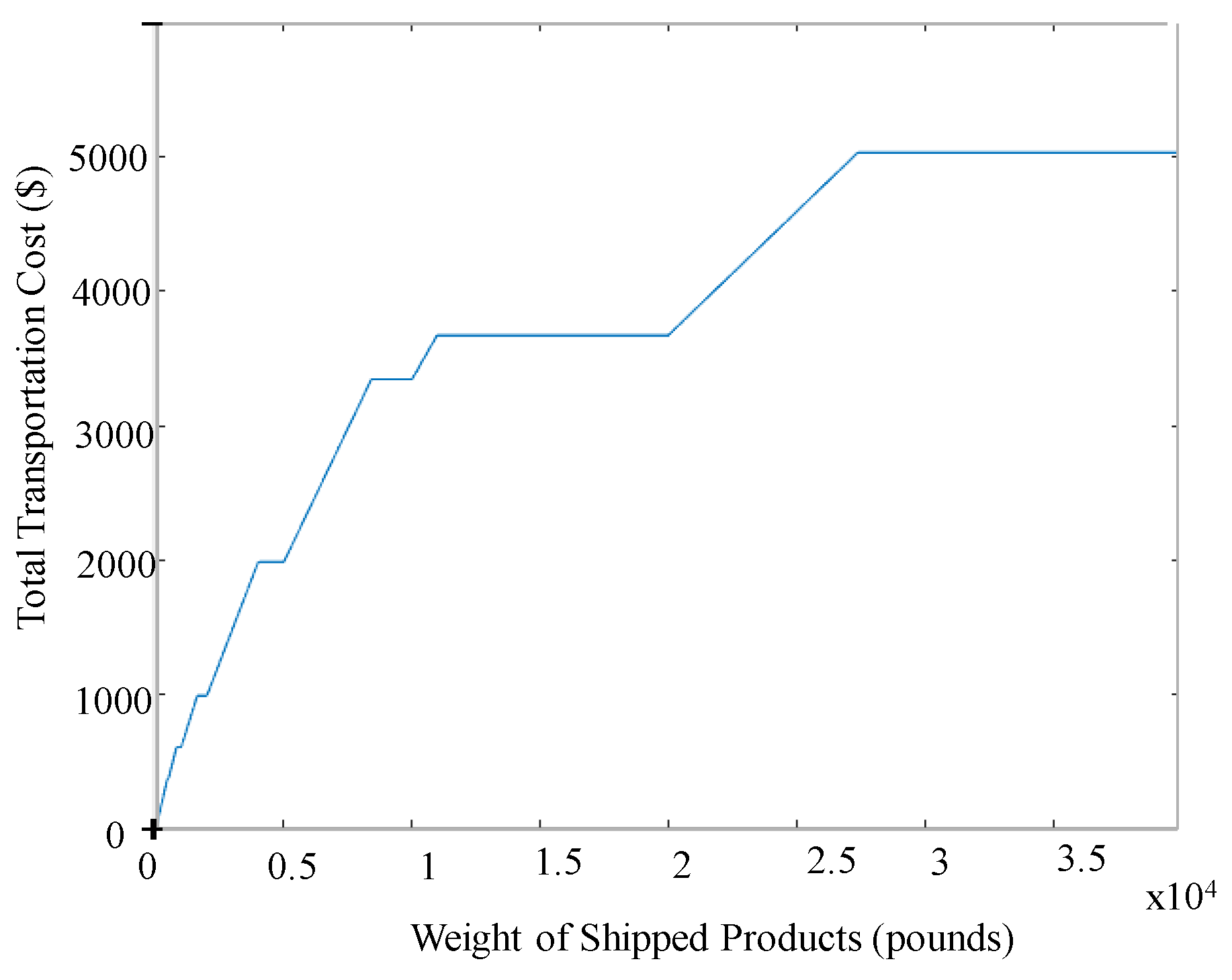
Figure 3 shows the representation of the transportation cost for Supplier 3, using the values from Table 3. It is possible to observe that, in some values for weight, the total transportation cost is the same. With this behavior, the company can take advantage of these circumstances; for example, sending 772 to 999 pounds has the same cost.

5.2. Decision Variables

The variables to be optimized are listed in

Table 4. Solution variables.

Variable	Description
ji	The number of orders assigned to supplier i per order cycle period, ∀ I = 1, …, r.
Qi	The optimal order quantity to supplier i (in units), ∀ i = 1, …, r.
TC	Order cycle period (in months).

, where $j_i$ represents the number of orders assigned per supplier, $Q_i$ represents the optimal order quantity per supplier, and $T_C$ represents the order cycle period.

Before introducing the mathematical model, let us define a couple of variables that will be helpful. First, R_i is the total number of items ordered from the supplier i.

$$R_i=j_i{Q}_i,\forall i=1,\dots ,r.$$

(10)

This definition will be useful when calculating costs that depend on the total number of items ordered from a certain supplier during the full ordera cycle.

The second definition will be the order cycle which is defined as the total items purchased from all suppliers multiplied by their respective perfect rate, divided by the demand multiplied by the required perfect rate.

$$T_C=\frac{{\displaystyle \sum _{i=1}^r{R}_i{q}_i}}{d{q}_a}$$

(11)

5.3. Mathematical Model

The objective function

$$Min{{\rm Z}}_T=\frac{1}{T_C}\left[{\displaystyle \sum _{i=1}^r{j}_i{k}_i+{\displaystyle \sum _{i=1}^r{R}_i{p}_i}+\frac{h}{2d}{\displaystyle \sum _{i=1}^r\frac{R_i^2}{j_i}}+\frac{h}{Y}{\displaystyle \sum _{i=1}^r{R}_i{l}_i}+{\displaystyle \sum _{i=1}^r{j}_{i}TCo{d}_i}}\right],$$

(12)

which is subject to:

$$R_i{q}_{a}d\le c_i{\displaystyle \sum _{i=1}^r{R}_i}{q}_i,\forall i=1,\dots ,r.$$

(13)

$${\displaystyle \sum _{i=1}^r{j}_i=M},$$

(14)

$$j_i\ge 0, \mathrm{integer}, \forall i=1, \dots , r.$$

(15)

$$M\ge 1,\mathrm{integer}.$$

(16)

The objective function (12) calculates the total cost on average, which is why the summation of costs is divided over the order cycle. The summation of costs considers, in the first term, the ordering cost (sum of orders multiplied by the setup cost), the second term calculates purchasing cost (sum of all ordered items multiplied by their respective cost), the third term is the inventory cost (it considers the traditional triangular shape of inventory), the fourth term is the inventory cost in transit (which is also paid by the customer), and finally, the transportation cost. The total cost is calculated per month; thus, the equation is multiplied by the frequency (inverse of the cycle order period). The objective function considers the perfect rate as a part of the order cycle. With this condition, it is possible to ensure the quality requirement, although the supplier’s average quality is less than the minimum perfect rate. Constraint (13) ensures that the assigned order quantity is covered by the supplier’s capacity. Constraint (14) represents the term M, which is the sum of the total number of placed orders.

The order cycle is calculated as:

$$T_c={\displaystyle \sum _{i=1}^r{R}_i{q}_i}/d{q}_a$$

(17)

5.4. Proposed Decision Vector and Parameters of the Proposed Algorithm

The variables to be optimize are represented as a vector for each solution in the algorithm. The vector consists of a set of six quantities (6 dimensions).

$$x_i=\left[\begin{array}{cccccc}{j}_1& j_2& j_3& Q_1& Q_2& Q_3\end{array}\right]$$

(18)

where $j_i$ represents the number of orders assigned per supplier, $Q_i$ represents the optimal order quantity per supplier, and $T_C$ is the order cycle period in months.

The parameters of the algorithms were set for the optimization process. Initial parameters were configured with the following values: the total population was set to 200 individuals (agents), and the maximum number of iterations Iter was set to 100, the initial temperature T₀ = 1, final temperature T_e = 1 × 10⁻¹⁰, and the cooling factor ρ = 0.95.

5.5. Computational Results

This section presents the solutions to the Supplier Selection and Order Quantity Allocation Problem using the proposed algorithm. All the experiments were performed using MATLAB R2021 on a Dell Latitude 5420 laptop with an Intel processor with an 11th Gen Intel(R) Core(TM) i7-1165G7 @ 2.80 GHz 1.69 GHz and 32 GB of installed RAM. The computer has a solid state hard disk with 254 GB and runs with Windows 11 Pro 22H2.

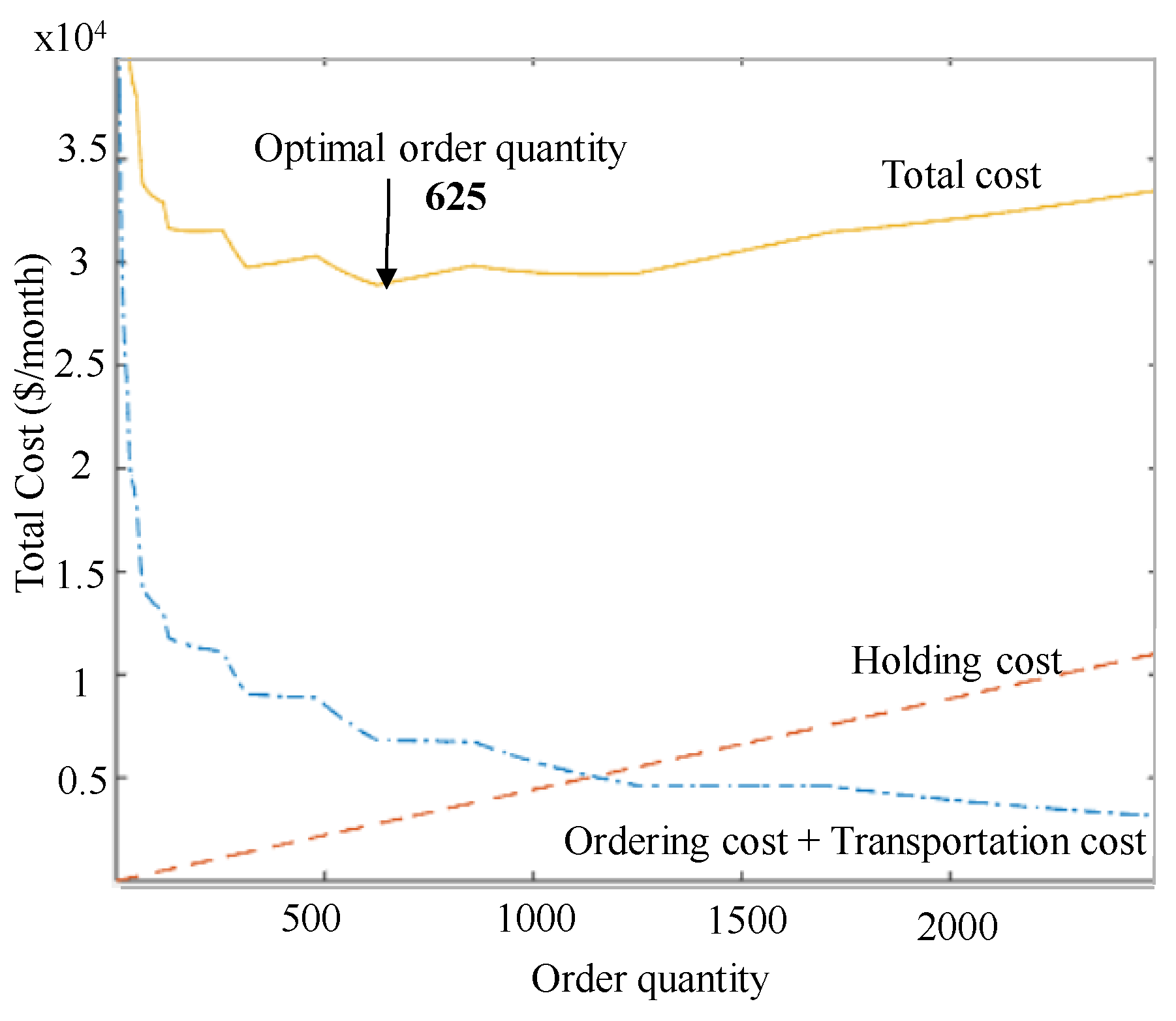
First, the optimal order quantity per supplier was obtained using the modified Simulated Annealing algorithm; for this purpose, only one supplier was considered without considering the capacity constraint; the results per supplier are presented in

Table 5. Optimal solution per supplier.

Sol.	Q	Total Cost (USD/Month)	Ordering Cost	Purchasing Cost	Inventory Cost	Inventory in Transit Cost	Transit Cost
S1	625	USD 28,895	USD 261.50	USD 19,000	USD 2760.9	USD 316.66	USD 6555.6
S2	625	USD 35,532	USD 224	USD 22,800	USD 2820.3	USD 950	USD 8737.6
S3	313	USD 37,155	USD 402.62	USD 28,500	USD 1457.0	USD 633.33	USD 6122.2

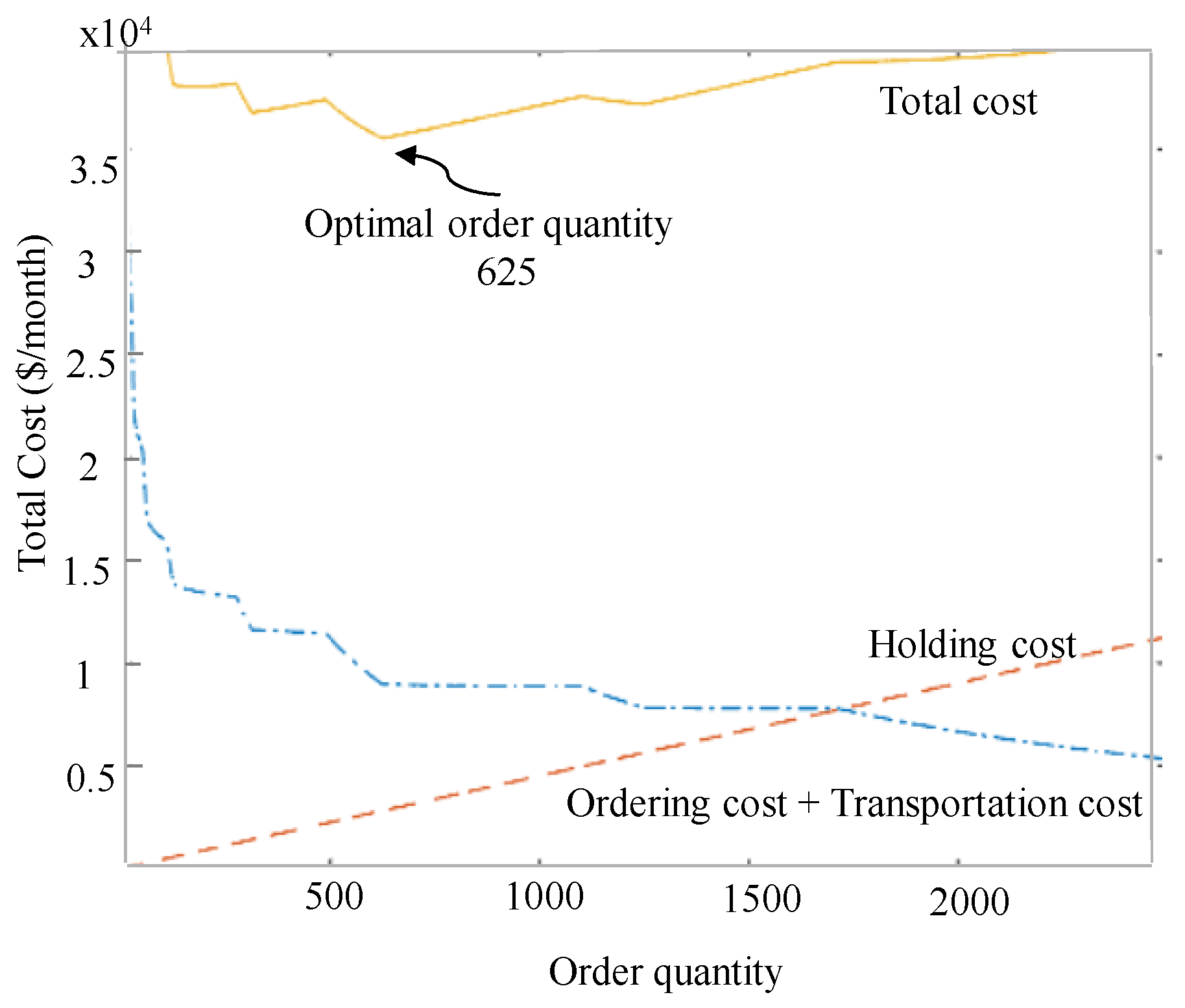
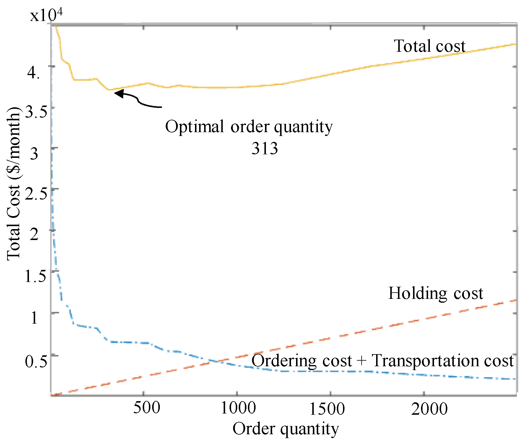
; Figure 4, Figure 5 and Figure 6 represent the total cost against order quantity per supplier, respectively.

In Table 5, it is possible to observe that the cheapest supplier is Supplier 1, and the most expensive one is Supplier 3. Therefore, if the optimization was solved only for one order, the optimal order quantity per supplier is 625, 625, and 313, respectively.

Figure 4, Figure 5 and Figure 6 show the optimal order quantity per supplier, respectively, and the behavior of the costs.

Table 6. Solutions.

Sol	j1	j2	j3	Q1	Q2	Q3	M	Total Cost (USD/Month)	Order Cycle Period (Months)	Time (S)
A	2	1	0	625	625	0	3	USD 32,912.08	1.85	3600
B	6	1	5	652	327	328	12	USD 33,329.99	5.83	5.6
C	5	2	1	625	635	131	8	USD 32,836.84	4.46	8.06
D	6	2	1	625	664	348	9	USD 32,867.77	5.35	5.3
E	9	4	1	625	632	2	14	USD 32,793.15	8.03	4.98
F	10	4	1	625	625	313	15	USD 32,797.14	8.94	7.56
G	9	4	1	625	630	9	14	USD 32,794.64	8.03	9.02
H	8	3	1	625	633	339	12	USD 32,815.16	7.14	8.78
I	2	1	0	640	625	0	3	USD 32,925.76	1.87	5.3
J	5	0	4	640	0	359	9	USD 33,139.79	4.61	9.34
K	4	2	0	631	620	0	6	USD 32,921.87	3.71	5.51

presents the results of several executions using the proposed model of this work for the Supplier Selection and Order Quantity Allocation Problem. It is essential to note that we compared our results with the optimization model presented in reference [31], which was solved using LINGO 17, and the solution is presented in Table 5 as solution $A$ (it was solved with the same computer, the method selected in LINGO package was the Global Optimization).

The solutions labeled as solutions $B$ to $K$, were produced using the proposed model of this work, considering the three suppliers simultaneously. These solutions were generated using the Modified Simulated Annealing algorithm (Section 4) and the parameters were set at the values given in Section 5.4.

The results demonstrate that the majority of the solutions showed a better result than solution $A$. This indicates that the proposed model is effective in optimizing the Supplier Selection and Order Quantity Allocation Problem and can provide superior results compared to the existing optimization model.

As can be seen, our model is easy to develop for the decision-maker and can obtain good solutions in a reasonable amount of time. In contrast, the commercial software LINGO can take several hours to obtain the solution (in LINGO, the stop criteria were set to run for 1 h). This demonstrates that the proposed model is not only effective in producing high-quality solutions but also efficient in terms of computational time and ease of use.

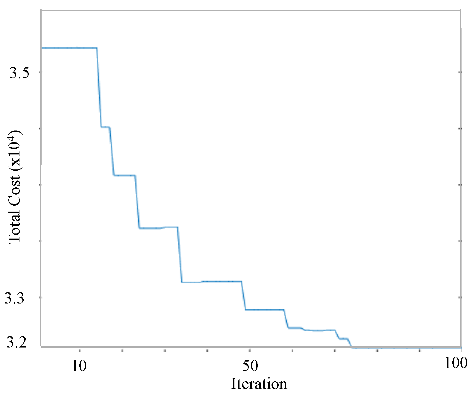
Figure 7 shows the convergence graph for the best solution, E, using Modified Simulated Annealing. In this graph, it is possible to observe that in the first iterations the MSA algorithm performs explorations and obtained large values for the cost; afterwards, as the iterations decrease, the total cost gradually decreased.

The Original Simulated Annealing algorithm was applied with the purpose of comparing it to the proposed algorithm. The parameters were set as initial temperature T₀ = 1, final temperature T_e = 1 × 10⁻¹⁰, and cooling factor ρ = 0.95. Some experimental results are presented in

Table 7. Solutions using Original Simulated Annealing algorithm.

Sol	j1	j2	j3	Q1	Q2	Q3	M	Total Cost (USD/Month)
A	9	6	1	646	448	36	16	USD 33,451.12
B	10	1	4	238	101	250	15	USD 35,184.99
C	9	3	3	549	442	291	15	USD 33,594.07
D	10	1	3	214	464	231	14	USD 35,224.43
E	8	2	3	470	640	178	13	USD 33,931.84
F	10	3	1	634	800	441	14	USD 33,076.23
G	10	2	2	231	372	165	14	USD 34,910.71
H	8	5	2	160	72	106	15	USD 35,769.36
I	6	8	4	632	210	7	18	USD 33,640.92
J	1	7	10	34	144	151	18	USD 39,177.32

.

5.6. Statistical Analysis

In this section, we present a statistical analysis of the Original Simulated Annealing results compared to the Modified Simulated Annealing results. The algorithms were run 30 independent times. A non-parametric statistical technique, the Mann–Whitney test, was applied to test for significance. This statistical test analyzes the equality of medians in two independent samples.

Table 8. Descriptive statistics for SA and MSA.

Algorithm	The Median for the Total Cost	Confidence Interval for the Median 95%, Total Cost (USD/Month)
Original SA	USD 33,522.6	USD 33,066–USD 34,668
Modified SA	USD 32,821.6	USD 32,794–USD 32,911

shows the medians for the two algorithms; with these descriptive statistics, we can observe that the median for the Modified Simulated Annealing algorithm obtained better results.

Table 9. Mann–Whitney test statistics.

Comparison of the Total Cost
Method	W-Value	p-Value	Confidence Interval for the Difference
Adjusted for ties	588	0.00000157	239.39–1134.7
No ties	588	0.00000158

compares the medians of the algorithms to verify if there was a significant difference between the samples. It is possible to observe that the p-value results were favorable, indicating a significant difference.

The results of the Modified Simulated Annealing algorithm were compared against the results obtained from the reference model. A Wilcoxon test was carried out, where results of the 30 independent runs were compared to those of solution A in Table 6 (USD 32,912 presented in [31]).

The results are shown in

Table 10. Wilcoxon test statistics.

Comparison of the Total Cost
Method	Wilcoxon Statistic	p-Value
Modified SA	49	0.019

; it is possible to observe a significant difference between the results from the Modified Simulated Annealing and the state-of-the-art algorithm.

6. Discussion and Future Work

The proposed SA algorithm provided better results in a very short period of time, and while the modifications to the original SA algorithm may appear simple at first glance, they impacted the results. It provided new solutions that were not reported in the previous scientific literature that solved the same problem. Additionally, the results can be obtained in minutes, while commercial software like LINGO may take hours to solve a problem like the one studied in this article. Furthermore, the presented method represents a novel approach and a unique perspective on the problem. While several multi-agent methods are being developed, no attention has been put on adapting the SA algorithm to work in a multi-agent manner.

Future research on this method includes proofs using different state-of-the-art problems, which have been solved with other methods, or the same problem with more variables (for example, more suppliers). The problem solved in this article is a recently studied problem that was selected since its objective function is non-linear, non-differentiable, and non-convex, for which solving this problem is a good proof of concept.

7. Conclusions

This paper proposed a modified Simulated Annealing method. The proposed approach utilizes two distinct mechanisms to enhance its effectiveness in solving complex and multimodal objective functions. Firstly, instead of relying on a single agent, the algorithm employs a population of agents. This allows for the simultaneous exploration of various regions of the solution space, significantly improving the chances of identifying the global optimum within a shorter period of time. Secondly, the method employs a novel solution production scheme that involves perturbing solutions with an attraction towards the best value obtained thus far rather than random generation. This innovative approach enables the algorithm to efficiently navigate the search space and converge more rapidly on the global optimum. By integrating these two mechanisms, the proposed algorithm can efficiently explore different regions of the solution space and determine the global optimum in a shorter period of time. Therefore, it is a highly suitable tool for addressing complex and multimodal objective functions.

To test the performance of the proposed method, it was applied to solve the Supplier Selection and Order Quantity Allocation Problem. For comparison, an instance used in the literature was taken as an example. The instance (with six dimensions) was previously solved using the commercial software LINGO, and a solution was previously reported.

The numerical results showed that the proposed algorithm was able to find the solution in a very short amount of time compared to the LINGO method. The proposed method found solutions in the range of 5.3 to 9.34 s, while LINGO took one hour; the worst case in the proposed method took only 0.26% of the time needed by the commercial software, and some of the solutions were even cheaper than the previously reported solution, leading to a better solution for the example problem.