Article

Nonparametric Directional Dependence Estimation and Its Application to Cryptocurrency

1
Department of Statistics, Sookmyung Women’s University, Seoul 04310, Republic of Korea
2
John Molson School of Business, Concordia University, Montreal, QC H3H 0A1, Canada
3
Statistics Discipline, University of Minnesota-Morris, Morris, MN 56267, USA
*
Author to whom correspondence should be addressed.
Axioms 2023, 12(3), 293; https://doi.org/10.3390/axioms12030293
Submission received: 16 February 2023 / Revised: 6 March 2023 / Accepted: 10 March 2023 / Published: 11 March 2023
(This article belongs to the Special Issue Statistical Methods and Applications)

Abstract

:
This paper proposes a nonparametric directional dependence by using the local polynomial regression technique. With data generated from a bivariate copula having a nonmonotone regression structure, we show that our nonparametric directional dependence is superior to the copula directional dependence method in terms of the root-mean-square error. To validate the directional dependence with real data, we use the log returns of daily prices of Bitcoin, Ethereum, Ripple, and Stellar. We conclude that our nonparametric directional dependence, by using the local polynomial regression technique with asymmetric-threshold GARCH models for marginal distributions, detects the directional dependence better than the copula directional dependence method by an asymmetric GARCH model.

1. Introduction

Since the COVID-19 pandemic, chaos and uncertainty in the financial market has been rising rapidly, resulting in investors having difficulty with the risk management of their financial portfolios. The authors in [1] studied the relationship between cryptocurrency price and the price of stock and gold using copulas. The copula function is useful as it relaxes the assumptions of normality, linearity, and independence of the residuals [2]. In particular, the application of the copula method in economics and finance is explained well in [3,4,5,6,7,8,9,10,11,12]
Gaussian copula marginal regression (GCMR) was proposed by [13], and a beta regression model to analyze bounded time series was proposed by [14]. With the GCMR method, copula directional dependence methods by asymmetric generalized autoregressive conditional heteroskedasticity (GARCH) and stochastic volatility models were developed by [15,16]. For the applications of the copula directional dependence model to cryptocurrency, the copula directional dependence using neural network models was applied to four major cryptocurrencies: Bitcoin (BTC), Ethereum (ETH), Stella (XLM), and Ripple (XRP) [17]. However, the copula directional dependence uses the logit function, so it has difficulty detecting directional dependence when the data have an extremely nonlinear pattern. The purpose of this research was to propose a versatile and flexible directional dependence for all kinds of data patterns by using an optimized nonparametric method.
The novelty of this paper is that we are the first to apply a nonparametric method to directional dependence. The contribution of this paper is that our proposed nonparametric directional dependence method can detect nonlinear pattern directional dependence better than the current copula directional dependence or traditional linear regression directional dependence.
The remainder of this review paper is organized as follows: Section 2 describes the copula directional dependence. In Section 3, we explain our nonparametric directional dependence and present a numerical study. To verify the proposed directional dependence, a real data illustration with four cryptocurrencies is given in Section 4. Finally, conclusions are presented in Section 5.

2. Copula and Directional Dependence

A d-dimensional copula C is a multivariate joint distribution function associated with uniformly distributed marginals. In this article, we focus on a bivariate copula ( n = 2 ). Let F X , Y ( x , y ) be the joint distribution function of a random vector ( X , Y ) with marginal distributions F X and F Y , respectively. According to Sklar’s theorem [2], the distribution of F X , Y can be represented as F X , Y ( x , y ) = C ( F X ( x ) , F Y ( y ) ) for some copula C. Actually, the copula C ( u , v ) is a joint distribution function of U = F X ( X ) and V = F Y ( Y ) . Let r V | U ( u ) denote the conditional expectation of V given U = u . Using the regression function r V | U ( u ) , ref. [18] defined a directional dependence from X to Y:
ρ X Y 2 = V a r ( r V | U ( U ) ) V a r ( V ) = 12 V a r ( r V | U ( U ) ) .
In a similar way, we can define a directional dependence from Y to X:
ρ Y X 2 = V a r ( r U | V ( V ) ) V a r ( U ) = 12 V a r ( r U | V ( V ) ) .
Note that ρ X Y 2 is the nonparametric R-squared between U and V, which was proposed in [19]. Since the influence of the marginals has been eliminated in U and V, we can interpret ρ X Y 2 as the margin-adjusted nonparametric R-squared. The two directional dependence measures ρ X Y 2 and ρ Y X 2 can be used to identify the stronger direction, i.e., a larger value indicates a stronger direction of influence.
To estimate the directional dependence, ref. [15] assumed a specific parametric form of the copula regression function. Concerning the random variables U = F X ( X ) and V = F Y ( Y ) , they assumed that V i given U i = u i followed a beta distribution B e t a ( μ i , κ i ) with the mean parameter 0 < μ i < 1 and the precision parameter κ i > 0 . Specifically, the density function of V i | U i = u i was written as
f ( v i ; μ i , κ i ) = Γ ( κ i ) Γ ( μ i κ i ) Γ ( ( 1 μ i ) κ i ) v i μ i κ i 1 ( 1 v i ) ( 1 μ i ) κ i 1 ,
where Γ ( · ) is the gamma function. They assumed that the mean parameter μ i = E ( V i | U i = u i ) was linked with the covariate u i through a logit function
log μ i 1 μ i = β 0 + β 1 u i
and the precision parameter κ i was given as κ i = 1 + exp ( β 0 + β 1 u i ) . They proposed to estimate the parameters ( β 0 , β 1 ) using the maximum likelihood method of GCMR [13,20]. Then, the directional dependence ρ X Y 2 could be estimated as the sample variance of μ ^ i = exp ( β ^ 0 + β ^ 1 u i ) / ( 1 + exp ( β ^ 0 + β ^ 1 u i ) ) divided by the sample variance of u i . ρ Y X 2 could be estimated in a similar way. When transforming the given data ( x i , y i ) into uniform data ( u i , v i ) , the empirical distribution function was used. The approach of [15] assumed that the regression functions defined between the transformed variables (U and V) had the form of a logistic curve, which is monotonic and has rotational symmetry. This assumption distorted the estimation of copula directional dependence, especially when the regression function was not a monotonic function. In Section 3, we show through numerical studies that their method has this issue in the estimation of the copula directional dependence in certain cases. The authors of [15] assumed that the uniform variable V had a conditional distribution V | U = u , which followed a beta distribution B e t a ( μ u , κ u ) with the mean parameter μ u = E ( V | U = u ) = exp ( β 0 + β 1 u ) / ( 1 + exp ( β 0 + β 1 u ) ) and the precision parameter κ u = 1 + exp ( β 0 + β 1 u ) . In our numerical study, instead of assuming a specific form of the regression function, we simply estimate r V | U ( u ) = E ( V | U = u ) using the local polynomial regression technique [21]. Then, we estimate ρ X Y 2 as the sample variance of r ^ V | U ( u i ) divided by the sample variance of u i .

3. Nonparametric Directional Dependence and Numerical Study

In our simulation, we assumed that the data were uniform, thus negating the need to convert it to a uniform distribution. We considered two scenarios. The first one was the case where the regression function between the transformed variables was monotonic, so the approach of [15] was expected to work well. The second one was the case where the regression function between the transformed variables was nonmonotonic.
In the first scenario, we generated data from an asymmetric copula distribution, which was constructed by combining two symmetric copulas [22] as
C α , β ( u , v ) = A θ 1 ( u α , v β ) A θ 2 ( u α ¯ , v β ¯ ) ,
where 0 < α , β < 1 , α ¯ = 1 α , β ¯ = 1 β , and A θ ( u , v ) is a Plackett copula with parameter θ > 0 (Plackett, 1965). For the simulation, we set θ 1 = 5000 , θ 2 = 5 , α = 0.9 , and β = 0.2 . Figure 1 shows the two regression functions between the transformed variables with their best approximations using logistic curves (in terms of L 2 -distance). Note that both functions are monotonic but the regression function E ( U | V = V ) was better approximated than the function E ( V | U = u ) . The directional dependence measures were ρ U V 2 = 0.1759 and ρ V U 2 = 0.1242 .
In the second scenario, we generated uniform data from a bivariate copula with a nonmonotone regression structure referring to the work of [23]. Ref. [23] devised a method to modify a bivariate copula family so that it had a nonmonotone regression structure using an appropriate measure-preserving function f : [ 0 , 1 ] [ 0 , 1 ] that characterized the dependence structure. We chose f ( x ) = 3 x I ( 0 x 1 / 3 ) + ( ( 3 / 2 ) x + 3 / 2 ) I ( 1 / 3 x 1 ) , where I ( · ) is an indicator function and modified a normal copula with parameter ρ = 0.5 . Note that the nonmonotonicity of the measure-preserving function f ( x ) produces a nonmonotone regression function. The detailed steps of the modification are described as follows (Section 3 of [23]):
(1)
Choose a measure-preserving function f : [ 0 , 1 ] [ 0 , 1 ] that captures the desired dependence structure.
(2)
Choose a parametric family of copulas { C α : α is a copula parameter } (the copulas C α admit densities ϕ α ).
(3)
The resulting copula density function is given as p α ( u 1 , u 2 ) = ϕ α ( f ( x 1 ) , x 2 ) and the corresponding distribution function is given as D α ( u 1 , u 2 ) = 0 u 1 0 u 2 p α ( s 1 , s 2 ) d s 1 d s 2 .
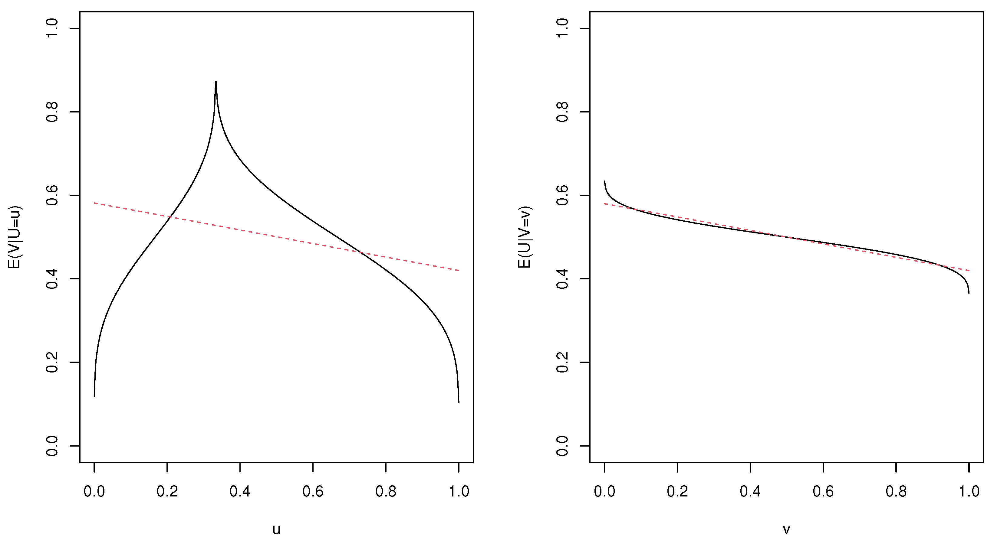
Figure 2 shows the two regression functions between the transformed variables with their best approximations using logistic curves (in terms of L 2 -distance). Note that the function E ( U | V = v ) is monotonic but the function E ( V | U = u ) is not monotonic. Hence, the function E ( V | U = u ) was not approximated by a logistic curve. Even the best approximation showed significant differences from the original function. The directional dependence measures were ρ U V 2 = 0.2394 and ρ V U 2 = 0.0267 . Because of the monotonicity constraint, ref. [15]’s method was expected to have difficulties in estimating the directional dependence from U to V ( ρ U V 2 ).
For the implementation of the copula directional dependence method by [15] (referred to as copula DD method hereafter), we used the R package gcmr, which also supports beta regressions. Through communication with the authors of [15], we learned that in their simulations they set κ as a constant. Therefore, we set the precision parameter κ to be constant as in their simulations. To implement the alternate estimation method using the local polynomial regression, we used the normal kernel and set the degree to be one (local linear estimator). For the bandwidth selection, we computed the plug-in-bandwidth selector implemented in the R package locpol.
Table 1 and Table 2 show the simulation results. Under the first scenario, the two methods seemed to work well. The root-mean-square errors decreased as the sample size increased. However, under the second scenario, the copula method did not work when estimating the directional dependence from U to V. The reason was that the regression function could not be approximated using logistic curves as shown in the left panel of Figure 2. The proposed estimator did not suffer from such problems as expected.

4. Real Data Illustration

We wanted to show that the nonparametric directional dependence method performed better than the copula directional dependence method for financial market data. We applied both copula and nonparametric methods for the directional dependence to cryptocurrency data. Cryptocurrency is a digital currency that does not rely on any central authority to uphold or maintain it. Due to advances in computer technology, such as blockchain and cloud computing, the number of cryptocurrencies has rapidly increased. The rise of cryptocurrencies has led to many investors including cryptocurrencies in their financial portfolios.
Based on a high market cap and cryptocurrencies’ initial offering history, we chose Bitcoin (BTC was created in 2009 and has a $ 431 , 130 , 583 , 788 market cap), Ethereum (ETH was created in 2015 and has a $ 191 , 357 , 725 , 770 market cap), Ripple (XRP was created in 2012 and has a $ 19 , 151 , 338 , 397 market cap), and Stellar (XLM was created in 2015 and has a $ 2 , 227 , 918 , 509 market cap). We collected BTC, ETH, XRP, and XLM daily prices from 1 July 2016 to 23 June 2021 from the following website (https://coinmarketcap.com/, accessed on 24 June 2021). We focused on the log return of the four cryptocurrency prices (in percentages) instead of the original prices. To eliminate the serial dependence of a given time series data, we fit the asymmetric threshold-GARCH (1,1) model to the log return data, generated standard residuals, and then transformed them to the uniformly distributed data using the empirical distribution function.
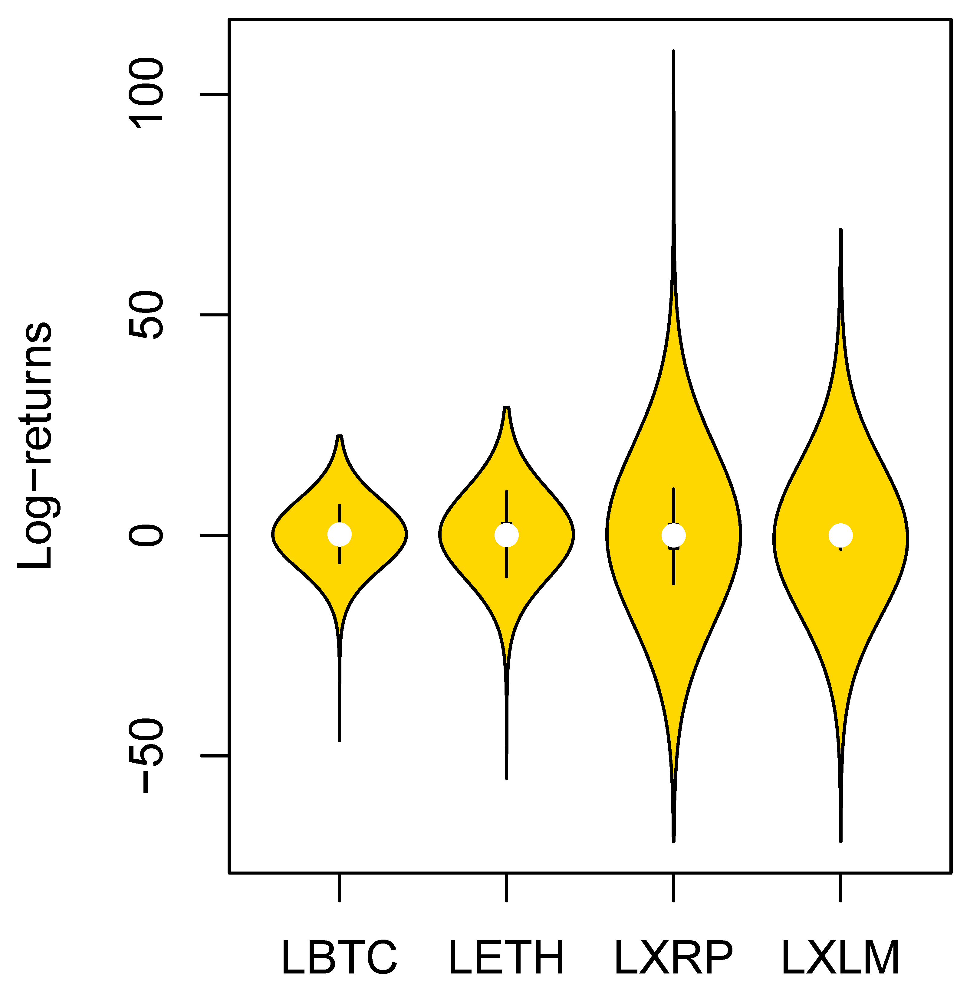
Using the four uniform datasets, we computed the directional dependence among the log returns using both copula and nonparametric methods. Figure 3 compares the violin plot pattern of the log returns of prices of BTC, ETH, XRP, and XLM (LBTC, LETH, LXRP, LXLM). As expected, LBTC had the smallest spread compared to the log returns of the three other cryptocurrencies (LETH, LXRP, LXLM), but LXLM had the largest spread compared to the log returns of the other three cryptocurrencies (LBTC, LETH, LXRP). Table 3 summarizes the descriptive statistics of the log return data of the cryptocurrencies such as the mean, skewness, and kurtosis as well as the maximum, minimum, range, standard deviation, and variance. Table 3 shows the average log return of ETH was the highest among the four cryptocurrencies. In Table 3, it is recognized that the standard deviation of LBTC was smaller than the other remaining cryptocurrencies, which means that LBTC had a smaller risk than the other cryptocurrencies in terms of investment. Moreover, the values of the kurtosis for the four cryptocurrencies were greater than three, meaning heavy tails compared to a normal distribution. LBTC and LETH were left-skewed while LXRP and LXLM were right-skewed. This meant that the log returns of Bitcoin and Ethereum were more likely to decrease soon whereas the log returns of Ripple and Stellar were more likely to increase. Table 4 shows the directional dependence (DD) computed from the nonparametric and copula methods. We noticed the DD difference between the two methods. Using the nonparametric DD method, we found that the DD from LBTC to LETH was slightly higher than the DD from LETH to LBTC, but with the copula DD method, we found that the DD from LBTC to LETH was slightly lower than the DD from LETH to LBTC. In terms of market cap, BTC was two times bigger than ETH. In terms of the long-term period viewpoint, it makes sense that the log returns of other altcoins and stablecoins are more influenced by LBTC rather than the other directional case. In light of these facts, the nonparametric DD method performed better than the copula DD method proposed by [15].

5. Conclusions

In this paper, we proposed an improved directional dependence by using a nonparametric method to rectify the issues of copula directional dependence used by [15]. Even though the computation time for our proposed method was longer than the current method, our proposed directional dependence did not require any assumptions and improved the accuracy of the proposed estimator in terms of root-mean-square error. Based on only two exemplifications, we also showed the performance of the nonparametric directional dependence method was superior to the copula directional dependence method with both simulated data and real data. In fact, the superiority of the nonparametric directional dependence method was not general in this paper. Thus, we need to consider the detailed general cases of the nonparametric directional dependence method in future studies. Our nonparametric directional dependence method will be useful in many research areas such as bioinformatics, economics, engineering, finance, geology, and neuroscience to see the directional dependence among many variables. In an era of big and complex data, our nonparametric directional dependence can be a good solution to reduce the level of uncertainty, which has been an issue in our society.

Author Contributions

Conceptualization, J.-M.K. and H.N.; methodology, J.-M.K. and H.N.; software, H.J. and H.N.; validation, J.-M.K., K.H.K. and H.N.; formal analysis, H.J., J.-M.K. and H.N.; investigation, J.-M.K., K.H.K. and H.N.; resources, H.N.; data curation, J.-M.K. and H.N.; writing original draft preparation, J.-M.K. and H.N.; writing review and editing, H.J., J.-M.K. and H.N.; visualization, J.-M.K. and H.N.; supervision, H.N.; project administration, J.-M.K. All authors have read and agreed to the published version of the manuscript.

Funding

This research was funded by the National Research Foundation of Korea funded by the Ministry of Education (NRF-2017R1D1A1A09000804).

Institutional Review Board Statement

Not applicable.

Informed Consent Statement

Not applicable.

Data Availability Statement

Not applicable.

Acknowledgments

The authors would like to thank the editor and the three anonymous respected referees for their suggestions, which have greatly improved the paper.

Conflicts of Interest

The authors declare no conflict of interest.

References

  1. Kim, J.-M.; Kim, S.; Kim, S.T. On the Relationship of Cryptocurrency Price with US Stock and Gold Price using Copula Models. Mathematics 2020, 8, 1859. [Google Scholar] [CrossRef]
  2. Sklar, M. Fonctions de repartition an dimensions et leurs marges. Publ. Inst. Statist. Univ. Paris 1959, 8, 229–231. [Google Scholar]
  3. Joe, H. Families of m-variate distributions with given margins and m (m − 1)/2 bivariate dependence parameters. In Distributions with Fixed Marginals and Related Topics; Rüschendorf, L., Schweizer, B., Taylor, M.D., Eds.; Institute of Mathematical Statistics: Washington, DC, USA, 1996; pp. 120–141. [Google Scholar]
  4. Bedford, T.; Cooke, R.M. Vines—A new graphical model for dependent random variables. Ann. Stat. 2002, 30, 1031–1068. [Google Scholar] [CrossRef]
  5. Aas, K.; Berg, D. Models for construction of multivariate dependence: A comparison study. Eur. Financ. 2009, 15, 639–659. [Google Scholar] [CrossRef]
  6. Aas, K.; Czado, C.; Frigessi, A.; Bakken, H. Pair-copula constructions of multiple dependence. Insur. Math. Econ. 2009, 44, 182–198. [Google Scholar] [CrossRef] [Green Version]
  7. Kurowicka, D.; Cooke, R.M. Distribution—Free continuous bayesian belief nets. In Proceedings of the Fourth International Conference on Mathematical Methods in Reliability Methodology and Practice, Santa Fe, NM, USA, 21–25 June 2004. [Google Scholar]
  8. Bauer, A.; Czado, C.; Klein, T. Pair-copula constructions for non-Gaussian DAG models. Can. J. Stat. 2012, 40, 86–109. [Google Scholar] [CrossRef] [Green Version]
  9. Brechmann, E.; Czado, C.; Aas, K. Truncated and simplified regular vines in high dimensions with application to financial data. Can. J. Stat. 2012, 40, 68–85. [Google Scholar] [CrossRef]
  10. Hobæk Haff, I.; Aas, K.; Frigessi, A. On the simplified pair-copula construction—Simply useful or too simplistic? J. Multivar. Anal. 2010, 101, 1296–1310. [Google Scholar] [CrossRef] [Green Version]
  11. Panagiotelis, A.; Czado, C.; Joe, H. Pair Copula Constructions for Multivariate Discrete Data. J. Am. Stat. Assoc. 2012, 107, 1063–1072. [Google Scholar] [CrossRef]
  12. Smith, M.; Min, A.; Almeida, C.; Czado, C. Modelling longitudinal data using a pair-copula decomposition of serial dependence. J. Am. Stat. 2010, 105, 1467–1479. [Google Scholar] [CrossRef]
  13. Masarotto, G.; Varin, C. Gaussian copula marginal regression. Electron. J. Stat. 2012, 6, 1517–1549. [Google Scholar] [CrossRef]
  14. Guolo, A.; Varin, C. Beta regression for time series analysis of bounded data, with application to Canada Google flu trends. Ann. Appl. Stat. 2014, 8, 74–88. [Google Scholar] [CrossRef]
  15. Kim, J.-M.; Hwang, S.Y. Directional dependence via gaussian copula beta regression model with asymmetric garch marginals. Commun. Stat. Simul. Comput. 2017, 46, 7639–7653. [Google Scholar] [CrossRef]
  16. Kim, J.-M.; Hwang, S.Y. The Copula Directional Dependence by Stochastic Volatility Models. Commun. Stat. Simul. Comput. 2019, 48, 1153–1175. [Google Scholar] [CrossRef]
  17. Hyun, S.; Lee, J.; Kim, J.M.; Jun, C. What Coins lead in the Cryptocurrency Market? Using Copula and Neural Networks Model. J. Risk Fin. Manag. 2019, 12, 132. [Google Scholar] [CrossRef] [Green Version]
  18. Sungur, E.A. Some observations on copula regression functions. Commun. Stat. Theory Methods 2005, 34, 1967–1978. [Google Scholar] [CrossRef]
  19. Doksum, K.; Samarov, A. Nonparametric Estimation of Global Functionals and a Measure of the Explanatory Power of Covariates in Regression. Ann. Stat. 1995, 23, 1443–1473. [Google Scholar] [CrossRef]
  20. Ferrari, S.; Cribari-Neto, F. Beta regression for modelling rates and proportions. J. Appl. Stat. 2004, 31, 799–815. [Google Scholar] [CrossRef]
  21. Fan, J.; Gijbels, I. Local Polynomial Modelling and Its Applications; Chapman & Hall: London, UK, 1996. [Google Scholar]
  22. Durante, F. Construction of non-exchangeable bivariate distribution functions. Stat. Pap. 2009, 50, 383–391. [Google Scholar] [CrossRef]
  23. Scarsini, M.; Venetoulias, A. Bivariate distributions with nonmonotone dependence structure. J. Am. Stat. Assoc. 1993, 88, 338–344. [Google Scholar]
Figure 1. Regression functions between the transformed variables with their best approximations (dotted line) under the first scenario.
Axioms 12 00293 g001
Figure 2. Regression functions between the transformed variables with their best approximations (dotted line) under the second scenario.
Axioms 12 00293 g002
Figure 3. Log return violin plots of LBTC, LETH, LXRP, and LXLM.
Axioms 12 00293 g003
Table 1. Root-mean-square error of the two estimators under the first scenario.
Sample Size U V V U
Nonparametric DDCopula DDNonparametric DDCopula DD
n = 1000.0770.0830.0760.056
n = 2000.0500.0760.0500.042
n = 4000.0350.0720.0330.031
n = 8000.0250.0710.0230.025
n = 16000.0180.0690.0160.021
Table 2. Root-mean-square error of the two estimators under the second scenario.
Sample Size U V V U
Nonparametric DDCopula DDNonparametric DDCopula DD
n = 100 0.0720.2080.0760.034
n = 200 0.0520.2120.0400.022
n = 400 0.0380.2130.0250.017
n = 800 0.0280.2140.0150.011
n = 1600 0.0210.2140.0100.008
Table 3. Summary Statistics of Log Returns (LBTC, LETH, LXRP, and LXLM).
LBTCLETHLXRPLXLM
Mean0.2130.2770.2420.260
Standard Deviation4.1335.6617.8969.118
Sample variance17.08032.04662.34283.145
Kurtosis11.8858.67434.17716.897
Skewness−0.797−0.4182.1351.133
Range68.98584.084179.176138.629
Minimum−46.473−55.071−69.315−69.315
Maximum22.51229.013109.86169.315
Sum387.253503.490439.491472.758
Count1817181718171817
Table 4. Directional dependence (DD) computed from the nonparametric and copula methods (the direction is from the row to the column).
Nonparametric DD Method
CoinLBTCLETHLXRPLXLM
LBTC 0.450.260.18
LETH0.44 0.360.21
LXRP0.260.35 0.26
LXLM0.180.230.27
Copula DD Method
CoinLBTCLETHLXRPLXLM
LBTC 0.390.210.14
LETH0.4 0.290.18
LXRP0.220.3 0.23
LXLM0.140.170.21
Disclaimer/Publisher’s Note: The statements, opinions and data contained in all publications are solely those of the individual author(s) and contributor(s) and not of MDPI and/or the editor(s). MDPI and/or the editor(s) disclaim responsibility for any injury to people or property resulting from any ideas, methods, instructions or products referred to in the content.