Article

A Fractional Rheological Model of Viscoanelastic Media

by
Armando Ciancio
1,
Vincenzo Ciancio
2 and
Bruno Felice Filippo Flora
3,*
1
Department of Biomedical and Dental Sciences and Morphofunctional Imaging (BIOMORF), University of Messina, Via Consolare Valeria c/o A.O.U. Policlinico ’G.Martino’, 98126 Messina, Italy
2
Accademia Peloritana dei Pericolanti, Piazza S. Pugliatti 1, 98122 Messina, Italy
3
Azienda Ospedaliera “Papardo”, Viale F. Stagno d’Alcontres 34, 98158 Messina, Italy
*
Author to whom correspondence should be addressed.
Axioms 2023, 12(3), 243; https://doi.org/10.3390/axioms12030243
Submission received: 22 December 2022 / Revised: 20 February 2023 / Accepted: 24 February 2023 / Published: 27 February 2023
(This article belongs to the Special Issue Special Topics in Differential Equations with Applications)

Abstract

:
The mechanical behaviour of materials can be described by a phenomenological relationship that binds strain to stress, by the complex modulus function: M ( ω ) , which represents the frequency response of the medium in which a transverse mechanical wave is propagated. From the experimental measurements of the internal friction obtained when varying the frequency of a transverse mechanical wave, the parameters that characterize the complex module are determined. The internal friction or loss tangent is bound to the dissipation of the specific mechanical energy. The non-equilibrium thermodynamics theory leads to a general description of irreversible phenomena such as relaxation and viscosity that can coexist in a material. Through the state variables introduced by Ciancio and Kluitenberg, and applying the fractional calculation due to a particular memory mechanism, a model of a viscoanelastic medium is obtained in good agreement with the experimental results.

1. Introduction

In the second half of the 20th century, a theory was proposed for the study of mechanical [1,2,3,4,5,6,7,8,9,10,11,12,13,14,15,16] and electromagnetic [17,18,19,20,21] phenomena in continuous media which is based on the general methods of non-equilibrium thermodynamics. In the hypothesis that different microscopic phenomena produce inelastic strains (instance slip, dislocation) and effects similar to the flow of ordinary viscous fluids, the entropy is characterized by internal energy and inelastic strain tensors; then the expression of entropy production obtained characterizes the state of non-equilibrium. Zener conducted experimental investigations on the mechanical behaviour of solids subject to the action of given stress [22]. In particular, by carrying out measurements of internal friction they were able to describe the process of relaxation due to the anelasticity media. The proposed anelastic media were only valid for some frequency values. Many years later, Caputo and Mainardi proposed a model of viscoanelastic media using Caputo’s fractional derivative [23,24]. This is an integral operator whose kernel represents the memory effect. Viscoelastic media have been studied in the field of finite strains by Coleman and Noll [25,26]. An extension of the many viscoelastic models to the fractional calculation have been resumed as in [27]. In the case of elastic and viscoelastic means this effect is evanescent [28]. The Caputo–Mainardi model is very different at low frequencies from the experimental values. Concurrently with the study of systems with memory, fractional calculus theory has been developed and has been used in several applications, allowing a greater physical understanding of the problems. In particular, the use of local fractional derivatives [29,30,31,32,33,34] has made it possible to obtain models in good agreement with the experimental data highlighting, in relation to the physical problem studied, the dependence of the order of local fractional derivation from the processes of relaxation in the media with memory. To obtain a mechanical representation consistent with the description of the relaxation processes valid for many solid viscoanelastic materials and over a wide range of frequencies, in Section 2, from thermodynamic considerations of non-reversible processes synthesized in the definition of specific entropy and total strain tensor for small field displacements, the rheological equation is derived. The rheological equation allows the stress tensor to be determined by means of internal variables and phenomenological coefficients, when the strain tensor resulting from the displacement field and the rheological coefficients are known, the latter obtained by experimental measurements. In Section 3, from the rheological equation relating to viscoanelastic media, passing into the Laplace transform domain, a mechanical representation with four parameters is obtained, where the components of the model, responsible for the relaxation process, are characterized through two relaxation times, one due to the viscosity understood in solids as slipping of crystalline planes and the other due to the inelasticity. To evaluate the memory effect, we consider relaxation times expressible by means of real exponentials. For this purpose, in Section 4, in the rheological equation we use the Caputo fractional derivative to obtain a four-parameter fractional model. As pointed out by Berry, impurities and defects in the crystal lattice cause more relaxation processes independent of each other. In Section 5, the fractional model is extended to two relaxation processes, resulting in an eight-parameter model. Using the Zener experimental curves in tabular form, in Section 6, we show the results obtained for aluminium, brass and steel in relation to the eight-parameter model by applying the differential evolution (DE) algorithm. Unlike other works on viscoelastic media [35], we have taken into consideration the DE algorithm to determine the parameters of the fractional model of viscoanelastic media, the latter consistent with the principles of thermodynamics.

2. The Rheological Equation

If both elastic and inelastic deformations occur, for index α , β 1 , 2 , 3 , we have:
ϵ α β = ϵ α β ( 0 ) + ϵ α β ( 1 )
where ϵ α β is the tensor of total strain and ϵ α β ( 0 ) and ϵ α β ( 1 ) are tensors describing the elastic and inelastic strain, respectively. Therefore the entropy will depend on the internal energy u, on the ϵ α β . Hence [5,6,7]:
s = s u , ϵ α β , ϵ α β ( 1 )
where s is specific entropy and u is internal energy. The temperature is:
T 1 = u s u , ϵ α β , ϵ α β ( 1 )
and we define the equilibrium-stress tensor:
τ α β ( e q ) = ρ T ϵ α β s u , ϵ α β , ϵ α β ( 1 )
and
τ α β ( 1 ) = ρ T ϵ α β ( 1 ) s u , ϵ α β , ϵ α β ( 1 )
where ρ is the mass density and we will call τ α β ( 1 ) the affinity stress tensor conjugate to ϵ α β ( 1 ) .
By using Equations (3)–(5) from (1) we obtain the differential d s of s :
T d s = d u ν τ α β ( e q ) d ϵ α β + ν τ α β ( 1 ) d ϵ α β ( 1 )
where ν = ρ 1 is the specific volume (volume for unit of mass). Relation (6) is called the Gibbs relation in which the usual summation convention for the dummy index is used. In the following we will use the deviator A ˜ α β of an arbitrary tensor field A α β , ie:
A ˜ α β = A α β A
where
A = 1 3 A α α = 1 3 A 11 + A 22 + A 33
and the specific free energy f:
f = u T s
From (3) and (6) we have:
d f = s d T + ν τ α β ( e q ) d ϵ α β ν τ α β ( 1 ) d ϵ α β ( 1 )
and, hence:
τ α β ( e q ) = ρ ϵ α β f u , ϵ α β , ϵ α β ( 1 )
τ α β ( 1 ) = ρ ϵ α β ( 1 ) f u , ϵ α β , ϵ α β ( 1 )
Assuming that the strains are small from a geometrical point of view:
ϵ α β = 1 2 u α x β + u β x α
where u α are the components of the displacement field and the stress tensors τ α β ( e q ) and τ α β ( 1 ) are linear functions of the strain tensors and of temperature; we suppose that f has the form [6,7]:
f = ν 0 · f ( a ) ϵ ˜ α β , ϵ α β , ϵ α β ( 1 ) + f ( b ) ϵ ˜ α β , ϵ α β , ϵ α β ( 1 ) + 3 T T 0 c ( 0 ) ϵ α β c ( 1 ) ϵ α β ( 1 ) ψ ( T )
where
f ( a ) ϵ ˜ α β , ϵ α β , ϵ α β ( 1 ) = 1 2 a ( 0 , 0 ) ϵ ˜ α β ϵ ˜ α β 2 ϵ α β ( 1 ) + 1 2 a ( 1 , 1 ) ϵ ˜ α β ( 1 ) 2
f ( b ) ϵ ˜ α β , ϵ α β , ϵ α β ( 1 ) = 1 2 b ( 0 , 0 ) ϵ α β ϵ α β 2 ϵ α β ( 1 ) + 3 2 b ( 1 , 1 ) ϵ α β ( 1 ) 2
In (14) the strain is measured with respect to a reference state, ν 0 is specific volume, T 0 is the temperature of the media in the reference state and a ( 0 , 0 ) , a ( 1 , 1 ) , b ( 0 , 0 ) , b ( 1 , 1 ) , c ( 0 ) , c ( 1 ) are scalar constants [6,7,8,9]. Finally, ψ ( T ) is same function of the temperature. Using (11) and (12) from (14) one obtains the following expression for the deviators of tensors τ ˜ α β ( e q ) and τ ˜ α β ( 1 ) :
τ ˜ α β ( e q ) = a ( 0 , 0 ) ϵ ˜ α β ( 0 )
τ ˜ α β ( e q ) = a ( 0 , 0 ) ϵ ˜ α β a ( 1 , 1 ) ϵ ˜ α β ( 1 )
Making τ ˜ α β the mechanical stress tensor which occurs in the equation of motion and in the first law of thermodynamics, the viscous stress tensor τ ˜ α β ( v i ) is defined by:
τ α β ( v i ) = τ α β τ α β ( e q )
Furthermore, we introduce [9] the following flow laws for slicer phenomena in isotropic media:
d d t ϵ ˜ α β ( 1 ) = η s ( 1 , 1 ) τ ˜ α β ( 1 ) + η s ( 1 , 0 ) d d t ϵ ˜ α β
τ α β ( v i ) = η s ( 0 , 1 ) τ ˜ α β ( 1 ) + η s ( 0 , 0 ) d d t ϵ ˜ α β
The scalar η s ( i , j ) ( i , j = 0 , 1 ) are called phenomenological coefficients. Using (2) and (19) one may eliminate ϵ ˜ α β ( 0 ) , ϵ ˜ α β ( 1 ) , τ ˜ α β ( e q ) , τ ˜ α β ( 1 ) , and τ ˜ α β ( v i ) , from the Equations of state (17) and (18) and the phenomenological Equations (20) and (21) one has:
R ( d ) 0 ( τ ) τ ˜ α β + d d t τ ˜ α β = R ( d ) 0 ( ϵ ) ϵ ˜ α β + R ( d ) 1 ( ϵ ) d d t ϵ ˜ α β + R ( d ) 2 ( ϵ ) d 2 d t 2 ϵ ˜ α β
where
R ( d ) 0 ( ϵ ) = a ( 1 , 1 ) η s ( 1 , 1 )
R ( d ) 0 ( ϵ ) = a ( 0 , 0 ) a ( 1 , 1 ) a ( 0 , 0 ) η s ( 1 , 1 )
R ( d ) 1 ( ϵ ) = a ( 0 , 0 ) 1 + 2 η s ( 0 , 1 ) + a ( 1 , 1 ) η s ( 0 , 0 ) η s ( 1 , 1 ) + η s ( 0 , 1 ) 2
R ( d ) 2 ( ϵ ) = η s ( 0 , 0 )

3. Mechanical Representation of the Viscoanelastic Media According to the Ciancio–Kluitenberg Model

Several mechanical representations of the media have been given regarding the binding between stress and deformation [29]. In this section, we apply the Ciancio–Kluitenberg theory to the problem of determining the deformation to which a viscoanelastic medium is subject under the action of a stress. Subsequently we provide a mechanical representation of the viscoanelastic medium in a Laplace domain. For elastic materials, the binding between the strain deviator tensor ϵ ˜ α β and the stress one τ ˜ α β is of the type:
ϵ ˜ α β ( k , ω ) = M 0 τ ˜ α β ( k , ω )
where Equation (27) represents the equivalent Hooke’s law and M 0 1 = c o s t . t e is the elastic constant that depends on the material and is a real number. In the case of anelastic, viscoelastic, and viscoanelastic material, the constitutive binding between the strain deviator tensor ϵ ˜ α β and the stress tensor τ ˜ α β is of the type:
ϵ ˜ α β ( k , ω ) = ( M ( ω ) M 0 ) τ ˜ α β ( k , ω )
where M ( ω ) is the complex modulus, while M ˜ ( ω ) = M ( ω ) M 0 is the non-elastic component of the complex modulus at the ω angular frequency produced by the displacement field u α with α = 1 , 2 , 3 :
ϵ α β = ϵ ˜ α β = 1 2 x β u α + x α u β
Considering small displacements, the substantial derivative coincides with the local one:
d d t = t
The rheological equation of a viscoanelastic medium for Equation (22) becomes:
R ( d ) 0 ( τ ) τ ˜ α β + t τ ˜ α β = R ( d ) 0 ( ϵ ) ϵ ˜ α β + R ( d ) 1 ( ϵ ) t ϵ ˜ α β + R ( d ) 2 ( ϵ ) t t 2 ϵ ˜ α β
where the parameters R ( d ) 0 ( τ ) , R ( d ) 0 ( ϵ ) , R ( d ) 1 ( ϵ ) , and R ( d ) 2 ( ϵ ) are the reological coefficients. Therefore the Ciancio–Kluitenberg model characterizes a single relaxation process with four parameters, i.e., the four rheological coefficients.
Transforming both members of Equation (30) according to Laplace we obtain:
R ( d ) 0 ( τ ) τ ˜ α β * + s τ ˜ α β * = R ( d ) 0 ( ϵ ) ϵ ˜ α β * + s R ( d ) 1 ( ϵ ) ϵ ˜ α β * + s 2 R ( d ) 2 ( ϵ ) ϵ ˜ α β *
where
τ ˜ α β * = 0 τ ˜ α β e s t d t
ϵ ˜ α β * = 0 ϵ ˜ α β e s t d t
rearranging the terms present in the Equation (31), we obtain
ϵ ˜ α β * ( s ) = R ( d ) 0 ( τ ) + s R ( d ) 0 ( ϵ ) + s R ( d ) 1 ( ϵ ) + s 2 R ( d ) 2 ( ϵ ) τ ˜ α β * ( s )
that we rewrite as:
ϵ ˜ α β * ( s ) = R ( d ) 0 ( τ ) R ( d ) 0 ( ϵ ) 1 + s 1 R ( d ) 0 ( τ ) 1 + s R ( d ) 1 ( ϵ ) R ( d ) 0 ( ϵ ) + s 2 R ( d ) 2 ( ϵ ) R ( d ) 0 ( ϵ ) τ ˜ α β * ( s )
It is observed that by placing:
t 1 = 1 R ( d ) 0 ( τ )
t 2 = M 0 R ( d ) 0 ( ϵ )
M 0 = R ( d ) 1 ( ϵ ) 1
ω 0 2 = M 0 t 2 R ( d ) 2 ( ϵ )
Equation (35) becomes:
ϵ ˜ α β * ( s ) = M 0 t 2 t 1 1 + t 1 s 1 + t 2 s + s ω 0 2 τ ˜ α β * ( s )
From the comparison with Equation (28), we obtain:
M ( ω ) = M 0 1 + t 2 t 1 1 + t 1 s 1 + t 2 s + s ω 0 2
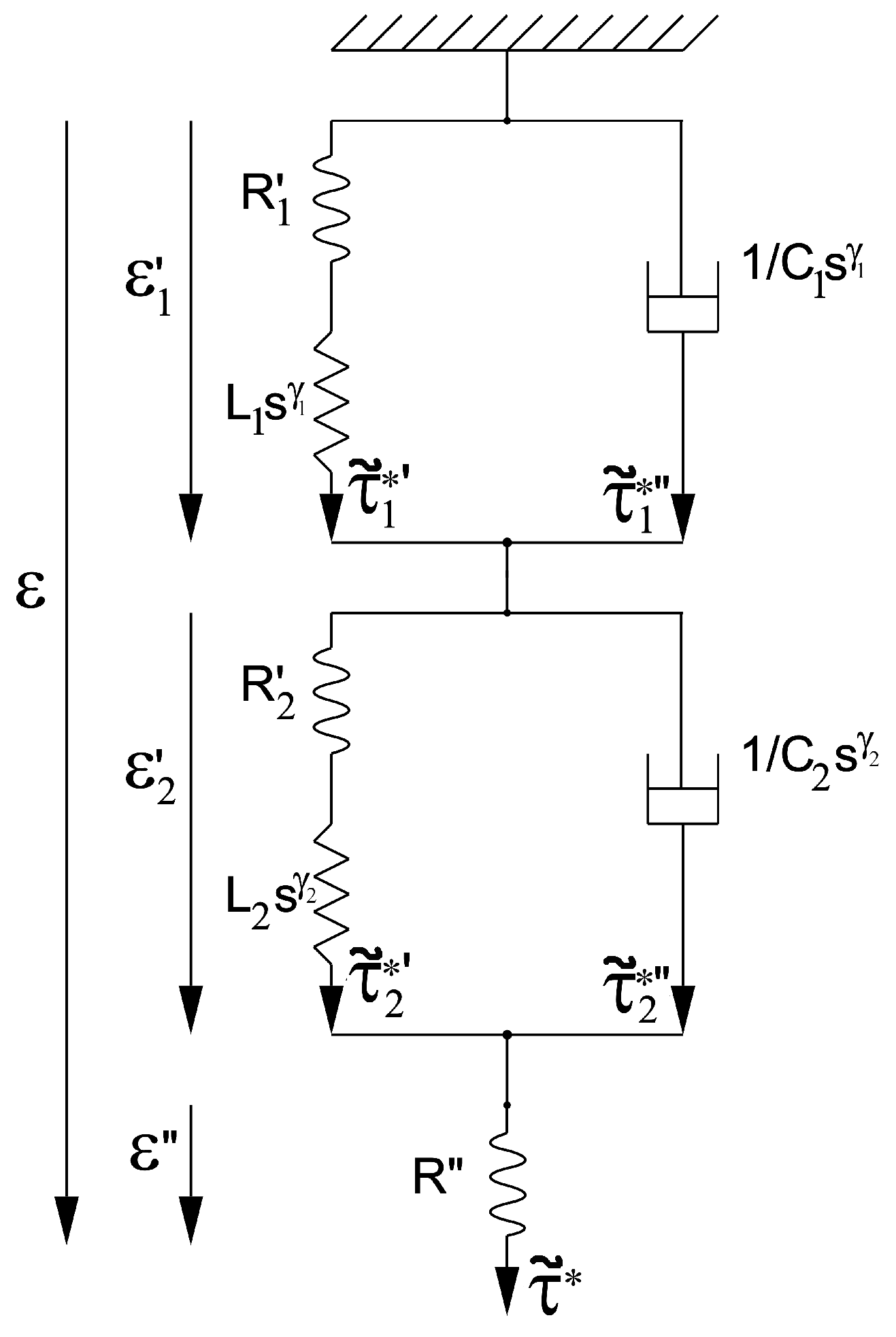
Figure 1 shows the mechanical representation of viscoanelastic media in the Laplace domain. Here, we observe how the spring, compliance, and resistance have the electrical equivalent of resistance, capacitance, and inductance, respectively. R and R represent the parameters that characterize the elastic component of the medium, indicated with the spring symbol, C represents the compliance denoted by means of the vibration damper, and L represents the resistance that opposes the medium to deformation. All parameters are constant: t 1 = L R , t 2 = R C , ω 0 = 1 L C , M 0 = R and M 0 t 2 t 1 = R where ϵ ˜ α β * ( s ) = ε = ε + ε and τ ˜ α β * ( s ) = τ ˜ * = τ ˜ * + τ ˜ * . If L = 0 and R = 0 then the mechanical representation coincides with that of a viscoelastic medium, where the viscosity part is given by compliance C and the elastic part is given by R . Hence the anelastic part is characterized by branch R + L s , whereas the viscosity part is characterized by branch 1 / C s .

4. Fractional Rheological Model with Four Parameters of a Viscoanelastic Medium for a Single Relaxation Process

It is experimentally verifiable that, with the passage of time, the elastic or viscoelastic material tends to forget its more remote history; that is the deformations to which it has been subjected in the past tend to have less and less influence on the current deformation [28]. In viscoanelastic media the memory effect is permanent. From a mathematical point of view, this implies that relaxation time is a power of fractional order. It is preferred not to proceed with the dimensionless method, as in [36], to highlight that relaxation time is a real power of fractional order. From Ciancio–Kluitenberg’s theory and fractional calculation, we obtain the following rheological equation:
R ( d ) 0 ( τ ) τ ˜ α β + t γ τ ˜ α β = R ( d ) 0 ( ϵ ) ϵ ˜ α β + R ( d ) 1 ( ϵ ) t γ ϵ ˜ α β + R ( d ) 2 ( ϵ ) t t 2 γ ϵ ˜ α β
where t γ · is fractional derivative of order γ with respect to time and 0 < γ 1 . From a physical point of view it is natural to apply the fractional derivative of Caputo [23] that characterizes the means with memory in which the relaxation process is observed:
C t γ f ( x , t ) = 1 Γ ( 1 γ ) 0 t w f ( x , w ) ( t w ) γ d w
Applying the Fourier transform to the rheological Equation (42), we obtain:
ε ˜ α β k , ω = M 0 t 2 t 1 1 + t 1 ( i ω ) γ 1 + t 2 ( i ω ) γ + ( i ω / ω 0 ) 2 γ τ ˜ α β k , ω
From comparison with the constitutive Equation (28), the complex module is obtained:
M ( ω ) = M 0 1 + t 2 t 1 1 + t 1 ( i ω ) γ 1 + t 2 ( i ω ) γ + ( i ω / ω 0 ) 2 γ
Identification of rheological parameters:
  • R ( d ) 0 ( τ ) = 1 t 1 , depends on the stress time constant t 1 , with:
    t 1 = ( t 1 / 2 π ) γ
  • R ( d ) 0 ( ϵ ) = M 0 t 2 , depends on the stress relaxation time t 2 , with:
    t 2 = ( t 2 / 2 π ) γ
  • R ( d ) 1 ( ϵ ) 1 = M 0 , coincides with the complex module due to the impulsive stress applied at the initial instant.
  • R ( d ) 2 ( ϵ ) = M 0 t 2 ω 0 2 γ , depends on natural angular frequency ω 0
We observe how the rheological coefficients depend on the characteristic parameters, i.e., by relaxation time due to the stress and deformation, respectively, and natural angular frequency. Determining the parameters experimentally it will therefore be possible to obtain the values of state variables.

5. Fractional Rheological Model with Eight Parameters of a Viscoanelastic Medium for Two Single Relaxation Processes

Although the behaviour of viscoanelastic media can be described using models developed by Zener [37] and other authors such as Caputo and Mainardi [24], they present a significant discrepancy with experimental values of internal friction (IF) [38,39,40]. This discrepancy can be reduced by considering the presence of several independent relaxation processes that also take into account the impurity of materials at the microscopic level due to the presence of defects in the crystalline lattice or different atomic configuration characteristics of other materials. It is natural to think of an extension of the theory by applying the principle of superposition to n relaxation processes [40]. Applying the principle of superposition in the case of n relaxation processes, we obtain:
M ( ω ) M 0 = 1 + q = 1 m t 2 , q t 1 , q 1 + t 1 , q ( i ω ) γ q 1 + t 2 , q ( i ω ) γ q + ( i ω / ω 0 , q ) 2 γ q
a model with 4 m parameters. For m = 2 , i.e., with two relaxation processes, we obtain a rheological model with eight parameters (Figure 2):
p = t 1 , 1 , t 2 , 1 , γ 1 , ω 0 , 1 , t 1 , 2 , t 2 , 2 , γ 2 , ω 0 , 2
where t 11 = L 1 R 1 , t 21 = R 1 C 1 , ω 01 = 1 L 1 C 1 , M 0 t 21 t 11 = R 1 , t 12 = L 2 R 2 , t 22 = R 2 C 2 , ω 02 = 1 L 2 C 2 , M 0 t 22 t 12 = R 2 , M 0 = R
with ϵ ˜ α β * ( s ) = ε = ε 1 + ε 2 + ε and τ ˜ α β * ( s ) = τ ˜ * = τ ˜ 1 * + τ ˜ 1 * = τ ˜ 2 * + τ ˜ 2 * . The eight parameters, four for each of the two relaxation processes, bound to the corresponding rheological coefficients, are obtained by applying the differential evolution (DE) algorithm from experimental measurements of the so-called internal friction, IF( ω ), or loss tangent: I F ( ω ) = I m a g ( M ( ω ) ) R e a l ( M ( ω ) ) , relating to the dissipation of mechanical energy due to internal friction as the frequency changes. This function is given by the relationship between the imaginary and the real part of the complex module, which for small losses of the medium coincides with the specific dissipation function.

6. Numerical Results

In this section, we simulate the eight-parameter fractional model considering the experimental data [38]. The IF experimental data are given in the figure on page 55 of [37] and from this are appropriately extracted and shown in Table 1, corresponding to certain frequency values and relative to the metals: steel, brass, and aluminium.
To this end we use the differential evolution (DE) algorithm [41] that minimizes the objective function J ( p ) for determining the parameters p = t 1 , 1 , t 2 , 1 , γ 1 , ω 0 , 1 , t 1 , 2 , t 2 , 2 , γ 2 , ω 0 , 2 of the model. The DE algorithm [42] is an iterative method of a stochastic nature for the search for the possible optimal solutions on a large space of the parameters. In this work, it has been used in the Python language with the use of the scipy library [43,44]. The DE was chosen for its ability to provide optimal possible solutions without resorting to classical methods of finding solutions such as the gradient method or Newton’s method with which it is easy to fall into local minimums, where use requires differentiation of functions. The objective function J ( p ) taken into account is the mean square relative error between the experimental values of the internal friction I F ^ ( f i ) and the values related to the eight-parameter fractional model I F ( f i ) at frequencies f i , i = 1 , 2 , . . . , m :
J ( p ) = 1 m + 1 i = 1 m I F ^ ( f i ) I F ( f i ; p ) I F ^ ( f i ) 2
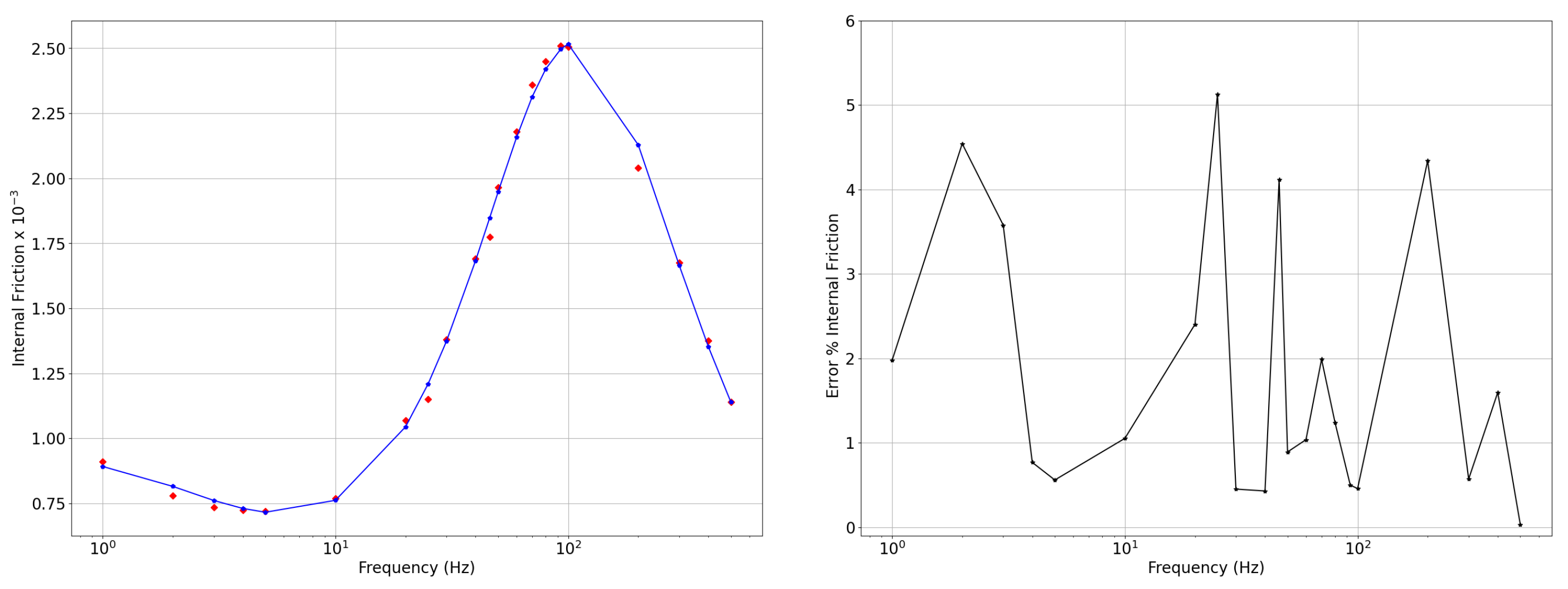
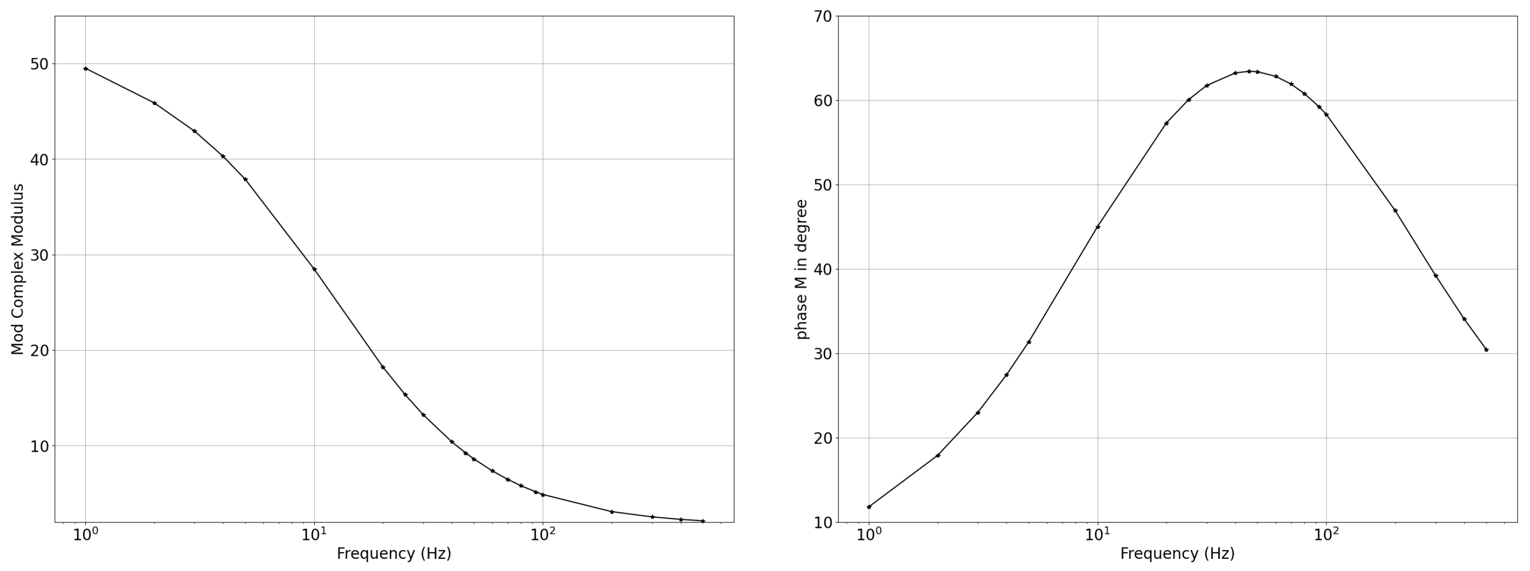
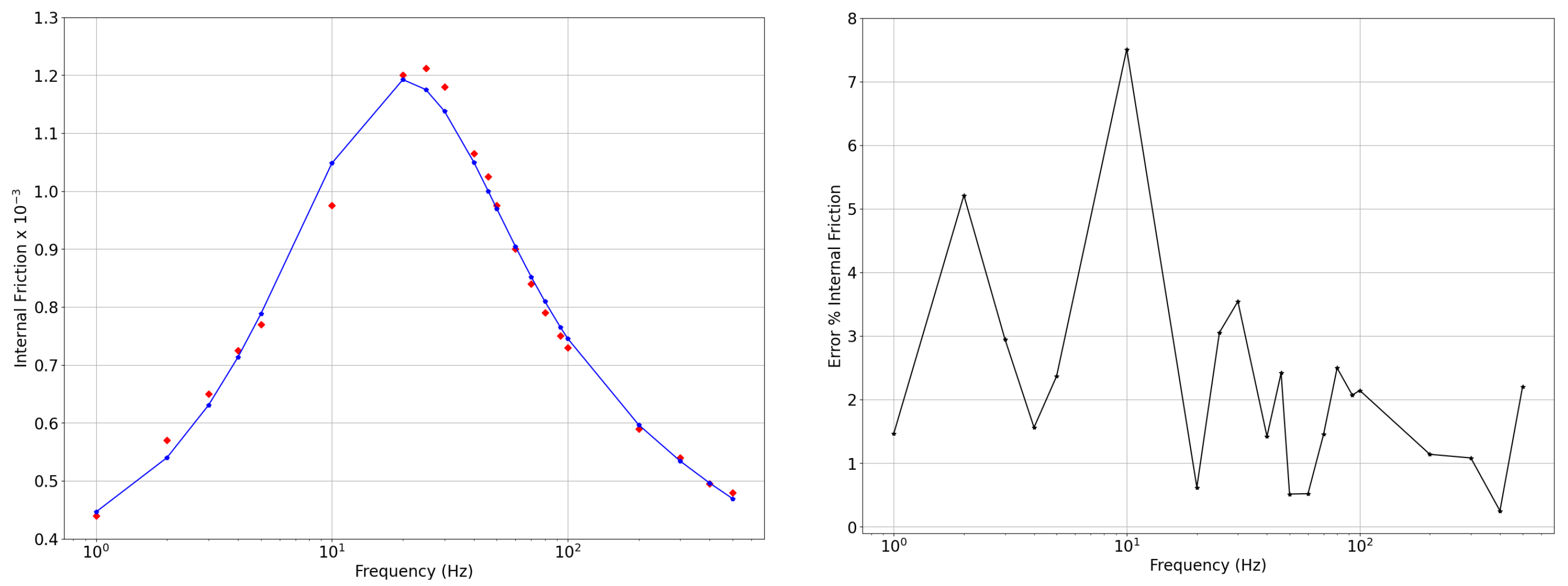
In Table 2 and Table 3, we obtain the model parameters and the rheological coefficients of the aluminium, respectively. In Figure 3, to the variation of the frequency, it is brought back in the panel of left the shape of the internal friction while in the one of right the relative percentage error for aluminium. In Figure 4, it is brought back in the panel of left the real part while in the one right the imaginary part of the modulus complex for aluminium. In Table 4 and Table 5, we obtain the model parameters and the rheological coefficients of the brass, respectively. In Figure 5, to the variation of the frequency, it is brought back in the panel of left the shape of the internal friction while in the one of right the relative percentage error for brass. In Figure 6, it is brought back in the panel of left the real part while in the one right the imaginary part of the modulus complex for brass. Finally, in Table 6 and Table 7 we obtain the model parameters and the rheological coefficients of the steel, respectively. In Figure 7, to the variation of the frequency, it is brought back in the panel of left the shape of the internal friction while in the one of right the relative percentage error for steel. In Figure 8, it is brought back in the panel of left the real part while in the one right the imaginary part of the modulus complex for steel.

7. Conclusions

Applying the Ciancio–Kluitenberg theory, in this work a mechanical representation of a viscoanelastic medium has been found that allows the problem to be solved of determining the state of the system solicited by a stress. Unlike previous models, the mechanical representation found is consistent with the relaxation processes observed in relation to the type of material considered. Moreover, it is very general in that the case of viscoelastic media is obtained as a limit case of inelastic media. Using the DE algorithm, which minimizes the relative quadratic error in the calculation of internal friction (IF), the values of the eight parameters or eight rheological coefficients have been determined. The results obtained confirm the validity of the eight-parameter model whose relative percentage error does not exceed 5% over almost the entire frequency range. In addition, it was possible to obtain the trend of the complex module M (module and phase). In all metals it is observed that the fractional order is less than 1; this characteristic is typical in the propagation of mechanical waves at low frequency from 0 to 500 Hz. Finally, the values obtained of the rheological coefficients, for all the metals considered here, are positive in accordance with the second principle of thermodynamics.

Author Contributions

Conceptualization, A.C., V.C. and B.F.F.F.; methodology, A.C., V.C. and B.F.F.F.; software, B.F.F.F.; validation, A.C., V.C. and B.F.F.F.; formal analysis, A.C., V.C. and B.F.F.F.; data curation, A.C., V.C. and B.F.F.F.; writing—original draft preparation, B.F.F.F.; visualization, A.C., V.C. and B.F.F.F. All authors have read and agreed to the published version of the manuscript.

Funding

This research received no external funding.

Institutional Review Board Statement

Not applicable.

Informed Consent Statement

Not applicable.

Data Availability Statement

The data presented in this study are available in the article.

Conflicts of Interest

The authors declare no conflict of interest.

References

  1. Kluitenberg, G. On rheology and thermodynamics of irreversible processes. Physica 1962, 28, 1173–1183. [Google Scholar] [CrossRef]
  2. Kluitenberg, G. A note on the thermodynamics of Maxwell bodies, Kelvin bodies (Voigt bodies), and fluids. Physica 1962, 28, 561–568. [Google Scholar] [CrossRef]
  3. Kluitenberg, G. On the thermodynamics of viscosity and plasticity. Physica 1963, 29, 633–652. [Google Scholar] [CrossRef]
  4. Kluitenberg, G. On heat dissipation due to irreversible mechanical phenomena in continuous media. Physica 1967, 35, 177–192. [Google Scholar] [CrossRef]
  5. Kluitenberg, G. A thermodynamic derivation of the stress–strain relations for burgers media and related substances. Physica 1968, 38, 513–548. [Google Scholar] [CrossRef]
  6. Kluitenberg, G.; Ciancio, V. On linear dynamical equations of state for isotropic media I: General formalism. Phys. Stat. Mech. Appl. 1978, 93, 273–286. [Google Scholar] [CrossRef]
  7. Cianco, V.; Kluitenberg, G. On linear dynamical equations of state for isotropic media II. Phys. Stat. Mech. Appl. 1979, 99, 592–600. [Google Scholar] [CrossRef]
  8. Ciancio, V. Propagation and attenuation of singular wave surfaces in linear inelastic media. Phys. Stat. Mech. Appl. 1979, 97, 127–138. [Google Scholar] [CrossRef]
  9. Turrisi, E.; Ciancio, V.; Kluitenberg, G. On the propagation of linear transverse acoustic waves in isotropic media with mechanical relaxation phenomena due to viscosity and a tensorial internal variable II. Some cases of special interest (Poynting-Thomson, Jeffreys, Maxwell, Kelvin-Voigt, Hooke and Newton media). Phys. Stat. Mech. Appl. 1982, 116, 594–603. [Google Scholar] [CrossRef]
  10. Ciancio, V.; Bartolotta, A.; Farsaci, F. Experimental confirmations on a thermodynamical theory for viscoanelastic media with memory. Phys. Condens. Matter 2007, 394, 8–13. [Google Scholar] [CrossRef]
  11. Ciancio, A.; Ciancio, V.; Farsaci, F. Wave propagation in media obeying a thermoviscoanelastic model. UPB Sci. Bull. Ser. A 2007, 69, 69–79. [Google Scholar]
  12. Ciancio, V.; Ciancio, A.; Farsaci, F. On general properties of phenomenological and state coefficients for isotropic viscoanelastic media. Phys. Condens. Matter 2008, 403, 3221–3227. [Google Scholar] [CrossRef]
  13. Ciancio, A. An approximate evalutation of the phenomenological and state coefficients for viscoanelastic media with memory. U.P.B. Sci. Bull. 2011, 73, 3–14. [Google Scholar]
  14. Ciancio, V.; Restuccia, L. On heat equation in the framework of classic irreversible thermodynamics with internal variables. Int. J. Geom. Methods Mod. Phys. 2016, 13, 1640003. [Google Scholar] [CrossRef]
  15. Ciancio, V.; Palumbo, A. A thermodynamical theory with internal variables describing thermal effects in viscous fluids. J. -Non-Equilib. Thermodyn. 2018, 43, 171–184. [Google Scholar] [CrossRef]
  16. Ciancio, V. On the temperature equation in classical irreversible thermodinamics. Appl. Sci. 2022, 24, 71–86. [Google Scholar]
  17. Ciancio, V. On the Generalized Debye Equation for Media with Dielectric Relaxation Phenomena Described by Vectorial Internal Thermodynamic Variables. J. Non-Equilib. Thermodyn. 1989, 14, 239–250. [Google Scholar] [CrossRef]
  18. Ciancio, V.; Kluitenberg, G. On electromagnetic waves in isotropic media with dielectric relaxation. Acta Phys. Hung. 1989, 66, 251–276. [Google Scholar] [CrossRef]
  19. Ciancio, V.; Restuccia, L.; Kluitenberg, G. A Thermodynamic Derivation of Equations for Dielectric Relaxation Phenomena in Anisotropic Polarizable Media. J. Non.-Equil. Thermodyn. 1990, 15, 157–172. [Google Scholar] [CrossRef]
  20. Ciancio, V.; Farsaci, F.; Di Marco, G. A method for experimental evaluation of phenomenological coefficients in media with dielectric relaxation. Phys. Condens. Matter 2007, 387, 130–135. [Google Scholar] [CrossRef]
  21. Ciancio, V.; Verhás, J. A Thermodynamic Theory for Heat Radiation Through the Atmosphere. J. Non.-Equil. Thermodyn. 1991, 16, 57–66. [Google Scholar] [CrossRef]
  22. Zener, C. Internal friction in solids. Proc. Phys. Soc. 1940, 52, 152. [Google Scholar] [CrossRef]
  23. Caputo, M. Linear Models of Dissipation whose Q is almost Frequency Independent—II. Geophys. J. Int. 1967, 13, 529–539. [Google Scholar] [CrossRef]
  24. Caputo, M.; Mainardi, F. A new dissipation model based on memory mechanism. Pure Appl. Geophys. 1971, 91, 134–147. [Google Scholar] [CrossRef]
  25. Coleman, B.D.; Noll, W. The thermodynamics of elastic materials with heat conduction and viscosity. Arch. Ration. Mech. Anal. 1963, 13, 167–178. [Google Scholar] [CrossRef]
  26. Coleman, B.D.; Noll, W. Foundations of linear viscoelasticity. Rev. Mod. Phys. 1961, 33, 239. [Google Scholar] [CrossRef]
  27. Shen, L.J. Fractional derivative models for viscoelastic materials at finite deformations. Int. J. Solids Struct. 2020, 190, 226–237. [Google Scholar] [CrossRef]
  28. Fichera, G. Sul principio della memoria evanescente. Rend. Semin. Mat. Della Univ. Padova 1982, 68, 245–259. [Google Scholar]
  29. Mainardi, F.; Spada, G. Creep, relaxation and viscosity properties for basic fractional models in rheology. Eur. Phys. J. Spec. Top. 2011, 193, 133–160. [Google Scholar] [CrossRef] [Green Version]
  30. Ciancio, A.; Flora, B.F.F. A Fractional Complex Permittivity Model of Media with Dielectric Relaxation. Fractal Fract. 2017, 1, 4. [Google Scholar] [CrossRef] [Green Version]
  31. Ciancio, A.; Ciancio, V.; d’Onofrio, A.; Flora, B.F.F. A Fractional Model of Complex Permittivity of Conductor Media with Relaxation: Theory vs. Experiments. Fractal Fract. 2022, 6, 390. [Google Scholar] [CrossRef]
  32. Caputo, M.; Fabrizio, M. A new definition of fractional derivative without singular kernel. Prog. Fract. Differ. Appl. 2015, 1, 73–85. [Google Scholar]
  33. Tarasov, V.E.; Tarasova, S.S. Fractional derivatives and integrals: What are they needed for? Mathematics 2020, 8, 164. [Google Scholar] [CrossRef] [Green Version]
  34. Tarasov, V.E. No nonlocality. No fractional derivative. Commun. Nonlinear Sci. Numer. Simul. 2018, 62, 157–163. [Google Scholar] [CrossRef] [Green Version]
  35. Di Paola, M.; Pirrotta, A.; Valenza, A. Visco-elastic behavior through fractional calculus: An easier method for best fitting experimental results. Mech. Mater. 2011, 43, 799–806. [Google Scholar] [CrossRef] [Green Version]
  36. Ebaid, A.; El-Zahar, E.; Aljohani, A.; Salah, B.; Krid, M.; Machado, J.T. Analysis of the two-dimensional fractional projectile motion in view of the experimental data. Nonlinear Dyn. 2019, 97, 1711–1720. [Google Scholar] [CrossRef]
  37. Zener, C.M.; Siegel, S. Elasticity and Anelasticity of Metals. J. Phys. Chem. 1949, 53, 1468. [Google Scholar] [CrossRef]
  38. Bennewitz, K.; Rötger, H. Ueber die innere Reibung fester Körper; Absorptionsfrequenzen von Metallen im akustischen Gebiet. Physik. Zeitschr. 1936, 37, 578–588. [Google Scholar]
  39. Nowick, A.S. Internal friction in metals. Prog. Met. Phys. 1953, 4, 1–70. [Google Scholar] [CrossRef]
  40. Berry, B. Precise investigation of the theory of damping by transverse thermal currents. J. Appl. Phys. 1955, 26, 1221–1224. [Google Scholar] [CrossRef]
  41. Storn, R.; Price, K. Differential evolution—A simple and efficient heuristic for global optimization over continuous spaces. J. Glob. Optim. 1997, 11, 341–359. [Google Scholar] [CrossRef]
  42. Price, K.; Storn, R.M.; Lampinen, J.A. Differential Evolution: A Practical Approach to Global Optimization; Springer Science & Business Media: Berlin/Heidelberg, Germany, 2006. [Google Scholar]
  43. Johansson, R. Numerical Python: A Practical Techniques Approach for Industry; Apress: Berkeley, CA, USA, 2015. [Google Scholar]
  44. SciPy v1.9.3 Manual. Available online: https://docs.scipy.org/doc/scipy/reference/generated/scipy.optimize.differential_evolution.html (accessed on 10 December 2022).
Figure 1. Mechanical representation of the viscoanelastic medium. Ciancio–Kluitenberg model.
Axioms 12 00243 g001
Figure 2. Mechanical representation of the viscoanelastic medium. Fractional model at two relaxation processes.
Axioms 12 00243 g002
Figure 3. Left panel: internal friction of aluminium—the experimental values for aluminium are represented with the diamond marker in red. The continuous blue line represents the model. Right panel: percentage error between the experimental values of the internal friction of the aluminium and the rheological model.
Axioms 12 00243 g003
Figure 4. Left panel: mod complex modulus of aluminium. Right panel: phase complex modulus of Aluminium.
Axioms 12 00243 g004
Figure 5. Left panel: internal friction of brass—the experimental values for brass are represented with the diamond marker in red. The continuous blue line represents the model. Right panel: percentage error between the experimental values of the internal friction of the brass and the rheological model.
Axioms 12 00243 g005
Figure 6. Left panel: mod complex modulus of brass. Right panel: phase complex modulus of brass.
Axioms 12 00243 g006
Figure 7. Left panel: internal friction of steel—the experimental values for steel are represented with the diamond marker in red. The continuous blue line represents the model. Right panel: percentage error between the experimental values of the internal friction of the steel and the rheological model.
Axioms 12 00243 g007
Figure 8. Left panel: mod complex modulus of steel. Right panel: phase complex modulus of steel.
Axioms 12 00243 g008
Table 1. Internal friction for steel, brass, and aluminium with respect to frequency.
i f i I F S t e e l I F B r a s s I F A l u m i n i u m
110.4400.2050.910
220.5700.3250.780
330.6500.4350.735
440.7250.5200.725
550.7700.6200.720
6100.9750.9750.770
7201.2001.5301.070
8251.2131.6501.150
9301.1801.8801.380
10401.0652.0901.691
11461.0252.1001.775
12500.9752.0801.965
13600.9001.9652.180
14700.8401.8402.360
15800.7901.7402.450
16930.7501.6052.510
171000.7301.5752.505
182000.5901.0902.040
193000.5400.8601.675
204000.4950.6901.375
215000.4800.5651.140
Table 2. Parameters of the model—aluminium.
i γ q t 1 , i t 2 , i ω 0 , i
10.5755150.0010060.022103172.96
20.3600710.0002290.077811  0.57
Table 3. Rheological coefficients—aluminium.
i R ( d ) 0 , i ( τ ) R ( d ) 0 , i ( ϵ ) R ( d ) 1 , i ( ϵ ) R ( d ) 2 , i ( ϵ )
1994.03578545.2427271.0000000.120119
24366.81222712.8516531.00000019.272905
Table 4. Parameters of the model—brass.
i γ i t 1 , i t 2 , i ω 0 , i
10.5611510.0014530.07238164.97
20.1589460.0059300.0775550.99
Table 5. Rheological coefficients—brass.
i R ( d ) 0 , i ( τ ) R ( d ) 0 , i ( ϵ ) R ( d ) 1 , i ( ϵ ) R ( d ) 2 , i ( ϵ )
1688.23124613.8157801.0000000.127644
2168.63406412.8940751.00000012.952460
Table 6. Parameters of the model—steel.
i γ i t 1 , i t 2 , i ω 0 , i
10.8061100.0036800.06937873.54
20.2066380.0000880.0172350.03
Table 7. Rheological coefficients—steel.
i R ( d ) 0 , i ( τ ) R ( d ) 0 , i ( ϵ ) R ( d ) 1 , i ( ϵ ) R ( d ) 2 , i ( ϵ )
1271.73913014.4137911.0000000.014111
211,363.63636458.0214681.000000257.802147
Disclaimer/Publisher’s Note: The statements, opinions and data contained in all publications are solely those of the individual author(s) and contributor(s) and not of MDPI and/or the editor(s). MDPI and/or the editor(s) disclaim responsibility for any injury to people or property resulting from any ideas, methods, instructions or products referred to in the content.