Queueing System with Two Phases of Service and Service Rate Degradation

Abstract

In the paper, a queueing system with an unlimited number of servers and two phases of service with degradation in the service rate is studied. The problem of service rate degradation emerges in cloud nodes, where there is contention for hardware resources including computational resources such as CPU cores. In a node, we have a limited number of CPU cores that should execute potentially an unlimited number of processes (requests) in parallel. In our model, the term “server” means a process allocated in the node for execution. So, the number of “servers” is unlimited but their individual performances decrease because CPUs should switch between them during the execution. We consider processes executed in the node with two phases of life cycle that reflects periods with different activity of a process; e.g., in the first phase, the process may require intensive usage of CPU cores but low usage in the second one. Our model distinguishes the phases using different service parameters for them as well as different influence on the service rate degradation in the node. In the paper, two analytical methods are proposed: exact solving of the system of the local balance equation and the asymptotic analysis of the global balance equations. Formulas for the stationary probability distribution of the number of customers in the phases are obtained for both cases. Several numerical examples are provided that illustrate some properties and applicability of the obtained results.

1. Introduction

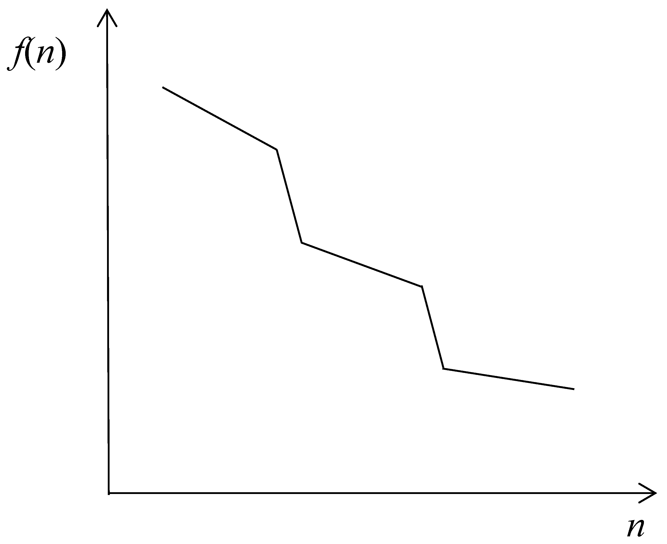
The phenomenon of service rate degradation emerges in cloud nodes and other technical services with the problem of resource contention. When a single system serves many customers, processing of their requests can slow down due to various factors (e.g., shared CPU cores and caches, memory and disk usage, etc.). In these cases, when resource utilization in a cloud node grows, we find that performance of a single task execution (request, operation, or virtual machine—VM) decreases. This phenomenon can be modeled by using degradation of service rates for the tasks executed in the node. It is obvious that such degradation depends on the number of the tasks. We may figure performance degradation of a single task while the number of tasks in the node increases, as shown in Figure 1. Here, we have intervals of small decreasing or intervals with constant performance and some points where the performance falls greatly. These points may correspond to the saturation points of some resource (see, for example, [1,2,3]).

Methods of experimental data analysis of service rate degradation in cloud nodes are described in [4], where the authors point out the negative effects of resource sharing and propose methods for simulation of the node operation. The aim of their research is to predict the performance overhead for executing services on virtualized platforms. Experiments show that the number of VMs running in the node affects the performance and its service degrades while the number of VMs grows.

Ref. [5] considers server consolidation as a factor of service rate degradation in a cloud node. The level of the degradation is defined in terms of a server consolidation overhead i.e., extra workload that the system incurs to support consolidation, regardless of the hypervisor type. Experiments depict growth of overhead while the number of VMs increases.

Since the experimental data show service rate degradation, the question arises how to estimate the extent of this degradation. In paper [6], the authors present a literature survey on performance evaluation for IAAS cloud nodes, which also encounter service rate degradation. As in the previous reference, they observe evaluation algorithms based on overhead of VMs in cloud services.

Ref. [7] focuses on measuring CPU, memory, I/O and the overall VM performance degradation caused by the performance interference of VMs sharing one physical machine. For measuring, Bayesian networks with hidden variables are used. In paper [8], the approach to performance measuring is also proposed. The authors consider the relationship among the maximal number of customers, the minimal service resources and the highest level of services. The purpose of the study is to formulate advice on the system design to meet QoS requirements. The proposed metrics can be used as a criteria for the evaluation of service rate degradation. Paper [9] is devoted to the real-time performance analysis of internet services suffering from service rate degradation. The authors propose an algorithm for evaluating the metrics on-the-fly to catch anomalies in providing service.

We have found just a few papers dedicated to the performance degradation in cloud services. The problem is well known and many authors note it. However, modeling of the systems with service rate decreasing is rare. This is because a study of such models with variable parameters is very complicated. The most popular type of models with state-dependent service rate is stepwise decreasing. For instance, we have some threshold value of the number of VMs in the physical machine. If the number of VMs is less than it, the service rate has some defined value and it equals another value if the number of VMs is greater than the threshold. Such an approach to the modeling is used, for example in papers [10,11]. In [12,13], degradation refers to aging of severs.

Another method is using modeling of service rates, arrival rates and waiting times (before service) as dependent random variables [14,15]. In [16], the queueing system with workload-dependent service and arrival rates is considered.

Unfortunately, the literature on service rate degradation modeling is mostly limited to the cases where the dependence on threshold values is considered. In our study, we propose to model a cloud node operation as a queueing system with unlimited number of servers and degradation of the service rates dependent on the number of VMs operating in the node. In addition, we take into account the following fact: in each time moment, some of VMs work actively consuming a lot of the node resources and strongly contributing to the performance degradation. On the other hand, some VMs may be in a passive (waiting) regime consuming small amount of resources. Moreover, the VMs inside the node can switch between the regimes. We model this by using the term “phase of service” (or simply “phase”) and consider a model with two phases of service (active and passive). The number of the service phases may be greater than two. However, the study of such a model requires more complex analysis. We aim to perform it in the future using the current one as the base for research.

In the paper, we take into account only the number of VMs operating inside the node for implementation of service rate degradation. Issues on taking into account detailed information on consumed resources as well as how to collect statistical data for estimation of the model parameters (including degradation functions) is outside the scope of this paper.

The salient features of the paper:

• An infinite-server queue with two phases of service and service rate degradation is proposed as a new mathematical model of a cloud node;
• An effect of service rate degradation is proposed for taking into account performance decreasing of processes in the cloud node that appears due to their contention for the node resources;
• The method of asymptotic analysis is adapted for the model and the asymptotic solution of the global balance equation is derived;
• Performed numerical experiments show good accuracy of the obtained approximation (asymptotic solution).

The rest of the paper is organized as follows. A detailed description of the mathematical model under study is presented in Section 2. In Section 3, we write a local balance equation and present its exact solution. There we establish a condition of the global and the local balance equations equivalence, which give us the applicability area of the obtained analytical (exact) solution. In Section 4, we apply the asymptotic analysis method [17,18,19] to solve the global balance equation. As the result, we derive two-dimensional Gaussian approximation of the probability distribution of the random process under study. A numerical analysis is made in Section 5. Firstly, it includes a comparison of the asymptotic and the exact distributions to establish an accuracy of the approximation and its applicability area. In addition, we present an analysis of the dependence of performance parameters on the system configuration ones.

2. Mathematical Model

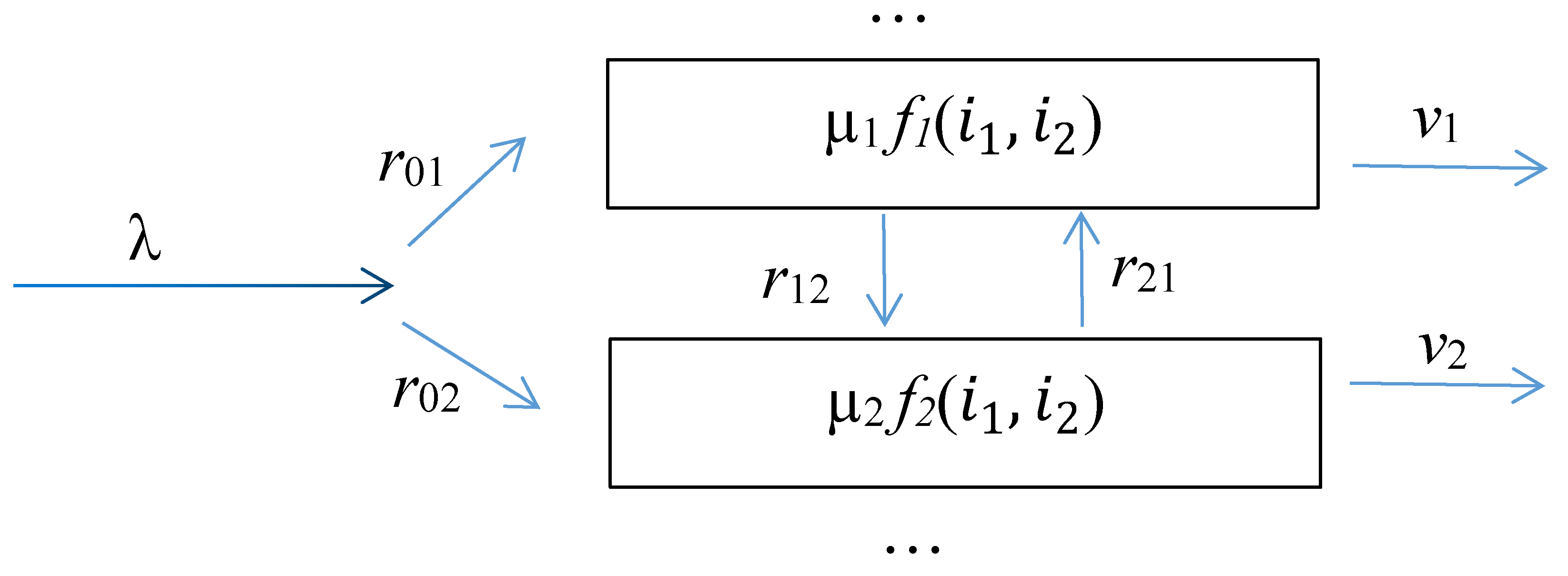
Consider a cloud node with virtual machines (VMs) operating inside it. We use an infinite-server queueing system as its model supposing that there is no queue for the VMs and all of them can work simultaneously. Actually, the term “server” in the model reflects one VM executed in the node. So, we may have potentially an unlimited number of “servers”, but performance of each of them decreases when their number grows because the node has limited capabilities (the number of CPU cores) for their parallel execution. This effect is presented in the model in the form of the service rate degradation.

Some of VMs inside the node can work in an active regime consuming a great amount of the node resources; other machines may be in a waiting (passive) regime requiring a minimal amount of resources for their work. We model this situation as two phases of the VM’s servicing. The duration of the phases reflecting the necessary time for the VM ends the current regime and switches to another one. We suppose that during a specific regime, the VM should complete all tasks assigned to it. It is obvious that when the number of VMs grows, a performance of each of them decreases due to contention for the node resources. So, we present a service rate of the VM working in phase n (where $n=1\mathrm{or}2$) in the form ${\mu }_n·f_n(i_1,i_2).$ Here, ${\mu }_n$ represents nominal service rates for the n-th phase (for the case in which only the current VM is working in the entire node). Functions $f_n(i_1,i_2)>0$ reflect an effect of service rate degradation: we suppose that they decrease while the number of VMs inside the node grows. Here, $i_1$ is the number of VMs working in the first phase, $i_2$ is the number of VMs working in the second phase. We call these functions the degradation functions. So, using this approach for the modeling, we can take into account performance degradation as well as its differentiated dependence on the number of the VMs working in different phases.

Sometimes new VMs can arrive in the node and some VMs working inside the node can leave it. We model the arrivals as a Poisson process with rate $\lambda$. At an arrival moment, the VM begins its work in the n-th phase with given probability $r_{0n}$, where $n=1,2$. Upon completion of the current phase n, the VM switches to phase k ($k=1,2$) with probability $r_{nk}$ or leaves the node with probability $v_n$. Obviously, the following equalities are true:

$$\left\{\begin{array}{c}{r}_{01}+r_{02}=1,\hfill \\ r_{12}+v_1=1,\hfill \\ r_{21}+v_2=1.\hfill \end{array}\right.$$

(1)

The structure of the model under the study is shown in Figure 2.

Let us denote the following:

• ${\mathbf{r}}_0=(r_{01},r_{02})$ is a vector of the probabilities of choosing the n-th phase at the arrival moment;
• ${\mathbf{v}}_0=(v_1,v_2)$ is a vector of the probabilities of leaving the system after the n-th phase;
• $\mathbf{R}=\left[r_{nj}\right]$ is a matrix of the probabilities of transitions between phases. Here, we assume that $r_{11}=r_{22}=0$; therefore,

  $$\mathbf{R}=\left(\begin{array}{cc}0& r_{12}\\ r_{21}& 0\end{array}\right).$$

Denote the number of VMs in the n-th phase at instant t by $i_n\left(t\right)$. The goal of the study is the obtaining of the stationary probability distribution of the number of VMs in the phases, i.e., we would like to find the stationary probability distribution of the two-dimensional stochastic process $\{i_1\left(t\right),i_2\left(t\right)\}$.

3. Balance Equations and Their Solution

Denote $P(i_1,i_2,t)=\mathrm{Pr}.\{i_1\left(t\right)=i_1,i_2\left(t\right)=i_2\}$ as the probability distribution of the number of VMs working in the first and the second phases at moment t. We derive the system of global balance equations for this distribution as follows ($i_1\ge 0,i_2\ge 0$):

$$\begin{array}{c}\frac{\partial P(i_1,i_2,t)}{\partial t}=-(\lambda +i_1{\mu }_1{f}_1(i_1,i_2)+i_2{\mu }_2{f}_2(i_1,i_2))P(i_1,i_2,t)+\\ \lambda r_{01}P(i_1-1,i_2,t)+\lambda r_{02}P(i_1,i_2-1,t)+\\ v_1(i_1+1){\mu }_1{f}_1(i_1+1,i_2)P(i_1+1,i_2,t)+\\ v_2(i_2+1){\mu }_2{f}_2(i_1,i_2+1)P(i_1,i_2+1,t)+\\ r_{12}(i_1+1){\mu }_1{f}_1(i_1+1,i_2-1)P(i_1+1,i_2-1,t)+\\ r_{21}(i_2+1){\mu }_2{f}_2(i_1-1,i_2+1)P(i_1-1,i_2+1,t).\end{array}$$

(2)

In the steady state, Equation (2) has the form

$$\begin{array}{c}-(\lambda +i_1{\mu }_1{f}_1(i_1,i_2)+i_2{\mu }_2{f}_2(i_1,i_2))P(i_1,i_2)+\lambda r_{01}P(i_1-1,i_2)+\lambda r_{02}P(i_1,i_2-1,t)+\\ v_1(i_1+1){\mu }_1{f}_1(i_1+1,i_2)P(i_1+1,i_2)+v_2(i_2+1){\mu }_2{f}_2(i_1,i_2+1)P(i_1,i_2+1)+\\ r_{12}(i_1+1){\mu }_1{f}_1(i_1+1,i_2-1)P(i_1+1,i_2-1)+\\ r_{21}(i_2+1){\mu }_2{f}_2(i_1-1,i_2+1)P(i_1-1,i_2+1).\end{array}$$

(3)

Since the direct solution of System (3) seems problematic, we propose to consider local balance equations.

In Figure 3, we show the graph of transitions between states of the two-dimensional process $\{i_1\left(t\right),i_2\left(t\right)\}$. As we can see, each cycle of the graph consists of two subcycles with three nodes. So, a solution of the local balance equations coincides with the solution of System (3) only when the following equalities are true:

$$\left\{\begin{array}{c}{r}_{01}\lambda ·r_{12}(i_1+1){\mu }_1{f}_1(i_1+1,i_2)·v_2(i_2+1){\mu }_2{f}_2(i_1,i_2+1)=\hfill \\ {\displaystyle v_1(i_1+1){\mu }_1{f}_1(i_1+1,i_2)·r_{02}\lambda ·r_{21}(i_2+1){\mu }_2{f}_2(i_1,i_2+1),}\hfill \\ {\displaystyle r_{01}\lambda ·v_2(i_2+1){\mu }_2{f}_2(i_1+1,i_2+1)·r_{12}(i_1+1){\mu }_1{f}_1(i_1+1,i_2)=}\hfill \\ {\displaystyle v_1(i_1+1){\mu }_1{f}_1(i_1+1,i_2+1)·r_{21}(i_2+1){\mu }_2{f}_2(i_1,i_2+1)·r_{02}\lambda .}\hfill \end{array}\right.$$

Thus, we obtain two conditions

$$\begin{array}{c}{r}_{01}{r}_{12}{v}_2=r_{02}{r}_{21}{v}_1,\\ {\displaystyle \frac{f_1(i_1+1,i_2)}{f_1(i_1+1,i_2+1)}=\frac{f_2(i_1,i_2+1)}{f_2(i_1+1,i_2+1)}.}\end{array}$$

(4)

From Equation (4), we can conclude that

$${\displaystyle \frac{f_1(i_1+1,i_2)}{f_1(i_1+1,i_2+1)}=\frac{f_2(i_1,i_2+1)}{f_2(i_1+1,i_2+1)}=C.}$$

(5)

Let us look at a couple of examples of the degradation functions satisfying Equation (5). This condition is true for functions $f_1(i_1,i_2)$ and $f_2(i_1,i_2)$ dependent only on the sum of the arguments, i.e.,:

$${\displaystyle f_1(i_1,i_2)=f_2(i_1,i_2)\equiv f(i_1+i_2).}$$

Another example of functions satisfying Equation (5) is the following:

$$f_1(i_1,i_2)=f_1\left(i_1\right),f_2(i_1,i_2)\equiv 1.$$

This means that we have service rate degradation in the first phase only and it does not depend on the number of VMs in the second phase.

Under conditions (4), the solution of System (3) is equal to the solution of the following local balance equations:

$$\left\{\begin{array}{c}P(i_1,i_2)r_{01}\lambda =P(i_1+1,i_2)v_1{\mu }_1(i_1+1)f_1(i_1+1,i_2),\hfill \\ P(i_1,i_2)r_{02}\lambda =P(i_1,i_2+1)v_2{\mu }_2(i_2+1)f_2(i_1,i_2+1),\hfill \\ P(i_1,i_2+1)r_{21}{\mu }_2(i_2+1)f_2(i_1,i_2+1)=P(i_1+1,i_2)r_{12}{\mu }_1(i_1+1)f_1(i_1+1,i_2).\hfill \end{array}\right.$$

(6)

Note that we have two equivalent systems of the local balance equations for two subcycles in the transition graph (Figure 3). From Equation (6), it is easy to derive that

$$\left\{\begin{array}{c}P(i_1,i_2)=P(i_1-1,i_2)\frac{{\rho }_1}{i_1{f}_1(i_1,i_2)}=\frac{{\rho }_1^{i_1}}{{\displaystyle i_1!\prod _{k=1}^{i_1}{f}_1(k,i_2)}}P(0,i_2),\\ P(i_1,i_2)=P(i_1,i_2-1)\frac{{\rho }_2}{i_2{f}_2(i_1,i_2)}=\frac{{\rho }_2^{i_2}}{{\displaystyle i_2!\prod _{k=1}^{i_2}{f}_2(i_1,k)}}P(i_1,0),\end{array}\right.$$

where

$${\rho }_1=\frac{r_{01}\lambda }{v_1{\mu }_1},{\rho }_2=\frac{r_{02}\lambda }{v_2{\mu }_2}.$$

Finally, we obtain the solution of System (6) in the following form:

$$P(i_1,i_2)=\frac{{\rho }_1^{i_1}{\rho }_2^{i_2}}{{\displaystyle i_1!i_2!\prod _{k=1}^{i_1}{f}_1(k,i_2)\prod _{m=1}^{i_2}{f}_2(i_1,m)}}P(0,0),$$

(7)

where probability $P(0,0)$ can be evaluated from the normalization condition as follows:

$$P(0,0)={\left(\sum _{i_1=0}^{\infty }\sum _{i_2=0}^{\infty }\frac{{\rho }_1^{i_1}{\rho }_2^{i_2}}{{\displaystyle i_1!i_2!\prod _{k=1}^{i_1}{f}_1(k,i_2)\prod _{m=1}^{i_2}{f}_2(i_1,m)}}\right)}^{-1}.$$

(8)

The stability condition of the system is equivalent to the conditions of the series convergence (to obtain the condition for the series convergence, the d’Alembert test is used):

$$\begin{array}{c}\frac{{\rho }_1}{(i_1+1)f_1(i_1+1,i_2)}<1,\\ \frac{{\rho }_2}{(i_2+1)f_2(i_1,i_2+1)}<1.\end{array}$$

In this way, we proved that the two-dimensional distribution of the number of VMs in the first and second phases of the queueing system with service rate degradation is not factorizable opposite to classical queueing models without any degradation.

Total Number of Virtual Machines in the Node

Let us obtain the probability distribution of the total number of VMs $i_1\left(t\right)+i_2\left(t\right)$ in the node. We derive the distribution using the following convolution:

$${\displaystyle P\left(i\right)=\sum _{l=0}^{i}P(l,i-l)=\sum _{l=0}^i\left(\frac{{\rho }_1^l{\rho }_2^{i-l}}{{\displaystyle l!(i-l)!\prod _{k=1}^l{f}_1(k,i-l)\prod _{m=1}^{i-l}{f}_2(l,m)}}P\left(0\right)\right),}$$

where $P\left(0\right)$ is calculated from the normalization condition.

4. Asymptotic Analysis

Note that Equalities (4) set a narrow applicability area of the obtained results. Therefore, we propose to obtain a solution to the problem using the asymptotic analysis method [17,18,19]. Unlike the above-mentioned papers where equations for characteristic functions are studied, in this paper, we propose an approach of a new kind, where equations for probability distributions are solved directly.

Let us find a solution to global balance equations System (3) under an asymptotic condition of growing service time [18]: ${\mu }_n\to 0,n=1,2$. We will perform the asymptotic analysis in two steps similar to the approach in [19].

4.1. First Order Asymptotics

First of all, we introduce scale parameter $T\to \infty$, which can be interpreted like a service time coefficient. Let us write the service rates in the form

$${\mu }_n=\frac{{\gamma }_n}{T},$$

(9)

where ${\gamma }_n>0$ for $n=1,2$ are some constants. Substituting Equation (9) into Equations (3), we obtain

$$\begin{array}{c}-\left(\lambda +\frac{i_1}{T}{\gamma }_1{f}_1(i_1,i_2)+\frac{i_2}{T}{\gamma }_2{f}_2(i_1,i_2)\right)P(i_1,i_2)+\lambda r_{01}P(i_1-1,i_2)+\\ \lambda r_{02}P(i_1,i_2-1,t)+v_1\frac{i_1+1}{T}{\gamma }_1{f}_1(i_1+1,i_2)P(i_1+1,i_2)+\\ v_2\frac{i_2+1}{T}{\gamma }_2{f}_2(i_1,i_2+1)P(i_1,i_2+1)+\\ r_{12}\frac{i_1+1}{T}{\gamma }_1{f}_1(i_1+1,i_2-1)P(i_1+1,i_2-1)+\\ r_{21}\frac{i_2+1}{T}{\gamma }_2{f}_2(i_1-1,i_2+1)P(i_1-1,i_2+1).\end{array}$$

(10)

Denote

$$\begin{array}{c}\epsilon =\frac{1}{T},\frac{i_n}{T}=i_n\epsilon =x_n,\\ P(i_1,i_2)=\tilde{P}(x_1,x_2,\epsilon ),\\ P(i_1-1,i_2)=\tilde{P}(x_1-\epsilon ,x_2,\epsilon ),\\ f_n(i_1,i_2)={\tilde{f}}_n(x_1,x_2)\end{array}$$

(11)

where $\epsilon$ is an infinitesimal value (suppose $\epsilon \to 0$).

Substituting Notations (11) into Equation (10), we obtain the following equation

$$\begin{array}{c}-(\lambda +x_1{\gamma }_1{\tilde{f}}_1(x_1,x_2)+x_2{\gamma }_2{\tilde{f}}_2(x_1,x_2))\tilde{P}(x_1,x_2,\epsilon )+\lambda r_{01}\tilde{P}(x_1-\epsilon ,x_2,\epsilon )+\\ \lambda r_{02}\tilde{P}(x_1,x_2-\epsilon ,\epsilon )+v_1(x_1+\epsilon ){\gamma }_1{\tilde{f}}_1(x_1+\epsilon ,x_2)\tilde{P}(x_1+\epsilon ,x_2,\epsilon )+\\ {\displaystyle v_2(x_2+\epsilon ){\gamma }_2{\tilde{f}}_2(x_1,x_2+\epsilon )\tilde{P}(x_1,x_2+\epsilon ,\epsilon )+}\\ r_{12}(x_1+\epsilon ){\gamma }_1{\tilde{f}}_1(x_1+\epsilon ,x_2-\epsilon )\tilde{P}(x_1+\epsilon ,x_2-\epsilon ,\epsilon )+\\ r_{21}(x_2+\epsilon ){\gamma }_2{\tilde{f}}_2(x_1-\epsilon ,x_2+\epsilon )\tilde{P}(x_1-\epsilon ,x_2+\epsilon ,\epsilon ).\end{array}$$

(12)

Let us use the following series representations of the functions:

$$\begin{array}{c}\tilde{P}(x_1-\epsilon ,x_2,\epsilon )=\tilde{P}(x_1,x_2,\epsilon )-\epsilon \frac{\partial \tilde{P}(x_1,x_2,\epsilon )}{\partial x_1}+O\left({\epsilon }^2\right),\\ (x_1+\epsilon ){\tilde{f}}_1(x_1+\epsilon ,x_2)\tilde{P}(x_1+\epsilon ,x_2,\epsilon )=\\ x_1{\tilde{f}}_1(x_1,x_2)\tilde{P}(x_1,x_2,\epsilon )+\epsilon \frac{\partial \left(x_1{\tilde{f}}_1(x_1,x_2)\tilde{P}(x_1,x_2,\epsilon )\right)}{\partial x_1}+O\left({\epsilon }^2\right),\\ (x_1+\epsilon ){\tilde{f}}_1(x_1+\epsilon ,x_2-\epsilon )\tilde{P}(x_1+\epsilon ,x_2-\epsilon ,\epsilon )=x_1{\tilde{f}}_1(x_1,x_2)\tilde{P}(x_1,x_2,\epsilon )+\\ \epsilon \frac{\partial \left(x_1{\tilde{f}}_1(x_1,x_2)\tilde{P}(x_1,x_2,\epsilon )\right)}{\partial x_1}-\epsilon x_1\frac{\partial \left({\tilde{f}}_1(x_1,x_2)\tilde{P}(x_1,x_2,\epsilon )\right)}{\partial x_2}+O\left({\epsilon }^2\right),\end{array}$$

(13)

where $O\left({\epsilon }^2\right)$ is infinitesimal value of order ${\epsilon }^2$.

Writing a similar expression for other terms, substituting Expressions (13) into Equation (12) and taking into account Equalities (1), we obtain the following equation:

$$\begin{array}{c}-\epsilon \lambda r_{01}\frac{\partial \tilde{P}(x_1,x_2,\epsilon ))}{\partial x_1}-\epsilon \lambda r_{02}\frac{\partial \tilde{P}(x_1,x_2,\epsilon ))}{\partial x_2}+\\ \epsilon v_1{\gamma }_1\frac{\partial \left(x_1{\tilde{f}}_1(x_1,x_2)\tilde{P}(x_1,x_2,\epsilon )\right)}{\partial x_1}+\epsilon v_2{\gamma }_2\frac{\partial \left(x_2{\tilde{f}}_2(x_1,x_2)\tilde{P}(x_1,x_2,\epsilon )\right)}{\partial x_2}+\\ \epsilon r_{12}{\gamma }_1\frac{\partial \left(x_1{\tilde{f}}_1(x_1,x_2)\tilde{P}(x_1,x_2,\epsilon )\right)}{\partial x_1}-\epsilon r_{12}{\gamma }_1{x}_1\frac{\partial \left({\tilde{f}}_1(x_1,x_2)\tilde{P}(x_1,x_2,\epsilon )\right)}{\partial x_2}+\\ {\displaystyle \epsilon r_{21}{\gamma }_2{x}_2\frac{\partial \left({\tilde{f}}_2(x_1,x_2)\tilde{P}(x_1,x_2,\epsilon )\right)}{\partial x_1}-\epsilon r_{21}{\gamma }_2\frac{\partial \left(x_2{\tilde{f}}_2(x_1,x_2)\tilde{P}(x_1,x_2,\epsilon )\right)}{\partial x_2}=O\left({\epsilon }^2\right).}\end{array}$$

(14)

After that, we divide the equation by $\epsilon$ and take the limit transition by $\epsilon \to 0$. Taking into account Equalities (1), we have the following degenerate Fokker–Planck equation for stationary distribution $\tilde{P}(x_1,x_2)$:

$$\begin{array}{c}\frac{\partial }{\partial x_1}\left((-\lambda r_{01}+{\gamma }_1{x}_1{\tilde{f}}_1(x_1,x_2)-r_{21}{\gamma }_2{x}_2{\tilde{f}}_2(x_1,x_2))\tilde{P}(x_1,x_2)\right)+\\ \frac{\partial }{\partial x_2}\left((-\lambda r_{02}+{\gamma }_2{x}_2{\tilde{f}}_2(x_1,x_2)-r_{12}{\gamma }_1{x}_1{\tilde{f}}_1(x_1,x_2))\tilde{P}(x_1,x_2)\right)=0.\end{array}$$

(15)

The diffusion coefficient for the degenerate Fokker–Planck equation is equal to zero, which means that asymptotic processes $x_1\left(t\right)$ and $x_2\left(t\right)$ are deterministic. To obtain the stationary distribution, we write the following system

$$\begin{array}{c}{\displaystyle -\lambda r_{01}+{\gamma }_1{x}_1{\tilde{f}}_1(x_1,x_2)-r_{21}{\gamma }_2{x}_2{\tilde{f}}_2(x_1,x_2)=0,}\hfill \\ {\displaystyle -\lambda r_{02}+{\gamma }_2{x}_2{\tilde{f}}_2(x_1,x_2)-r_{12}{\gamma }_1{x}_1{\tilde{f}}_1(x_1,x_2)=0,}\hfill \end{array}$$

(16)

Let functions ${\tilde{f}}_1(x_1,x_2)$ and ${\tilde{f}}_2(x_1,x_2)$ satisfy a condition when only a single solution of System (16) exists (searching this condition requires special studies and lays out of the scope of the paper). Denote the solution of Equations (16) as

$$x_1={\kappa }_1,x_2={\kappa }_2.$$

Values ${\kappa }_1$ and ${\kappa }_2$ define the asymptotic normalized means of random processes $i_1\left(t\right)$ and $i_2\left(t\right)$.

4.2. Second Order Asymptotics

Denote

$$\begin{array}{c}{\epsilon }^2=\frac{1}{T},\frac{i_n}{T}=i_n{\epsilon }^2=x_n+\epsilon y_n,\\ \frac{i_n+1}{T}=(i_n+1){\epsilon }^2=x_n+\epsilon (y_n+\epsilon ),P(i_1,i_2)=\tilde{\tilde{P}}(y_1,y_2,\epsilon ),\\ P(i_1-1,i_2)=\tilde{\tilde{P}}(y_1-\epsilon ,y_2,\epsilon ),\\ f_n(i_1,i_2)={\tilde{\tilde{f}}}_n(x_1+\epsilon y_1,x_2+\epsilon y_2)\end{array}$$

(17)

where $\epsilon$ is an infinitesimal value (in limit $\epsilon \to 0$).

Substituting Equation (17) into Equation (10), we obtain

$$\begin{array}{c}-(\lambda +(x_1+\epsilon y_1){\gamma }_1{\tilde{\tilde{f}}}_1(x_1+\epsilon y_1,x_2+\epsilon y_2)+(x_2+\epsilon y_2){\gamma }_2{\tilde{\tilde{f}}}_2(x_1+\epsilon y_1,x_2+\epsilon y_2))\tilde{\tilde{P}}(y_1,y_2,\epsilon )+\\ \lambda r_{01}\tilde{\tilde{P}}(y_1-\epsilon ,y_2,\epsilon )+\lambda r_{02}\tilde{\tilde{P}}(y_1,y_2-\epsilon ,\epsilon )+\\ v_1(x_1+\epsilon (y_1+\epsilon )){\gamma }_1{\tilde{\tilde{f}}}_1(x_1+\epsilon (y_1+\epsilon ),x_2+\epsilon y_2)\tilde{\tilde{P}}(y_1+\epsilon ,y_2,\epsilon )+\\ v_2(x_2+\epsilon (y_2+\epsilon )){\gamma }_2{\tilde{\tilde{f}}}_2(x_1+\epsilon y_1,x_2+\epsilon (y_2+\epsilon )\tilde{\tilde{P}}(y_1,y_2+\epsilon ,\epsilon )+\\ r_{12}(x_1+\epsilon (y_1+\epsilon )){\gamma }_1{\tilde{\tilde{f}}}_1(x_1+\epsilon (y_1+\epsilon ),x_2+\epsilon (y_2-\epsilon ))\tilde{\tilde{P}}(y_1+\epsilon ,y_2-\epsilon ,\epsilon )+\\ r_{21}(x_2+\epsilon (y_2+\epsilon )){\gamma }_2{\tilde{\tilde{f}}}_2(x_1+\epsilon (y_1-\epsilon ),x_2+\epsilon (y_2+\epsilon ))\tilde{\tilde{P}}(y_1-\epsilon ,y_2+\epsilon ,\epsilon )=0.\end{array}$$

(18)

We use the following series expansions for the functions:

$$\begin{array}{c}\tilde{\tilde{P}}(y_1-\epsilon ,y_2,\epsilon )=\tilde{\tilde{P}}(y_1,y_2,\epsilon )-\epsilon \frac{\partial \tilde{\tilde{P}}(y_1,y_2,\epsilon )}{\partial y_1}+\frac{{\epsilon }^2}{2}\frac{{\partial }^2\tilde{\tilde{P}}(y_1,y_2,\epsilon )}{\partial y_1^2}+O\left({\epsilon }^3\right),\\ (x_1+\epsilon (y_1+\epsilon )){\tilde{\tilde{f}}}_1(x_1+\epsilon (y_1+\epsilon ),x_2+\epsilon y_2)\tilde{\tilde{P}}(y_1+\epsilon ,y_2,\epsilon )=\\ (x_1+\epsilon y_1){\tilde{\tilde{f}}}_1(x_1+\epsilon ,x_2+\epsilon y_2)\tilde{\tilde{P}}(y_1,y_2,\epsilon )+\epsilon (x_1+\epsilon y_1)\frac{\partial (y_1{\tilde{\tilde{f}}}_1(x_1+\epsilon ,x_2+\epsilon y_2)\tilde{\tilde{P}}(y_1,y_2,\epsilon )}{\partial y_1}+\\ \frac{{\epsilon }^2}{2}{x}_1\frac{{\partial }^2\left(y_1{\tilde{\tilde{f}}}_1(x_1+\epsilon y_1,x_2+\epsilon y_2)\tilde{\tilde{P}}(y_1,y_2,\epsilon )\right)}{\partial y_1^2}+O\left({\epsilon }^3\right),\\ (x_1+\epsilon (y_1+\epsilon )){\tilde{\tilde{f}}}_1(x_1+\epsilon (y_1+\epsilon ),x_2+\epsilon (y_2-\epsilon ))\tilde{\tilde{P}}(y_1+\epsilon ,y_2-\epsilon ,\epsilon )=\\ (x_1+\epsilon y_1){\tilde{\tilde{f}}}_1(x_1+\epsilon y_1,x_2+\epsilon y_2)\tilde{\tilde{P}}(y_1,y_2,\epsilon )+\epsilon \frac{\partial \left((x_1+\epsilon y_1){\tilde{\tilde{f}}}_1(x_1+\epsilon y_1,x_2+\epsilon y_2)\tilde{\tilde{P}}(y_1,y_2,\epsilon )\right)}{\partial y_1}-\\ \epsilon \frac{\partial ((x_1+\epsilon y_1){\tilde{\tilde{f}}}_1(x_1+\epsilon y_1,x_2+\epsilon y_2)\tilde{\tilde{P}}(y_1,y_2,\epsilon )}{\partial y_2}+\\ \frac{{\epsilon }^2}{2}\frac{{\partial }^2\left(x_1{\tilde{\tilde{f}}}_1(x_1+\epsilon y_1,x_2+\epsilon y_2)\tilde{\tilde{P}}(y_1,y_2,\epsilon )\right)}{\partial y_1^2}+\frac{{\epsilon }^2}{2}\frac{{\partial }^2\left(x_1{\tilde{\tilde{f}}}_1(x_1+\epsilon y_1,x_2+\epsilon y_2)\tilde{\tilde{P}}(y_1,y_2,\epsilon )\right)}{\partial y_2^2}-\\ {\epsilon }^2\frac{{\partial }^2\left(x_1{\tilde{\tilde{f}}}_1(x_1+\epsilon y_1,x_2+\epsilon y_2)\tilde{\tilde{P}}(y_1,y_2,\epsilon )\right)}{\partial y_1\partial y_2}+O\left({\epsilon }^3\right),\end{array}$$

(19)

Substituting Equation (19) (and similar ones for the other terms) into Equation (18) and making some transformations, after dividing by $\epsilon$, we obtain

$$\begin{array}{c}\frac{\partial }{\partial y_1}\left(\left(-\lambda r_{01}+{\gamma }_1(x_1+\epsilon y_1){\tilde{\tilde{f}}}_1(x_1+\epsilon y_1,x_2+\epsilon y_2)-\right.\right.\\ \left.\left.r_{21}{\gamma }_2(x_2+\epsilon y_2){\tilde{\tilde{f}}}_2(x_1+\epsilon y_1,x_2+\epsilon y_2)\right)\tilde{\tilde{P}}(y_1,y_2,\epsilon )\right)+\\ \frac{\partial }{\partial y_2}\left(\left(-\lambda r_{02}+{\gamma }_2(x_2+\epsilon y_2){\tilde{\tilde{f}}}_1(x_1+\epsilon y_1,x_2+\epsilon y_2)-\right.\right.\\ \left.\left.r_{12}{\gamma }_1(x_1+\epsilon y_{)}{\tilde{\tilde{f}}}_2(x_1+\epsilon y_1,x_2+\epsilon y_2)\right)\tilde{\tilde{P}}(y_1,y_2,\epsilon )\right)+\\ \frac{\epsilon }{2}\frac{{\partial }^2}{\partial y_1^2}\left(\left(\lambda r_{01}+v_1{\gamma }_1{x}_1{\tilde{\tilde{f}}}_1(x_1+\epsilon y_1,x_2+\epsilon y_2)+r_{12}{\gamma }_1{x}_1{\tilde{\tilde{f}}}_1(x_1+\epsilon y_1,x_2+\epsilon y_2)+\right.\right.\\ \left.\left.r_{21}{\gamma }_2{x}_2{\tilde{\tilde{f}}}_2(x_1+\epsilon y_1,x_2+\epsilon y_2)\right)\tilde{\tilde{P}}(y_1,y_2,\epsilon )\right)+\\ \frac{\epsilon }{2}\frac{{\partial }^2}{\partial y_2^2}\left(\left(\lambda r_{02}+v_2{\gamma }_2{x}_2{\tilde{\tilde{f}}}_2(x_1+\epsilon y_1,x_2+\epsilon y_2)+r_{12}{\gamma }_1{x}_1{\tilde{\tilde{f}}}_1(x_1+\epsilon y_1,x_2+\epsilon y_2)+\right.\right.\\ \left.\left.r_{21}{\gamma }_2{x}_2{\tilde{\tilde{f}}}_2(x_1+\epsilon y_1,x_2+\epsilon y_2)\right)\tilde{\tilde{P}}(y_1,y_2,\epsilon )\right)-\epsilon \frac{{\partial }^2}{\partial y_1\partial y_2}\left(\left(r_{12}{\gamma }_1{x}_1{\tilde{\tilde{f}}}_1(x_1+\epsilon y_1,x_2+\epsilon y_2)+\right.\right.\\ \left.\left.r_{21}{\gamma }_2{x}_2{\tilde{\tilde{f}}}_2(x_1+\epsilon y_1,x_2+\epsilon y_2)\right)\tilde{\tilde{P}}(y_1,y_2,\epsilon )\right)=O\left({\epsilon }^2\right).\end{array}$$

(20)

Moreover, we use the expansions for functions ${\tilde{\tilde{f}}}_n(x_1+\epsilon y_1,x_2+\epsilon y_2)$ by $x_1$ and $x_2$ as in Equation (13).

Finally, we have the following equation for $\epsilon \to 0$:

$$\begin{array}{c}\frac{\partial }{\partial y_1}\left(\tilde{\tilde{P}}(y_1,y_2)\left({\gamma }_1{y}_1\frac{\partial \left(x_1{\tilde{\tilde{f}}}_1(x_1,x_2)\right)}{\partial x_1}+{\gamma }_1{y}_1\frac{\partial \left(x_1{\tilde{\tilde{f}}}_1(x_1,x_2)\right)}{\partial x_2}-\right.\right.\\ \left.\left.r_{21}{\gamma }_2{y}_1\frac{\partial \left(x_2{\tilde{\tilde{f}}}_2(x_1,x_2)\right)}{\partial x_1}-r_{21}{\gamma }_2{y}_2\frac{\partial \left(x_2{\tilde{\tilde{f}}}_2(x_1,x_2)\right)}{\partial x_2}\right)\right)+\\ \frac{\partial }{\partial y_2}\left(\tilde{\tilde{P}}(y_1,y_2)\left({\gamma }_2{y}_1\frac{\partial \left(x_2{\tilde{\tilde{f}}}_2(x_1,x_2)\right)}{\partial x_1}+{\gamma }_2{y}_2\frac{\partial \left(x_2{\tilde{\tilde{f}}}_2(x_1,x_2)\right)}{\partial x_2}-\right.\right.\\ {\displaystyle \left.\left.r_{12}{\gamma }_1{y}_1\frac{\partial \left(x_1{\tilde{\tilde{f}}}_1(x_1,x_2)\right)}{\partial x_1}-r_{12}{\gamma }_1{y}_2\frac{\partial \left(x_1{\tilde{\tilde{f}}}_1(x_1,x_2)\right)}{\partial x_2}\right)\right)+}\\ \frac{1}{2}\frac{{\partial }^2}{\partial y_1^2}\left(\tilde{\tilde{P}}(y_1,y_2)\left(\lambda r_{01}+v_1{\gamma }_1{x}_1{\tilde{\tilde{f}}}_1(x_1,x_2)+r_{12}{\gamma }_1{x}_1{\tilde{\tilde{f}}}_1(x_1,x_2)+r_{21}{\gamma }_2{x}_2{\tilde{\tilde{f}}}_2(x_1,x_2)\right)\right)+\\ \frac{1}{2}\frac{{\partial }^2}{\partial y_2^2}\left(\tilde{\tilde{P}}(y_1,y_2)\left(\lambda r_{02}+v_2{\gamma }_2{x}_2{\tilde{\tilde{f}}}_2(x_1,x_2)+r_{12}{\gamma }_1{x}_1{\tilde{\tilde{f}}}_1(x_1,x_2)+r_{21}{\gamma }_2{x}_2{\tilde{\tilde{f}}}_2(x_1,x_2)\right)\right)-\\ \frac{{\partial }^2}{\partial y_1\partial y_2}\left(\tilde{\tilde{P}}(y_1,y_2)\left(r_{12}{\gamma }_1{x}_1{\tilde{\tilde{f}}}_1(x_1,x_2)+r_{21}{\gamma }_2{x}_2{\tilde{\tilde{f}}}_2(x_1+,x_2)\right)\right)=0.\end{array}$$

(21)

Let us introduce the following notations in Equation (21):

$$\begin{array}{c}{a}_{11}=\frac{\partial }{\partial x_1}\left({\gamma }_1{x}_1{\tilde{\tilde{f}}}_1(x_1,x_2)-r_{21}{\gamma }_2{x}_2\tilde{\tilde{f}}(x_1,x_2)\right),\\ a_{12}=\frac{\partial }{\partial x_2}\left({\gamma }_1{x}_1{\tilde{\tilde{f}}}_1(x_1,x_2)-r_{21}{\gamma }_2{x}_2\tilde{\tilde{f}}(x_1,x_2)\right),\\ a_{21}=\frac{\partial }{\partial x_1}\left({\gamma }_2{x}_2{\tilde{\tilde{f}}}_2(x_1,x_2)-r_{12}{\gamma }_1{x}_1\tilde{\tilde{f}}(x_1,x_2)\right),\\ a_{22}=\frac{\partial }{\partial x_2}\left({\gamma }_2{x}_2{\tilde{\tilde{f}}}_2(x_1,x_2)-r_{12}{\gamma }_1{x}_1\tilde{\tilde{f}}(x_1,x_2)\right),\\ b_1={\gamma }_1{x}_1{\tilde{\tilde{f}}}_2(x_1,x_2),\\ b_2={\gamma }_2{x}_2{\tilde{\tilde{f}}}_2(x_1,x_2),\\ b_{12}=r_{12}{\gamma }_1{x}_1{\tilde{\tilde{f}}}_1(x_1,x_2)+r_{21}{\gamma }_2{x}_2{\tilde{\tilde{f}}}_2(x_1,x_2).\end{array}$$

(22)

Thus, we obtain the following Fokker–Planck equation for two-dimensional probability density $\tilde{\tilde{P}}(y_1,y_2)$:

$$\begin{array}{c}\frac{\partial }{\partial y_1}\left(\tilde{\tilde{P}}(y_1,y_2)(y_1{a}_{11}+y_2{a}_{12})\right)+\frac{\partial }{\partial y_2}\left(\tilde{\tilde{P}}(y_1,y_2)(y_1{a}_{21}+y_2{a}_{22})\right)+\\ \frac{{\partial }^2}{\partial y_1^2}\left(\tilde{\tilde{P}}(y_1,y_2)b_1\right)+\frac{{\partial }^2}{\partial y_2^2}\left(\tilde{\tilde{P}}(y_1,y_2)b_2\right)-\frac{{\partial }^2}{\partial y_1\partial y_2}\left(\tilde{\tilde{P}}(y_1,y_2)b_{12}\right)=0,\end{array}$$

(23)

where coefficients $a_{11},a_{12},a_{21},a_{22},b_1,b_2,b_{12}$ are evaluated for $x_1={\kappa }_1$, $x_2={\kappa }_2$, which are the solution of Equation (16).

Making the inverse Fourier transform yields the asymptotic characteristic function

$${\displaystyle H(u_1,u_2)={\int }_{-\infty }^{\infty }{\int }_{-\infty }^{\infty }{e}^{j{u}_1{y}_1}{e}^{j{u}_2{y}_2}\tilde{\tilde{P}}(y_1,y_2)d{y}_{1}d{y}_2.}$$

Taking into account properties of the inverse Fourier transform, we rewrite Equation (23) as follows:

$$\begin{array}{c}{\displaystyle \frac{\partial H(u_1,u_2)}{\partial u_1}(u_1{a}_{11}+u_2{a}_{12})+\frac{\partial H(u_1,u_2)}{\partial u_2}(u_1{a}_{21}+u_2{a}_{22})+}\\ {\displaystyle H(u_1,u_2)\left(u_1^2{b}_1+u_2^2{b}_2-u_1{u}_2{b}_{12}\right)=0.}\end{array}$$

(24)

Obviously, the solution of Equation (24) has the following form:

$${\displaystyle H(u_1,u_2)=exp\left\{-\frac{1}{2}{u}_1^2{K}_{11}-u_1{u}_2{K}_{12}-\frac{1}{2}{u}_2^2{K}_{22}\right\},}$$

where

$$\begin{array}{c}{K}_{11}=\frac{b_1-K_{12}{a}_{12}}{a_{11}},\\ K_{22}=\frac{b_2-K_{12}{a}_{21}}{a_{22}},\\ K_{12}=\frac{a_{11}{a}_{22}{b}_{12}+a_{21}{a}_{22}{b}_1+a_{12}{a}_{11}{b}_2}{(a_{11}+a_{22})(a_{21}{a}_{12}-a_{11}{a}_{22})}.\end{array}$$

(25)

Thus, we can conclude that the asymptotic distribution of the number of VMs in the phases is two-dimensional Gaussian with density function

$$\begin{array}{c}{\displaystyle p(x_1,x_2)=\frac{1}{2\pi \sqrt{K_{11}{K}_{22}(1-{\eta }^2)}}\times }\\ {\displaystyle exp\left\{-\frac{1}{2(1-{\eta }^2)}\left(\frac{{(x_1-{\kappa }_1)}^2}{K_{11}}-\eta \frac{2(x_1-{\kappa }_1)(x_2-{\kappa }_2)}{\sqrt{K_{11}{K}_{22}}}+\frac{{(x_2-{\kappa }_2)}^2}{K_{22}}\right)\right\}}\end{array}$$

(26)

where a correlation coefficient given by

$${\displaystyle \eta =\sqrt{\frac{K_{12}}{K_{11}{K}_{22}}}}$$

and other parameters defined in Equations (16), (22) and (25).

4.3. Asymptotic Result on the Total Number of Virtual Machines in the Node

Let us write the asymptotic probability distribution of the total number of VMs $i_1\left(t\right)+i_2\left(t\right)$ in the considered queueing system:

$${\displaystyle p\left(x\right)=\frac{1}{\sigma \sqrt{2\pi }}exp\left\{-\frac{1}{2}\frac{{(x-m)}^2}{\sigma }\right\},}$$

(27)

where

$$m={\kappa }_1+{\kappa }_2,\sigma =K_{11}+K_{22}+2\sqrt{K_{12}}.$$

Remark. Gaussian distributions (26) and (27) are continuous probability distributions defined for negative arguments too. For obtaining the discrete probability distributions of the considered processes, the following formula may be used:

$$p_{\mathrm{discrete}}\left(i\right)=\frac{p\left(i\right)}{{\sum }_{i=0}^{\infty }p\left(i\right)},$$

(28)

only for $i\ge 0$.

Moreover, we should take into account that obtained results Equations (26), (27) and (28) are approximate. Thus, we need to establish their accuracy and applicability area. This is done in the next section.

5. Numerical Examples

For the demonstration of the results as well as for estimating an accuracy of the obtained approximation, we consider an example of the queueing system with the Poisson arrival process, an unlimited number of servers and two phases of service. Service rate degradation is only in the first phase (i.e., $f_2(x_1,x_2)\equiv 1$) and depends on the number of VMs working in the first phase only (i.e., $f_1(x_1,x_2)\equiv f_1\left(x_1\right)$). Parameters for the example are the following:

$$\lambda =0.005,\mathbf{v}={(0.1,0.1)}^T,{\mathbf{r}}_0=(0.5,0.5),\mathbf{R}=\left(\begin{array}{cc}0& 0.9\\ 0.9& 0\end{array}\right),$$

$${\mu }_1={\gamma }_1/T,{\mu }_2={\gamma }_2/T,{\gamma }_1=1,{\gamma }_2=2,$$

where T is variable (it is necessary for analysis of the applicability area of the asymptotic results).

We consider two examples of service rate degradation function in the first phase:

$$\left(\mathrm{a}\right)f_1\left(x_1\right)=\frac{1}{\sqrt{1+x_1}},\left(\mathrm{b}\right)f_1\left(x_1\right)=\frac{1}{\pi }arctan\left(2(x_1-2)\right).$$

(29)

The forms of the degradation functions are presented in Figure 4.

The results obtained in Section 3 will serve us as standard on sets of the parameters satisfied conditions (4). Comparing the exact solution (7) with the asymptotic approximation (26) on such sets of parameters, we can determine the asymptotic method application area. Condition (4) is true for parameters defined above.

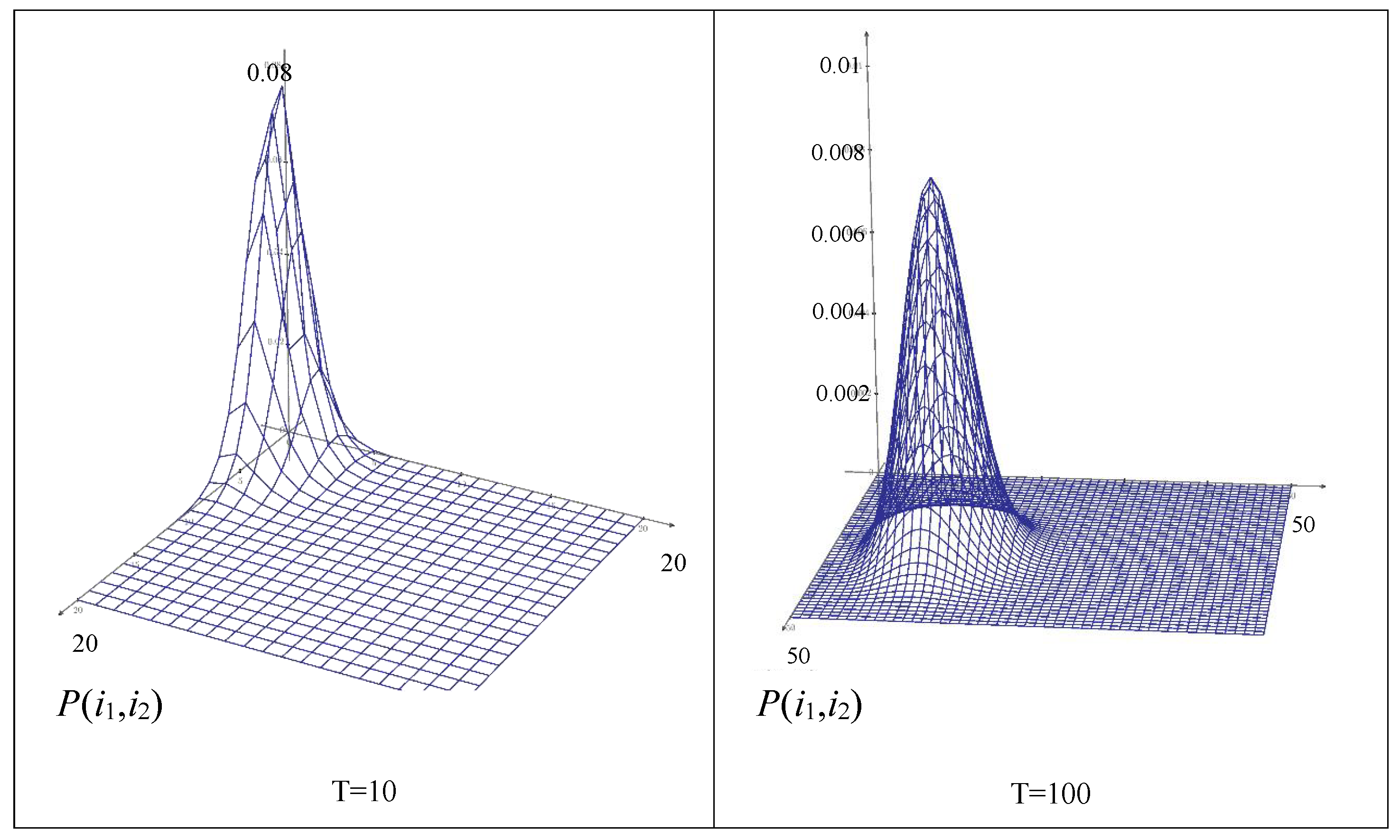
First of all, we present the exact two-dimensional probability distribution of the number of VMs in each phase in cases where $T=10$ and $T=100$. Figure 5 shows the results for the example with degradation function (29a).

In this case, exact one-dimensional distributions of the number of VMs in each phase and the total number of VMs in the system have the forms shown in Figure 6. Means and variance of the distributions are presented in

Table 1. Means and variance of the probability distributions.

	E$\left\{\mathit{P}1\right(\mathit{i}\left)\right\}$	E$\left\{\mathit{P}2\right(\mathit{i}\left)\right\}$	E$\left\{\mathit{P}\mathit{s}\mathit{u}\mathit{m}\right(\mathit{i}\left)\right\}$	var$\left\{\mathit{P}\mathit{s}\mathit{u}\mathit{m}\right(\mathit{i}\left)\right\}$
$T=10$	2.937	1.250	4.187	4.555
$T=100$	27.484	12.500	39.984	40.408

.

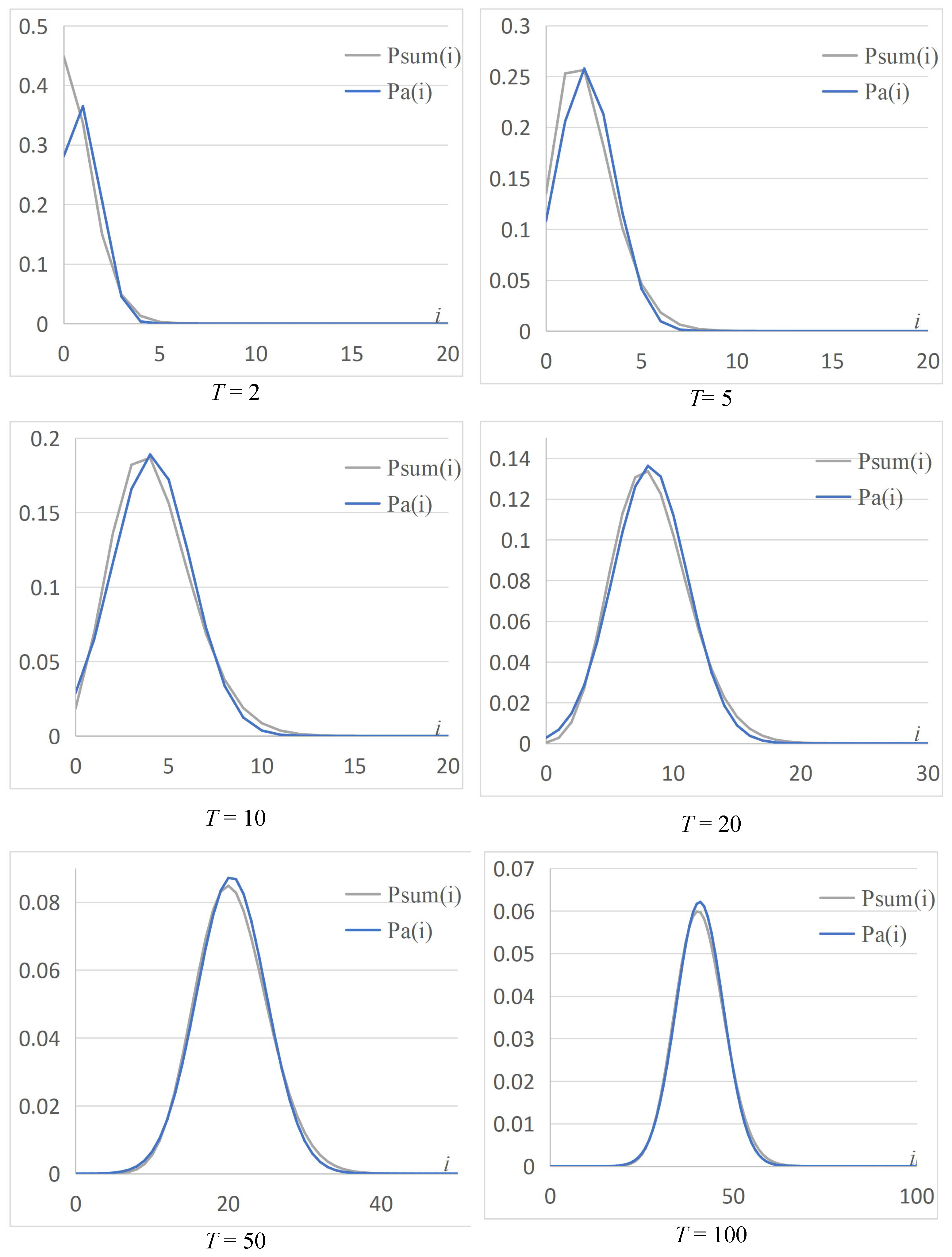
In Figure 7, we show examples of the comparison of the asymptotic and the exact distributions for different values of T. For making conclusions about the precision of the asymptotic result and its applicability area, we compare the exact and the asymptotic distributions of the total number of VMs for different values of parameter T for both types of degradation function (29). We use Kolmogorov distance as a measure of the difference between the distributions:

$$\delta =\underset{i\ge 0}{max}\left|\sum _{l=0}^i\left[P\left(k\right)-Pa\left(k\right)\right]\right|,$$

(30)

where $P\left(k\right)$ is the exact probability distribution; $Pa\left(k\right)$ is the corresponding asymptotic one. Values of the Kolmogorov distances are presented in

Table 2. Values of the Kolmogorov distances.

T	1	2	5	10	20	50	100
${\delta }_{\left(a\right)}$	0.256	0.168	0.074	0.030	0.017	0.016	0.014
${\delta }_{\left(b\right)}$	0.184	0.148	0.102	0.049	0.013	0.013	0.010

. Supposing that an error $\delta \le 0.05$ is acceptable, we may conclude that the asymptotic formulas can be applied for values $T\ge 10$. The advantage of the asymptotic method is the absence of conditions on the system parameters, so it can be applied for a wide area of values of the system parameters.

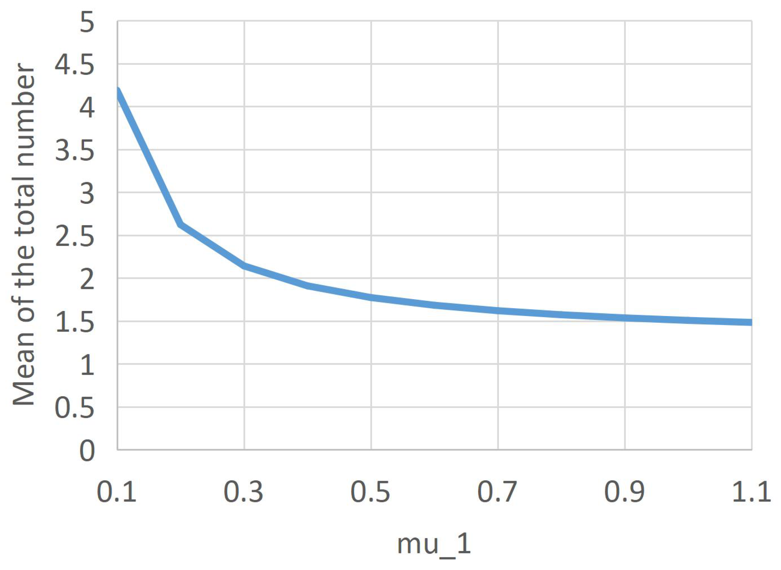
In addition, we show the dependency of the mean of the total number of VMs in the system on the following model parameters:

• arrival rate $\lambda$;
• service rate ${\mu }_1$;
• parameter a of the degradation function ${\displaystyle f_1\left(x_1\right)=\frac{1}{\pi }arctan\left(2(x_1-a)\right)}$.

The results are presented in Figure 8, Figure 9 and Figure 10.

6. Discussion

In the paper, we have considered the queueing model with an unlimited number of servers and service rate degradation depending on the number of customers in the system. Such a model may be useful for modeling of systems where a growing number of customers leads to lower performance for each customer. For example, in a cloud node, when the number of executed virtual machines (VMs) grows, their individual performance decreases due to contention for shared resources (CPU cores, caches, memory, etc.). In addition, in the proposed model, customers may be served in two phases with different service parameters (including degradation functions) switching between the phases. This feature help us to model different behavior of VMs in different states as well as different requirements for resources in these states. For example, there is an active phase when a VM performs some executions (processing requests) and a passive phase when the VM is in a sleep mode or waiting for requests.

Studying the model, we derived the system of global balance Equation (3) for the steady-state regime. The system cannot be solved directly. Therefore, we tried to solve it using an equivalence Condition (4) between global and local balance solutions. Solutions (7) and (8) were derived but the equivalence condition seems very strong and does not allow one to apply the solution in a wide class of the systems.

Due to this fact, we applied the asymptotic analysis method to obtain an approximate solution of System (3). The condition of growing service time is used for the asymptotic analysis. The approach similar to [17,18,19] is used, but unlike the mentioned papers, here we performed a direct study of the probability distribution function instead of an analysis of characteristic functions. As a result, we derived two-dimensional Gaussian approximation (26) of the distribution of the number of VMs in the phases of service.

Theoretically, the obtained approximation should become more precise when the service time grows (the asymptotic condition). So, we need to establish whether it works in such a way and estimate the approximation precision for different parameters. These results are presented in Section 5. There we performed a numerical analysis of the obtained results by comparing approximation (26) with exact solution (7) and (8) for the case when Condition (4) is satisfied. Using the Kolmogorov distance as an error estimation, we found that the error decreases when the average service time grows. The visual presentation of the distributions in Figure 7 confirms this conclusion.

Future studies may be devoted to considering similar models with the number of service phases greater than 2. Moreover, the problem of deriving requirements for degradation functions which ensure the existence of only a single solution of system (16) is important. This problem may become dramatic when the number of phases and the number of degradation functions and their arguments increase greatly.

References

1. Patros, P.; Kent, K.B.; Dawson, M. SLO request modeling, reordering and scaling. In Proceedings of the 27th Annual International Conference on Computer Science and Software Engineering, Markham, ON, Canada, 6–8 November 2017; pp. 180–191. [Google Scholar]
2. Zhu, J.; Patros, P.; Kent, K.B.; Dawson, M. Node.js Scalability Investigation in the Cloud. In Proceedings of the 28th Annual International Conference on Computer Science and Software Engineering, Markham, ON, Canada, 29–31 October 2018; pp. 201–212. [Google Scholar]
3. Grohmann, J.; Nicholson, P.K.; Iglesias, J.O.; Kounev, S.; Lugones, D. Monitorless: Predicting Performance Degradation in Cloud Applications with Machine Learning. In Proceedings of the 20th International Middleware Conference, Davis, CA, USA, 9–13 December 2019; pp. 149–162. [Google Scholar]
4. Huber, N.; von Quast, M.; Brosig, F.; Hauck, M.; Kounev, S. A Method for Experimental Analysis and Modeling of Virtualization Performance Overhead. In Cloud Computing and Services Science. CLOSER 2011. Service Science: Research and Innovations in the Service Economy; Springer: Berlin/Heidelberg, Germany, 2012; pp. 353–370. [Google Scholar]
5. Bermejo, B.; Juiz, C. A general method for evaluating the overhead when consolidating servers: Performance degradation in virtual machines and containers. J. Supercomput. 2022, 78, 11345–11372. [Google Scholar] [CrossRef]
6. Xu, F.; Liu, F.; Jin, H.; Vasilakos, A.V. Managing performance overhead of virtual machines in cloud computing: A survey, state of the art and future directions. Proc. IEEE 2013, 102, 11–31. [Google Scholar] [CrossRef]
7. Hao, J.; Zhang, B.; Yue, K.; Wu, H.; Zhang, J. Measuring performance degradation of virtual machines based on the Bayesian network with hidden variables. Int. J. Commun. Syst. 2018, 31, e3732. [Google Scholar] [CrossRef]
8. Xiong, K.; Perros, H. Service performance and analysis in cloud computing. In Proceedings of the 2009 Congress on Services—I, Los Angeles, CA, USA, 6–10 July 2009; pp. 693–700. [Google Scholar]
9. Ibidunmoye, O.; Metsch, T.; Elmroth, E. Real-time detection of performance anomalies for cloud services. In Proceedings of the IEEE/ACM 24th International Symposium on Quality of Service (IWQoS), Beijing, China, 20–21 June 2016; pp. 1–2. [Google Scholar]
10. Liu, X.; Li, S.; Tong, W. A queuing model considering resources sharing for cloud service performance. J. Supercomput. 2015, 71, 4042–4055. [Google Scholar] [CrossRef]
11. Goswami, V.; Patra, S.S.; Mund, G.B. Performance analysis of cloud with queue-dependent virtual machines. In Proceedings of the 2012 1st International Conference on Recent Advances in Information Technology (RAIT), Dhanbad, India, 15–17 March 2012; pp. 357–362. [Google Scholar]
12. Choudhary, A.; Chakravarthy, S.R.; Sharma, D.C. Analysis of MAP/PH/1 Queueing System with Degrading Service Rate and Phase Type Vacation. Mathematics 2021, 9, 2387. [Google Scholar] [CrossRef]
13. Ejaz, I.; Alvarado, M.; Gautam, N.; Gebraeel, N.; Lawley, M. Condition-Based Maintenance for Queues With Degrading Servers. IEEE Trans. Autom. Sci. Eng. 2019, 16, 1750–1762. [Google Scholar] [CrossRef]
14. Morozov, E. Stability Analysis of a General State-Dependent Multiserver Queue. J. Math. Sci. 2014, 200, 462–472. [Google Scholar] [CrossRef]
15. Boxma, O.J.; Perry, D. A queueing model with dependence between service and interarrival times. Eur. J. Oper. Res. 128 2008, 3, 611–624. [Google Scholar]
16. Bekker, R. Finite-buffer queues with workload-dependent service and arrival rates. Queueing Syst. 2005, 50, 231–253. [Google Scholar] [CrossRef] [Green Version]
17. Nazarov, A.; Paul, S.; Lizyura, O. Asymptotic analysis of Markovian retrial queue with unreliable server and multiple types of outgoing calls. Glob. Stoch. Anal. 2021, 8, 143–149. [Google Scholar]
18. Moiseeva, S.P.; Bushkova, T.V.; Pankratova, E.V.; Farkhadov, M.P.; Imomov, A.A. Asymptotic analysis of the resource heterogeneous QS (MMPP+2M)(2,ν)/GI(2)/ under the condition of an equivalently growing service time. Avtomat. I Telemekh. 2022, 8, 81–99. [Google Scholar]
19. Danilyuk, E.; Moiseeva, S.; Nazarov, A. Asymptotic Diffusion Analysis of an Retrial Queueing System M/M/1 with Impatient Calls. Commun. Comput. Inf. Sci. 2022, 1552, 233–246. [Google Scholar]
Figure 1. Degradation of a single VM performance f ( n ) vs. growing of the number of VMs inside the node n.
Axioms 12 00104 g001
Figure 2. A queueing system with two phases of service and service rate degradation.
Axioms 12 00104 g002
Figure 3. Graph of transitions for process { i 1 ( t ) , i 2 ( t ) } .
Axioms 12 00104 g003
Figure 4. Service rate degradation functions.
Axioms 12 00104 g004
Figure 5. Two-dimensional probability distributions of the number of VMs in the phases of service.
Axioms 12 00104 g005
Figure 6. Probability distributions of the number of VMs in the 1st phase P 1 ( i ) , in the 2nd phase P 2 ( i ) and the total number of VMs in the system P s u m ( i ) .
Axioms 12 00104 g006
Figure 7. The comparison of asymptotic distribution P a ( i ) and exact distribution P s u m ( i ) .
Axioms 12 00104 g007
Figure 8. Mean of the total number of VMs vs. the arrival rate λ .
Axioms 12 00104 g008
Figure 9. Mean of the total number of VMs vs. service rate parameter μ 1 in the first phase.
Axioms 12 00104 g009
Figure 10. Mean of the total number of VMs vs. parameter a of the degradation function.
Axioms 12 00104 g010