
Statistical Inference of the Beta Binomial Exponential 2 Distribution with Application to Environmental Data

Abstract
1. Introduction
- (i)
- Provide a generalization of the distribution by including two additional shape parameters that allow for larger adaptability in the form of the beta binomial exponential 2 () distribution and, as a result, in modeling observed positive data.
- (ii)
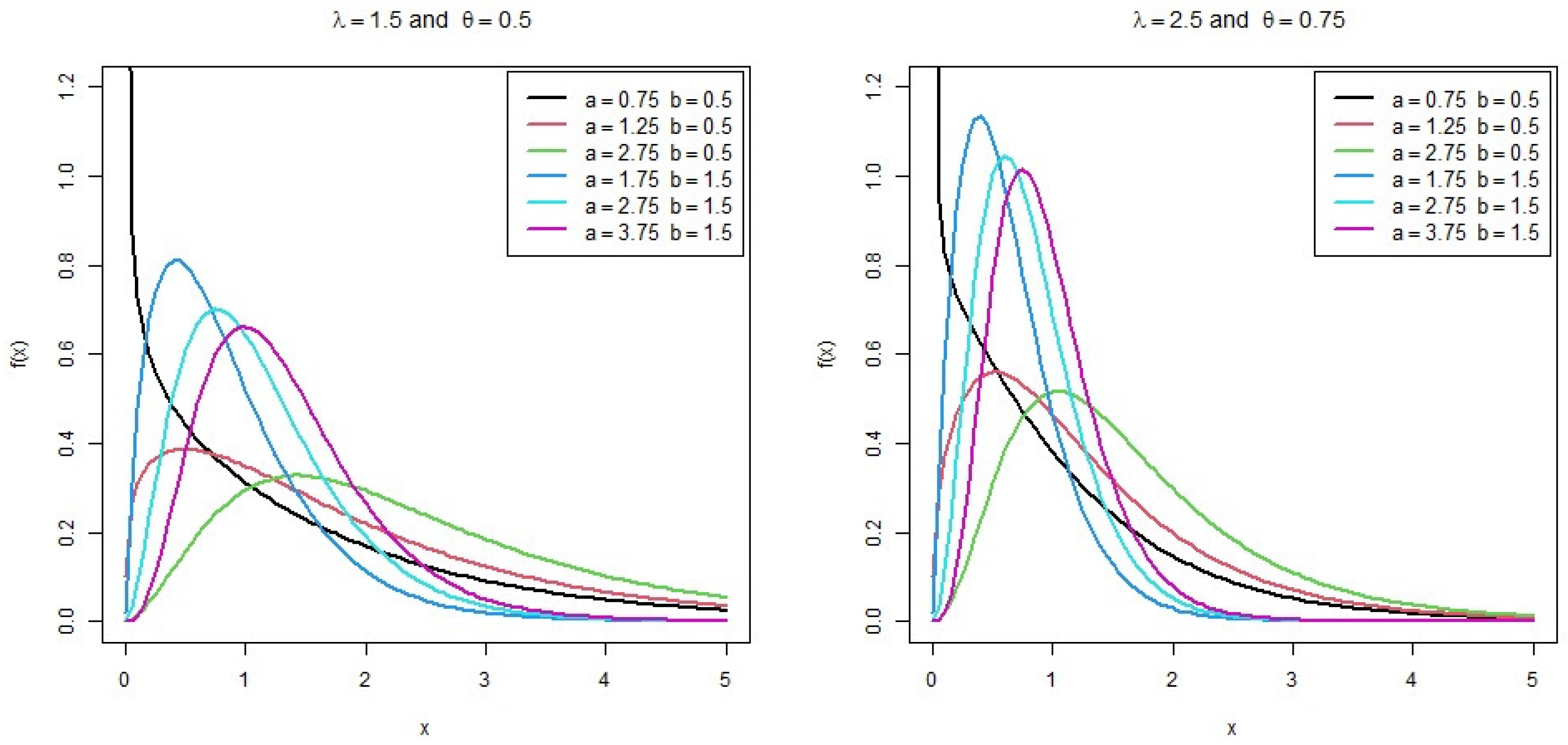
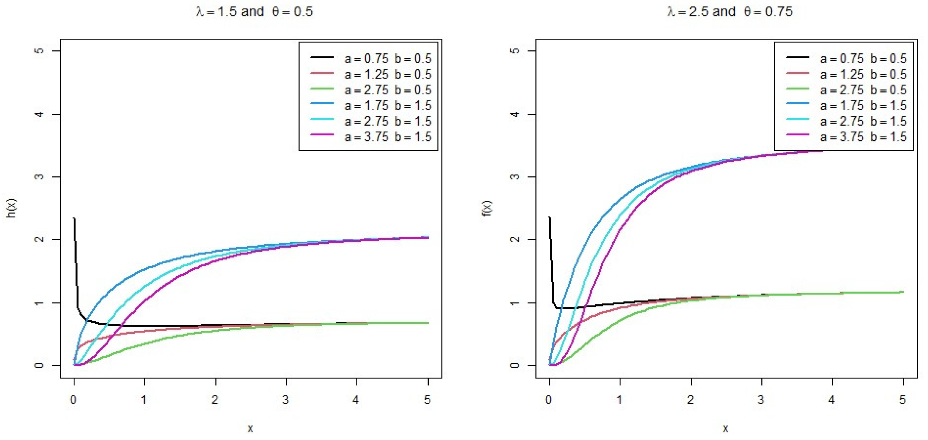
- The pdf of the distribution can take different shapes, such as decreasing, unimodal and right skewness, and the shapes of the hazard rate function (hrf) can be decreasing, increasing and constant.
- (iii)
- Some statistical and mathematical features of the distribution are computed and investigated.
- (iv)
- Develop an acceptance sampling plan (ASP), derive its operating characteristic function and give the corresponding decision rule by using the distribution.
- (v)
- Study two classical approaches of estimation; maximum likelihood () and maximum product of spacing (). Further, the Bayesian approach of estimation is utilized to estimate the model parameters.
- (vi)
- The significance of the model is demonstrated through a study of real-world data applications, which demonstrates the flexibility and potential of the model in comparison to other well-known competitive models.
2. Beta Binomial Exponential 2 Distribution
A Useful Representation
3. Statistical Features of the Distribution
3.1. Quantile Function
3.2. Moments
3.3. Moment-Generating Function
4. Acceptance Sampling Plans
- Take n units at random from the suggested lot as a sample.
- Run the following test for units of time:If c or fewer units (acceptance number) fail during the test, accept the entire lot; otherwise, the lot is rejected.
- ,
- ,
- (note that when )
- The parameters of the BBE2 distribution are assumed to be:
- Case 1:
- Case 2:
- Parameter of the BBE2 distribution is assumed to be and .
- For the parameters of ASP: When and c are increasing, the required sample size n is increasing, but is decreasing. While k is increasing, the required n is decreasing, but is increasing.
- For the parameters of the distribution: With increases in any parameters of and b where the other parameters are fixed, the required n is increasing, but is decreasing.
5. Non-Bayesian Estimation Methods
5.1. Maximum Likelihood Estimation
5.2. Maximum Product of Spacing Estimation
6. Bayesian Estimation
6.1. Markov Chain Monte Carlo
- Starting with an initial guess: just one value that could be gathered from the distribution.
- Creating a series of new samples based on this first guess. Each new sample is created in two steps:
- Proposal: A new sample proposal is produced by adding a small random disturbance to the most recent sample.
- Acceptance: The suggestion is either accepted as the new sample or rejected (in which case the old sample is retained).
6.2. Metropolis–Hasting Algorithm
- Step 1.
- Set initial value of as .
- Step 2.
- For repeat the next stages:
- 2.1:
- Set .
- 2.2:
- Generate a new candidate parameter value from .
- 2.3:
- Set .
- 2.4:
- Calculate , where is the posterior density in (23).
- 2.5:
- Generate a sample u from the uniform distribution.
- 2.6:
- Accept or reject the new candidate
6.3. Highest Posterior Density Intervals
7. Simulation Study and Data Analysis
Simulation Study
- Sample size generated from the distribution is supposed to be .
- For the parameters of the beta distribution, we assumed that: and .
- For parameter of the exponential distribution, we assumed that: .
- For parameter of the binomial distribution, we assumed that: .
- In general, the increasing n, MSEs and AILs are decreasing for all methods of Non-BEs and BEs. Further, two Non-BEs methods (MLE and MPSP) are competing well for estimating the parameters of the distribution. For BE methods, the loss function GE estimates are better than BEs under other loss functions (LINEX and SE).
- For fixed and as the value of b increases, the MSEs of and b estimates are increasing, but the MSEs of and a are decreasing.
- For fixed and as the value of a increases, the MSEs of and estimates are decreasing, but the MSEs of a and b are increasing.
- For fixed and as the value of increases, the MSEs of estimates is decreasing, but the MSEs of a and b are increasing.
- For fixed and as the value of increases, the MSEs of all parameters are increasing.
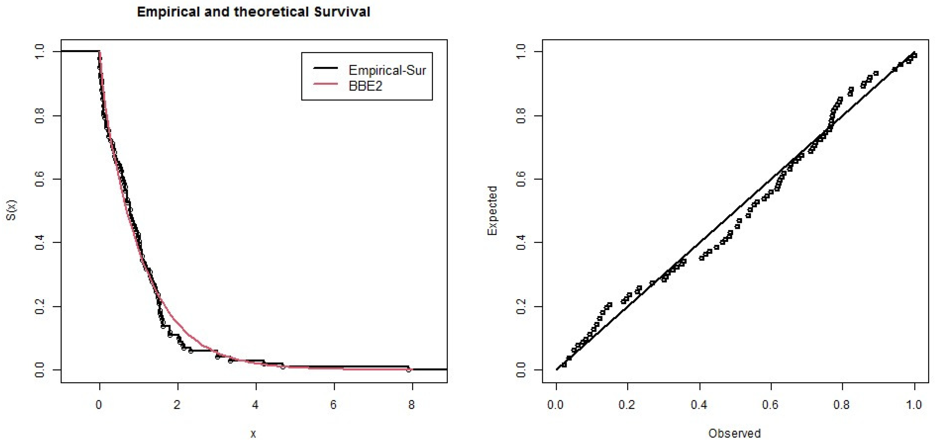
8. Applications: Kevlar Data
9. Conclusions
Author Contributions
Funding
Data Availability Statement
Acknowledgments
Conflicts of Interest
References
- Shaked, M.; Shanthikumar, J.G. Stochastic Orders; Springer: New York, NY, USA, 2007. [Google Scholar]
- Barlow, R.E.; Proschan, F. Statistical Theory of Reliability and Life Testing; Holt, Rinehart, and Winston: New York, NY, USA, 1975. [Google Scholar]
- Bakouch, H.S.; Jazi, M.A.; Nadarajah, S.; Dolati, A.; Roozegar, R. A lifetime model with increasing failure rate. Appl. Math. Modell. 2014, 38, 5392–5406. [Google Scholar] [CrossRef]
- Singh, K.P.; Lee, C.M.; George, E.O. On generalized log-logistic model for censored survival data. Biom. J. 1998, 30, 843–850. [Google Scholar] [CrossRef]
- Eugene, C.; Lee, F. Beta-normal distribution and its applications. Commun. Stat. Theory Methods 2002, 31, 497–512. [Google Scholar] [CrossRef]
- Nadarajah, S.; Kotz, S. The beta Gumbel distribution. Math. Probl. Eng. 2004, 10, 323–332. [Google Scholar] [CrossRef]
- Nadarajah, S.; Gupta, A. The beta Frechet distribution. Far East J. Theor. Stat. 2004, 14, 15–24. [Google Scholar]
- Lee, C.; Famoye, F.; Olumolade, O. Beta-Weibull Distribution: Some Properties and Applications to Censored Data. J. Modern Appl. Statist. Methods 2007, 6, 173–186. [Google Scholar] [CrossRef]
- Bidram, H.; Behboodian, J.; Towhidi, M. The beta Weibull-geometric distribution. J. Statist. Comput. Simul. 2013, 83, 52–67. [Google Scholar] [CrossRef]
- Barreto-Souza, W.; Santos, A.; Cordeiro, G.M. The beta generalized exponential distribution. J. Statist. Comput. Simul. 2010, 80, 159–172. [Google Scholar] [CrossRef]
- Silva, G.O.; Ortega, E.M.M.; Cordeiro, G.M. The beta modified Weibull distribution. Lifetime Data Anal. 2010, 16, 409–430. [Google Scholar] [CrossRef]
- Khan, M.S. The beta inverse Weibull distribution. Int. Trans. Math. Sci. Comput. 2010, 3, 113–119. [Google Scholar]
- Mahmoudi, E. The Beta Generalized Pareto distribution with application to lifetime data. Math. Compu. Simul. 2011, 81, 2414–2430. [Google Scholar] [CrossRef]
- Cordeiro, G.M.; Gomes, A.E.; da-Silva, C.Q.; Ortega, E.M.M. The beta exponentiated Weibull distribution. J. Statist. Comput. Simul. 2013, 83, 114–138. [Google Scholar] [CrossRef]
- Haq, M.; Elgarhy, M. The odd Fréchet- G family of probability distributions. J. Stat. Appl. Probab. 2018, 7, 189–203. [Google Scholar] [CrossRef]
- Cordeiro, G.; Ortega, E.; da Cunha, D.C. The exponentiated generalized class of distributions. J. Data Sci. 2013, 11, 1–27. [Google Scholar] [CrossRef]
- Zubair, A.; Elgarhy, M.; Hamedani, G.; Butt, N. Odd generalized N-H generated family of distributions with application to exponential model. Pak. J. Stat. Oper. Res. 2020, 16, 53–71. [Google Scholar]
- Alzaatreh, A.; Lee, C.; Famoye, F. A new method for generating families of continuous distributions. Metron 2013, 71, 63–79. [Google Scholar] [CrossRef]
- Aldahlan, M.A.; Jamal, F.; Chesneau, C.; Elbatal, I.; Elgarhy, M. Exponentiated power generalized Weibull power series family of distributions: Properties, estimation and applications. PLoS ONE 2020, 15, e0230004. [Google Scholar] [CrossRef]
- Bourguignon, M.; Silva, R.B.; Cordeiro, G.M. The Weibull-G family of probability distributions. J. Data Sci. 2014, 12, 1253–1268. [Google Scholar] [CrossRef]
- Hassan, A.S.; Elgarhy, M.; Shakil, M. Type II half Logistic family of distributions with applications. Pak. J. Stat. Oper. Res. 2017, 13, 245–264. [Google Scholar]
- Alotaibi, N.; Elbatal, I.; Almetwally, E.M.; Alyami, S.A.; Al-Moisheer, A.S.; Elgarhy, M. Truncated Cauchy Power Weibull-G Class of Distributions: Bayesian and Non-Bayesian Inference Modelling for COVID-19 and Carbon Fiber Data. Mathematics 2022, 10, 1565. [Google Scholar] [CrossRef]
- Elbatal, I.; Alotaibi, N.; Almetwally, E.M.; Alyami, S.A.; Elgarhy, M. On Odd Perks-G Class of Distributions: Properties, Regression Model, Discretization, Bayesian and Non-Bayesian Estimation, and Applications. Symmetry 2022, 14, 883. [Google Scholar] [CrossRef]
- Algarni, A.; MAlmarashi, A.; Elbatal, I.; SHassan, A.; Almetwally, E.M.; MDaghistani, A.; Elgarhy, M. Type I half logistic Burr XG family: Properties, Bayesian, and non-Bayesian estimation under censored samples and applications to COVID-19 data. Math. Probl. Eng. 2021. [Google Scholar] [CrossRef]
- Al-Babtain, A.A.; Elbatal, I.; Chesneau, C.; Elgarhy, M. Sine Topp-Leone-G family of distributions: Theory and applications. Open Phys. 2020, 18, 74–593. [Google Scholar] [CrossRef]
- Bantan, R.A.; Jamal, F.; Chesneau, C.; Elgarhy, M. A New Power Topp–Leone Generated Family of Distributions with Applications. Entropy 2019, 21, 1177. [Google Scholar] [CrossRef]
- Bantan, R.A.; Jamal, F.; Chesneau, C.; Elgarhy, M. Truncated inverted Kumaraswamy generated family of distributions with applications. Entropy 2019, 21, 1089. [Google Scholar] [CrossRef]
- Mahdavi, A.; Kundu, D. A new method for generating distributions with an application to exponential distribution. Commun. Stat. Theory Methods 2017, 46, 6543–6557. [Google Scholar] [CrossRef]
- Bantan, R.A.; Chesneau, C.; Jamal, F.; Elgarhy, M. On the Analysis of New COVID-19 Cases in Pakistan Using an Exponentiated Version of the M Family of Distributions. Mathematics 2020, 8, 953. [Google Scholar] [CrossRef]
- Badr, M.M.; Elbatal, I.; Jamal, F.; Chesneau, C.; Elgarhy, M. The transmuted odd Fréchet-G family of distributions: Theory and applications. Mathematics 2020, 8, 958. [Google Scholar] [CrossRef]
- Gradshteyn, I.S.; Ryzhik, I.M. Table of Integrals, Series, and Products; Academic Press: San Diego, CA, USA, 2007. [Google Scholar]
- Asgharzadeh, A.; Bakouch, H.S.; Habibi, M. A generalized binomial exponential 2 distribution. Modeling and applications to hydrologic events. J. Appl. Stat. 2017, 44, 2368–2387. [Google Scholar] [CrossRef]
- Nadarajah, S.; Kotz, S. The beta exponential distribution. Reliab. Eng. Syst. Saf. 2006, 91, 689–697. [Google Scholar] [CrossRef]
- Kong, L.; Lee, L.; Sepanski, J. On the Properties of Beta-Gamma Distribution. J. Modern Appl. Statist. Methods 2007, 1, 187–211. [Google Scholar] [CrossRef]
- Abushal, T.A.; Hassan, A.S.; El-Saeed, A.R.; Nassr, S.G. Power Inverted Topp-Leone in Acceptance Sampling Plans. Comput. Mater. Contin. 2021, 67, 991–1011. [Google Scholar] [CrossRef]
- Alyami, S.A.; Elgarhy, M.; Elbatal, I.; Almetwally, E.M.; Alotaibi, N.; El-Saeed, A.R. Fréchet Binomial Distribution: Statistical Properties, Acceptance Sampling Plan, Statistical Inference and Applications to Lifetime Data. Axioms 2022, 11, 389. [Google Scholar] [CrossRef]
- Nassr, S.G.; Hassan, A.S.; Alsultan, R.; El-Saeed, A.R. Acceptance sampling plans for the three-parameter inverted Topp–Leone model. Math. Biosci. Eng. 2022, 19, 13628–13659. [Google Scholar] [CrossRef]
- Singh, S.; Tripathi, Y.M. Acceptance sampling plans for inverse Weibull distribution based on truncated life test. Life Cycle Reliab. Saf. Eng. 2017, 6, 169–178. [Google Scholar]
- Varian, H.R. A Bayesian approach to real estate assessment. In Variants in Economic Theory: Selected Works of H. R.Varian; Varian, H.R., Ed.; Edward Elgar Publishing: Northampton, MA, USA, 2000; Chapter 9; pp. 144–155. [Google Scholar]
- Doostparast, M.; Akbari, M.G.; Balakrishna, N. Bayesian analysis for the two-parameter Pareto distribution based on record values and times. J. Stat. Comput. Simul. 2011, 81, 1393–1403. [Google Scholar] [CrossRef]
- Calabria, R.; Pulcini, G. Point estimation under asymmetric loss functions for left-truncated exponential samples. Commun. Stat. Theory Methods 1996, 25, 585–600. [Google Scholar] [CrossRef]
- van Ravenzwaaij, D.; Cassey, P.; Brown, S.D. A simple introduction to Markov Chain Monte-Carlo sampling. Psychon. Bull. Rev. 2018, 25, 143–154. [Google Scholar] [CrossRef]
- Andrews, D.F.; Herzberg, A.M. Data: A Collection of Problems from Many Fields for the Student and Research Worker; Springer Series in Statistics; Springer: New York, NY, USA, 1985. [Google Scholar]
- Cooray, K.; Ananda, M.M.A. A generalization of the half-normal distribution with applications to life time data. Comm. Statist. Theory Methods 2008, 37, 1323–1337. [Google Scholar] [CrossRef]
- Mdlongwa, P.; Oluyede, B.O.; Amey, A.K.A.; Fagbamigbe, A.F.; Makubate, B. Kumaraswamy log-logistic Weibull distribution: Model, theory and application to lifetime and survival data. Heliyon 2019, 5, e01144. [Google Scholar] [CrossRef]


| a | b | Distribution | Authors | ||
|---|---|---|---|---|---|
| − | − | − | 1 | generalized | [32] |
| − | − | 1 | 1 | [3] | |
| − | 0 | − | − | B exponential | [33] |
| − | 2 | − | − | B gamma | [34] |
| − | 0 | 1 | 1 | exponential | |
| − | 2 | 1 | 1 | gamma |
| Moments () | ||||
|---|---|---|---|---|
| (0.5, 0.7, 0.30, 3.0) | (2.5, 2.7, 1.0, 3.0) | (1.5, 2.7, 0.70, 3.0) | (1.5, 2.7, 1.00, 3.0) | |
| 0.362942 | 0.571999 | 2.92529 | 0.435659 | |
| 0.358767 | 0.388811 | 9.50626 | 0.245108 | |
| 0.554513 | 0.30641 | 76.2397 | 0.168439 | |
| 1.14747 | 0.274943 | 550.099 | 0.136526 | |
| 2.95521 | 0.277046 | 4696.42 | 0.127411 | |
| 9.07734 | 0.310069 | 46206.3 | 0.1345 | |
| Variance | 0.22704 | 0.061628 | 0.948911 | 0.0553086 |
| Skewness | 2.39872 | 0.882932 | 46.3885 | 1.03515 |
| Kurtosis | 164.972 | 13.4627 | 50623.0 | 3.9319 |
| c | 1 | |||||||||||
|---|---|---|---|---|---|---|---|---|---|---|---|---|
| and | ||||||||||||
| 0.25 | 0 | 2 | 0.8315 | 2 | 0.7634 | 1 | 1.0000 | 1 | 1.0000 | 1 | 1.0000 | |
| 1 | 6 | 0.8002 | 5 | 0.7607 | 3 | 0.8912 | 3 | 0.7944 | 3 | 0.7500 | ||
| 5 | 26 | 0.7640 | 19 | 0.7623 | 14 | 0.7673 | 10 | 0.8288 | 9 | 0.8555 | ||
| 10 | 52 | 0.7683 | 38 | 0.7560 | 27 | 0.7912 | 20 | 0.8076 | 19 | 0.7597 | ||
| 20 | 107 | 0.7579 | 77 | 0.7556 | 56 | 0.7533 | 41 | 0.7738 | 37 | 0.7975 | ||
| 0.75 | 0 | 8 | 0.2748 | 6 | 0.2593 | 4 | 0.3010 | 3 | 0.2987 | 3 | 0.2500 | |
| 1 | 16 | 0.2536 | 11 | 0.2756 | 8 | 0.2699 | 6 | 0.2510 | 5 | 0.3125 | ||
| 5 | 43 | 0.2669 | 31 | 0.2531 | 22 | 0.2595 | 16 | 0.2520 | 14 | 0.2905 | ||
| 10 | 76 | 0.2612 | 54 | 0.2604 | 38 | 0.2804 | 28 | 0.2516 | 25 | 0.2706 | ||
| 20 | 140 | 0.2585 | 99 | 0.2657 | 71 | 0.2581 | 51 | 0.2696 | 46 | 0.2757 | ||
| 0.95 | 0 | 17 | 0.0522 | 12 | 0.0513 | 8 | 0.0607 | 5 | 0.0892 | 5 | 0.0625 | |
| 1 | 27 | 0.0517 | 19 | 0.0510 | 13 | 0.0567 | 9 | 0.0608 | 8 | 0.0625 | ||
| 5 | 60 | 0.0529 | 42 | 0.0544 | 29 | 0.0616 | 21 | 0.0520 | 18 | 0.0717 | ||
| 10 | 98 | 0.0502 | 69 | 0.0501 | 48 | 0.0566 | 34 | 0.0576 | 30 | 0.0680 | ||
| 20 | 168 | 0.0526 | 119 | 0.0502 | 84 | 0.0515 | 59 | 0.0619 | 53 | 0.0632 | ||
| and | ||||||||||||
| 0.25 | 0 | 10 | 0.7641 | 4 | 0.7855 | 2 | 0.8107 | 1 | 1.0000 | 1 | 1.0000 | |
| 1 | 33 | 0.7572 | 13 | 0.7635 | 6 | 0.7591 | 3 | 0.8343 | 3 | 0.7500 | ||
| 5 | 144 | 0.7531 | 55 | 0.7626 | 23 | 0.7747 | 11 | 0.8217 | 9 | 0.8555 | ||
| 10 | 294 | 0.7512 | 113 | 0.7515 | 47 | 0.7569 | 23 | 0.7506 | 19 | 0.7597 | ||
| 20 | 604 | 0.7521 | 231 | 0.7545 | 96 | 0.7502 | 45 | 0.7874 | 37 | 0.7975 | ||
| 0.75 | 0 | 47 | 0.2528 | 18 | 0.2545 | 7 | 0.2840 | 3 | 0.3516 | 3 | 0.2500 | |
| 1 | 91 | 0.2531 | 34 | 0.2644 | 14 | 0.2638 | 6 | 0.3249 | 5 | 0.3125 | ||
| 5 | 251 | 0.2526 | 95 | 0.2568 | 38 | 0.2734 | 17 | 0.3081 | 14 | 0.2905 | ||
| 10 | 441 | 0.2513 | 167 | 0.2556 | 68 | 0.2540 | 31 | 0.2650 | 25 | 0.2706 | ||
| 20 | 809 | 0.2517 | 307 | 0.2543 | 125 | 0.2522 | 57 | 0.2681 | 46 | 0.2757 | ||
| 0.95 | 0 | 101 | 0.0503 | 38 | 0.0509 | 15 | 0.0530 | 6 | 0.0733 | 5 | 0.0625 | |
| 1 | 160 | 0.0502 | 60 | 0.0515 | 24 | 0.0511 | 10 | 0.0650 | 8 | 0.0625 | ||
| 5 | 355 | 0.0501 | 134 | 0.0503 | 53 | 0.0543 | 23 | 0.0635 | 18 | 0.0717 | ||
| 10 | 573 | 0.0503 | 216 | 0.0515 | 86 | 0.0551 | 38 | 0.0610 | 30 | 0.0680 | ||
| 20 | 983 | 0.0501 | 372 | 0.0502 | 149 | 0.0532 | 67 | 0.0536 | 53 | 0.0632 | ||
| c | 1 | |||||||||||
|---|---|---|---|---|---|---|---|---|---|---|---|---|
| and | ||||||||||||
| 0.25 | 0 | 2 | 0.8413 | 2 | 0.7752 | 1 | 1.0000 | 1 | 1.0000 | 1 | 1.0000 | |
| 1 | 7 | 0.7559 | 5 | 0.7801 | 4 | 0.7606 | 3 | 0.7986 | 3 | 0.7500 | ||
| 5 | 28 | 0.7503 | 20 | 0.7589 | 14 | 0.7948 | 10 | 0.8360 | 9 | 0.8555 | ||
| 10 | 56 | 0.7510 | 40 | 0.7532 | 28 | 0.7873 | 21 | 0.7541 | 19 | 0.7597 | ||
| 20 | 114 | 0.7508 | 81 | 0.7542 | 58 | 0.7518 | 41 | 0.7913 | 37 | 0.7975 | ||
| 0.75 | 0 | 9 | 0.2509 | 6 | 0.2800 | 4 | 0.3169 | 3 | 0.3038 | 3 | 0.2500 | |
| 1 | 17 | 0.2530 | 12 | 0.2546 | 8 | 0.2921 | 6 | 0.2580 | 5 | 0.3125 | ||
| 5 | 46 | 0.2602 | 32 | 0.2724 | 23 | 0.2513 | 16 | 0.2638 | 14 | 0.2905 | ||
| 10 | 81 | 0.2571 | 57 | 0.2576 | 40 | 0.2597 | 28 | 0.2674 | 25 | 0.2706 | ||
| 20 | 149 | 0.2552 | 105 | 0.2536 | 73 | 0.2741 | 52 | 0.2516 | 46 | 0.2757 | ||
| 0.95 | 0 | 18 | 0.0530 | 12 | 0.0608 | 8 | 0.0684 | 6 | 0.0509 | 5 | 0.0625 | |
| 1 | 28 | 0.0573 | 20 | 0.0516 | 13 | 0.0665 | 9 | 0.0640 | 8 | 0.0625 | ||
| 5 | 64 | 0.0520 | 44 | 0.0569 | 31 | 0.0508 | 21 | 0.0565 | 18 | 0.0717 | ||
| 10 | 104 | 0.0511 | 72 | 0.0550 | 50 | 0.0551 | 34 | 0.0640 | 30 | 0.0680 | ||
| 20 | 179 | 0.0513 | 125 | 0.0525 | 87 | 0.0530 | 60 | 0.0576 | 53 | 0.0632 | ||
| and | ||||||||||||
| 0.25 | 0 | 17 | 0.7519 | 6 | 0.7622 | 2 | 0.8462 | 1 | 1.0000 | 1 | 1.0000 | |
| 1 | 55 | 0.7530 | 19 | 0.7541 | 7 | 0.7674 | 3 | 0.8469 | 3 | 0.7500 | ||
| 5 | 240 | 0.7509 | 81 | 0.7518 | 28 | 0.7730 | 12 | 0.7725 | 9 | 0.8555 | ||
| 10 | 489 | 0.7515 | 164 | 0.7545 | 57 | 0.7643 | 23 | 0.7971 | 19 | 0.7597 | ||
| 20 | 1007 | 0.7506 | 337 | 0.7540 | 117 | 0.7577 | 47 | 0.7766 | 37 | 0.7975 | ||
| 0.75 | 0 | 78 | 0.2536 | 26 | 0.2572 | 9 | 0.2628 | 3 | 0.3706 | 3 | 0.2500 | |
| 1 | 152 | 0.2520 | 51 | 0.2507 | 17 | 0.2700 | 6 | 0.3523 | 5 | 0.3125 | ||
| 5 | 420 | 0.2502 | 140 | 0.2510 | 48 | 0.2501 | 18 | 0.2888 | 14 | 0.2905 | ||
| 10 | 736 | 0.2511 | 245 | 0.2534 | 84 | 0.2511 | 32 | 0.2779 | 25 | 0.2706 | ||
| 20 | 1351 | 0.2504 | 450 | 0.2526 | 154 | 0.2526 | 59 | 0.2801 | 46 | 0.2757 | ||
| 0.95 | 0 | 169 | 0.0501 | 56 | 0.0504 | 18 | 0.0584 | 7 | 0.0509 | 5 | 0.0625 | |
| 1 | 267 | 0.0505 | 88 | 0.0519 | 29 | 0.0567 | 11 | 0.0519 | 8 | 0.0625 | ||
| 5 | 593 | 0.0503 | 197 | 0.0501 | 66 | 0.0525 | 24 | 0.0638 | 18 | 0.0717 | ||
| 10 | 957 | 0.0504 | 318 | 0.0504 | 107 | 0.0526 | 40 | 0.0565 | 30 | 0.0680 | ||
| 20 | 1642 | 0.0500 | 546 | 0.0501 | 185 | 0.0507 | 70 | 0.0526 | 53 | 0.0632 | ||
| n | MLE | MPSP | Asy-CI | ||||||
|---|---|---|---|---|---|---|---|---|---|
| Avg. | MSE | Avg. | MSE | Lower | Upper | AIL | CP (%) | ||
| and | |||||||||
| 100 | 0.6629 | 0.1951 | 0.6599 | 0.2084 | 0.0000 | 1.4682 | 1.4682 | 95.80 | |
| 0.4114 | 0.0382 | 0.3850 | 0.0399 | 0.1952 | 0.6275 | 0.4323 | 96.70 | ||
| a | 0.5658 | 0.0083 | 0.5382 | 0.0052 | 0.4425 | 0.6891 | 0.2466 | 97.00 | |
| b | 0.5980 | 0.0918 | 0.6370 | 0.3456 | 0.0358 | 1.1602 | 1.1244 | 96.60 | |
| 200 | 0.5922 | 0.0733 | 0.5939 | 0.0931 | 0.0930 | 1.0915 | 0.9985 | 94.80 | |
| 0.4029 | 0.0300 | 0.3880 | 0.0278 | 0.2436 | 0.5623 | 0.3187 | 96.90 | ||
| a | 0.5760 | 0.0082 | 0.5618 | 0.0061 | 0.4804 | 0.6717 | 0.1913 | 97.50 | |
| b | 0.6139 | 0.0599 | 0.6115 | 0.0705 | 0.1891 | 1.0388 | 0.8497 | 95.50 | |
| and | |||||||||
| 100 | 0.7995 | 0.2320 | 0.7655 | 0.2944 | 0.0597 | 1.5393 | 1.4796 | 95.40 | |
| 0.3798 | 0.0301 | 0.3414 | 0.0331 | 0.1540 | 0.6056 | 0.4515 | 95.20 | ||
| a | 0.5613 | 0.0074 | 0.5365 | 0.0046 | 0.4433 | 0.6793 | 0.2360 | 97.20 | |
| b | 0.7402 | 0.1308 | 0.8397 | 0.5737 | 0.0311 | 1.4492 | 1.4181 | 97.30 | |
| 200 | 0.7841 | 0.1755 | 0.7697 | 0.2010 | 0.1803 | 1.3880 | 1.2077 | 96.10 | |
| 0.3766 | 0.0238 | 0.3529 | 0.0224 | 0.2036 | 0.5496 | 0.3460 | 96.30 | ||
| a | 0.5658 | 0.0064 | 0.5529 | 0.0048 | 0.4753 | 0.6562 | 0.1808 | 95.70 | |
| b | 0.7135 | 0.0713 | 0.7383 | 0.1529 | 0.1947 | 1.2323 | 1.0376 | 96.00 | |
| and | |||||||||
| 100 | 0.4720 | 0.0605 | 0.4387 | 0.2247 | 0.0000 | 0.9526 | 0.9526 | 96.20 | |
| 0.3255 | 0.0336 | 0.3335 | 0.0785 | 0.0000 | 0.6540 | 0.6540 | 96.80 | ||
| a | 0.8641 | 0.0276 | 0.8136 | 0.0160 | 0.6271 | 1.1012 | 0.4741 | 98.70 | |
| b | 0.8028 | 0.2435 | 1.0501 | 2.3357 | 0.0367 | 1.5689 | 1.5322 | 96.20 | |
| 200 | 0.4495 | 0.0474 | 0.3067 | 0.0991 | 0.0333 | 0.8657 | 0.8325 | 97.10 | |
| 0.3199 | 0.0267 | 0.3942 | 0.0921 | 0.0294 | 0.6104 | 0.5810 | 96.60 | ||
| a | 0.8921 | 0.0277 | 0.8650 | 0.0200 | 0.7220 | 1.0621 | 0.3401 | 98.90 | |
| b | 0.8125 | 0.2128 | 1.2654 | 2.6261 | 0.1456 | 1.4795 | 1.3339 | 95.40 | |
| and | |||||||||
| 100 | 0.5471 | 0.0587 | 0.4611 | 0.1206 | 0.0802 | 1.0141 | 0.9339 | 98.60 | |
| 0.3169 | 0.0315 | 0.3026 | 0.0696 | 0.0000 | 0.6399 | 0.6399 | 95.40 | ||
| a | 0.8618 | 0.0265 | 0.8149 | 0.0162 | 0.6289 | 1.0947 | 0.4658 | 96.80 | |
| b | 0.9678 | 0.2120 | 1.3863 | 4.5384 | 0.1709 | 1.7647 | 1.5937 | 97.20 | |
| 200 | 0.5292 | 0.0313 | 0.3797 | 0.0551 | 0.1862 | 0.8721 | 0.6859 | 95.50 | |
| 0.2946 | 0.0252 | 0.3386 | 0.0752 | 0.0000 | 0.5937 | 0.5937 | 95.00 | ||
| a | 0.8920 | 0.0275 | 0.8661 | 0.0203 | 0.7236 | 1.0603 | 0.3367 | 98.60 | |
| b | 0.9877 | 0.2839 | 1.9519 | 9.0478 | 0.0510 | 1.9245 | 1.8734 | 98.20 | |
| n | MLE | MPSP | Asy-CI | ||||||
|---|---|---|---|---|---|---|---|---|---|
| Avg. | MSE | Avg. | MSE | Lower | Upper | AIL | CP (%) | ||
| and | |||||||||
| 100 | 0.6544 | 0.1423 | 0.6864 | 0.2201 | 0.0000 | 1.3295 | 1.3295 | 95.10 | |
| 0.4545 | 0.0162 | 0.4375 | 0.0270 | 0.2217 | 0.6872 | 0.4655 | 95.20 | ||
| a | 0.5817 | 0.0109 | 0.5499 | 0.0066 | 0.4537 | 0.7097 | 0.2560 | 97.50 | |
| b | 0.5521 | 0.0771 | 0.5499 | 0.1646 | 0.0174 | 1.0869 | 1.0695 | 97.00 | |
| 200 | 0.6190 | 0.0790 | 0.6332 | 0.1054 | 0.1195 | 1.1184 | 0.9989 | 95.20 | |
| 0.4509 | 0.0107 | 0.4406 | 0.0146 | 0.2720 | 0.6297 | 0.3577 | 96.70 | ||
| a | 0.5867 | 0.0099 | 0.5708 | 0.0073 | 0.4915 | 0.6820 | 0.1905 | 96.90 | |
| b | 0.5440 | 0.0441 | 0.5347 | 0.0664 | 0.1415 | 0.9464 | 0.8049 | 95.70 | |
| and | |||||||||
| 100 | 0.7933 | 0.2350 | 0.7753 | 0.2725 | 0.0364 | 1.5502 | 1.5139 | 95.90 | |
| 0.4253 | 0.0198 | 0.4041 | 0.0357 | 0.1911 | 0.6594 | 0.4683 | 94.60 | ||
| a | 0.5774 | 0.0101 | 0.5489 | 0.0061 | 0.4521 | 0.7026 | 0.2505 | 96.20 | |
| b | 0.6679 | 0.0789 | 0.7489 | 0.6881 | 0.1410 | 1.1948 | 1.0538 | 95.40 | |
| 200 | 0.7735 | 0.1568 | 0.7669 | 0.1753 | 0.2121 | 1.3350 | 1.1229 | 95.50 | |
| 0.4165 | 0.0154 | 0.4043 | 0.0216 | 0.2369 | 0.5960 | 0.3591 | 95.60 | ||
| a | 0.5826 | 0.0093 | 0.5682 | 0.0070 | 0.4854 | 0.6798 | 0.1944 | 96.20 | |
| b | 0.6460 | 0.0628 | 0.7268 | 1.3109 | 0.1987 | 1.0934 | 0.8946 | 95.60 | |
| and | |||||||||
| 100 | 0.4447 | 0.0640 | 0.4102 | 0.2185 | 0.0000 | 0.9304 | 0.9304 | 94.70 | |
| 0.3149 | 0.0638 | 0.3539 | 0.1009 | 0.0000 | 0.6532 | 0.6532 | 96.20 | ||
| a | 0.9530 | 0.0616 | 0.8937 | 0.0374 | 0.6723 | 1.2338 | 0.5615 | 95.50 | |
| b | 0.7806 | 0.1991 | 0.9517 | 0.8384 | 0.0980 | 1.4632 | 1.3652 | 96.20 | |
| 200 | 0.3823 | 0.0439 | 0.3623 | 0.2497 | 0.0407 | 0.7240 | 0.6833 | 95.20 | |
| 0.3579 | 0.0514 | 0.4617 | 0.0898 | 0.0102 | 0.7056 | 0.6953 | 97.10 | ||
| a | 0.9604 | 0.0540 | 0.9299 | 0.0431 | 0.7657 | 1.1551 | 0.3894 | 97.10 | |
| b | 0.9183 | 0.3579 | 1.5568 | 6.7943 | 0.0759 | 1.7607 | 1.6848 | 97.10 | |
| and | |||||||||
| 100 | 0.5287 | 0.0549 | 0.4691 | 0.1171 | 0.0719 | 0.9855 | 0.9136 | 95.80 | |
| 0.3188 | 0.0304 | 0.2878 | 0.0581 | 0.0038 | 0.6338 | 0.6301 | 96.20 | ||
| a | 0.8490 | 0.0205 | 0.8065 | 0.0132 | 0.6457 | 1.0522 | 0.4065 | 97.20 | |
| b | 0.9937 | 0.1904 | 1.2301 | 2.4442 | 0.2825 | 1.7048 | 1.4223 | 97.20 | |
| 200 | 0.5257 | 0.0405 | 0.3588 | 0.0671 | 0.1333 | 0.9181 | 0.7848 | 95.10 | |
| 0.3012 | 0.0243 | 0.3547 | 0.0845 | 0.0117 | 0.5907 | 0.5790 | 96.20 | ||
| a | 0.8875 | 0.0260 | 0.8625 | 0.0194 | 0.7216 | 1.0533 | 0.3317 | 97.30 | |
| b | 1.0043 | 0.2560 | 1.7036 | 6.4666 | 0.1448 | 1.8639 | 1.7192 | 98.40 | |
| n | MLE | MPSP | Asy-CI | ||||||
|---|---|---|---|---|---|---|---|---|---|
| Avg. | MSE | Avg. | MSE | Lower | Upper | AIL | CP (%) | ||
| and | |||||||||
| 100 | 1.7799 | 0.7489 | 1.7769 | 1.0536 | 0.1736 | 3.3861 | 3.2125 | 95.00 | |
| 0.4144 | 0.0392 | 0.3839 | 0.0388 | 0.1985 | 0.6304 | 0.4319 | 95.60 | ||
| a | 0.5694 | 0.0080 | 0.5426 | 0.0048 | 0.4587 | 0.6801 | 0.2214 | 96.20 | |
| b | 0.6304 | 0.0884 | 0.6892 | 0.6447 | 0.1064 | 1.1545 | 1.0481 | 96.50 | |
| 200 | 1.6477 | 0.3536 | 1.6560 | 0.4899 | 0.5180 | 2.7774 | 2.2593 | 95.80 | |
| 0.4057 | 0.0315 | 0.3886 | 0.0287 | 0.2387 | 0.5726 | 0.3338 | 96.50 | ||
| a | 0.5816 | 0.0088 | 0.5676 | 0.0066 | 0.4911 | 0.6720 | 0.1809 | 97.00 | |
| b | 0.6432 | 0.0675 | 0.6343 | 0.0764 | 0.2182 | 1.0683 | 0.8501 | 95.50 | |
| and | |||||||||
| 100 | 1.8993 | 0.8923 | 1.7612 | 1.1563 | 0.2198 | 3.5787 | 3.3589 | 94.00 | |
| 0.3611 | 0.0270 | 0.3165 | 0.0340 | 0.1231 | 0.5990 | 0.4758 | 93.10 | ||
| a | 0.5877 | 0.0107 | 0.5627 | 0.0067 | 0.4794 | 0.6960 | 0.2167 | 96.50 | |
| b | 0.8848 | 0.1525 | 1.0652 | 1.7052 | 0.1658 | 1.6037 | 1.4379 | 96.70 | |
| 200 | 1.8545 | 0.5077 | 1.7559 | 0.6021 | 0.6422 | 3.0668 | 2.4247 | 96.30 | |
| 0.3525 | 0.0202 | 0.3327 | 0.0254 | 0.1597 | 0.5453 | 0.3856 | 94.70 | ||
| a | 0.5999 | 0.0117 | 0.5867 | 0.0092 | 0.5182 | 0.6815 | 0.1633 | 96.80 | |
| b | 0.8671 | 0.0944 | 0.8991 | 0.2018 | 0.3099 | 1.4243 | 1.1144 | 95.60 | |
| and | |||||||||
| 100 | 1.2553 | 0.2930 | 1.2813 | 2.8457 | 0.3053 | 2.2054 | 1.9001 | 96.10 | |
| 0.3443 | 0.0746 | 0.3157 | 0.0662 | 0.0000 | 0.8488 | 0.8488 | 99.20 | ||
| a | 0.8580 | 0.0259 | 0.8080 | 0.0155 | 0.6232 | 1.0927 | 0.4695 | 98.40 | |
| b | 0.8357 | 0.2413 | 0.9190 | 0.7613 | 0.1300 | 1.5413 | 1.4113 | 96.10 | |
| 200 | 1.2239 | 0.2137 | 0.9158 | 0.9213 | 0.4938 | 1.9539 | 1.4601 | 97.30 | |
| 0.3127 | 0.0276 | 0.3944 | 0.1111 | 0.0096 | 0.6159 | 0.6063 | 98.20 | ||
| a | 0.9045 | 0.0319 | 0.8972 | 0.0962 | 0.7280 | 1.0811 | 0.3531 | 99.10 | |
| b | 0.8640 | 0.3663 | 1.1613 | 2.6713 | 0.0000 | 1.8160 | 1.8160 | 97.30 | |
| and | |||||||||
| 100 | 1.4147 | 0.1615 | 1.2993 | 0.4753 | 0.6421 | 2.1872 | 1.5451 | 97.80 | |
| 0.3186 | 0.0276 | 0.2755 | 0.0480 | 0.0213 | 0.6160 | 0.5946 | 94.80 | ||
| a | 0.8478 | 0.0226 | 0.8056 | 0.0146 | 0.6233 | 1.0723 | 0.4490 | 97.80 | |
| b | 1.0633 | 0.2446 | 1.0911 | 0.3475 | 0.3104 | 1.8162 | 1.5058 | 94.80 | |
| 200 | 1.3527 | 0.1320 | 1.1632 | 0.8639 | 0.6995 | 2.0059 | 1.3064 | 96.60 | |
| 0.2874 | 0.0204 | 0.3059 | 0.0629 | 0.0161 | 0.5586 | 0.5425 | 97.30 | ||
| a | 0.8744 | 0.0220 | 0.8507 | 0.0167 | 0.7158 | 1.0329 | 0.3171 | 97.90 | |
| b | 1.0731 | 0.1735 | 1.4224 | 4.6088 | 0.5563 | 1.5900 | 1.0337 | 95.90 | |
| n | MLE | MPSP | Asy-CI | ||||||
|---|---|---|---|---|---|---|---|---|---|
| Avg. | MSE | Avg. | MSE | Lower | Upper | AIL | CP (%) | ||
| and | |||||||||
| 100 | 1.7500 | 0.5951 | 1.8153 | 0.9300 | 0.3187 | 3.1813 | 2.8626 | 94.80 | |
| 0.4586 | 0.0177 | 0.4411 | 0.0305 | 0.2107 | 0.7064 | 0.4956 | 94.90 | ||
| a | 0.5835 | 0.0109 | 0.5516 | 0.0063 | 0.4603 | 0.7067 | 0.2464 | 97.20 | |
| b | 0.5822 | 0.0622 | 0.5949 | 0.4472 | 0.1204 | 1.0440 | 0.9236 | 95.60 | |
| 200 | 1.7314 | 0.4019 | 1.8013 | 0.5867 | 0.5739 | 2.8889 | 2.3150 | 95.40 | |
| 0.4491 | 0.0102 | 0.4349 | 0.0126 | 0.2779 | 0.6203 | 0.3424 | 96.10 | ||
| a | 0.5906 | 0.0107 | 0.5746 | 0.0079 | 0.4924 | 0.6889 | 0.1965 | 97.20 | |
| b | 0.5643 | 0.0416 | 0.5403 | 0.0452 | 0.1846 | 0.9440 | 0.7594 | 95.60 | |
| and | |||||||||
| 100 | 1.8728 | 0.6567 | 1.7872 | 1.0015 | 0.4613 | 3.2843 | 2.8230 | 95.00 | |
| 0.3899 | 0.0256 | 0.3529 | 0.0496 | 0.1626 | 0.6171 | 0.4546 | 94.20 | ||
| a | 0.6050 | 0.0155 | 0.5777 | 0.0100 | 0.4730 | 0.7369 | 0.2639 | 96.90 | |
| b | 0.8055 | 0.1052 | 0.8585 | 0.2975 | 0.1787 | 1.4322 | 1.2536 | 95.50 | |
| 200 | 1.8906 | 0.5142 | 1.8276 | 0.6019 | 0.7111 | 3.0700 | 2.3590 | 96.70 | |
| 0.3899 | 0.0217 | 0.3766 | 0.0320 | 0.1979 | 0.5819 | 0.3840 | 94.30 | ||
| a | 0.6078 | 0.0138 | 0.5935 | 0.0108 | 0.5169 | 0.6986 | 0.1817 | 96.80 | |
| b | 0.7688 | 0.0618 | 0.8135 | 0.6507 | 0.2827 | 1.2550 | 0.9724 | 95.30 | |
| and | |||||||||
| 100 | 1.3773 | 0.2912 | 1.3769 | 1.4309 | 0.3428 | 2.4119 | 2.0690 | 96.50 | |
| 0.3389 | 0.0733 | 0.3603 | 0.1203 | 0.0000 | 0.7673 | 0.7673 | 93.90 | ||
| a | 0.9531 | 0.0653 | 0.9171 | 0.1759 | 0.6474 | 1.2587 | 0.6113 | 97.40 | |
| b | 0.8073 | 0.4344 | 0.8034 | 2.2071 | 0.0000 | 1.9551 | 1.9551 | 94.70 | |
| 200 | 1.2145 | 0.2265 | 0.8009 | 0.8269 | 0.4630 | 1.9659 | 1.5029 | 97.60 | |
| 0.3300 | 0.0692 | 0.4241 | 0.1110 | 0.0000 | 0.7264 | 0.7264 | 97.30 | ||
| a | 0.9534 | 0.0508 | 0.9202 | 0.0383 | 0.7622 | 1.1447 | 0.3825 | 97.30 | |
| b | 0.8614 | 0.4029 | 1.2763 | 4.4615 | 0.0000 | 1.8912 | 1.8912 | 94.60 | |
| and | |||||||||
| 100 | 1.3441 | 0.1501 | 1.4643 | 3.0728 | 0.6448 | 2.0434 | 1.3986 | 96.50 | |
| 0.3433 | 0.0897 | 0.3196 | 0.1223 | 0.0000 | 0.8464 | 0.8464 | 97.70 | ||
| a | 0.9316 | 0.0510 | 0.8796 | 0.0350 | 0.6666 | 1.1966 | 0.5300 | 96.50 | |
| b | 1.0458 | 0.2340 | 1.0464 | 0.3567 | 0.2913 | 1.8004 | 1.5090 | 95.30 | |
| 200 | 1.2832 | 0.1969 | 1.0449 | 0.8917 | 0.5199 | 2.0466 | 1.5267 | 96.50 | |
| 0.3119 | 0.0681 | 0.3704 | 0.1266 | 0.0000 | 0.6687 | 0.6687 | 95.30 | ||
| a | 0.9621 | 0.0529 | 0.9304 | 0.0409 | 0.7866 | 1.1377 | 0.3510 | 97.70 | |
| b | 1.1514 | 0.5048 | 1.9029 | 0.1950 | 0.0000 | 2.3071 | 2.3071 | 94.20 | |
| n | BE: SEL | BE:LINEX | BE: GE | HPD | |||||||
|---|---|---|---|---|---|---|---|---|---|---|---|
| Avg. | MSE | Avg. | MSE | Avg. | MSE | Lower | Upper | AIL | CP (%) | ||
| and | |||||||||||
| 100 | 0.6513 | 0.1480 | 0.6469 | 0.1428 | 0.6356 | 0.1376 | 0.1306 | 1.3829 | 1.2523 | 95.30 | |
| 0.4091 | 0.0570 | 0.4069 | 0.0557 | 0.3944 | 0.0511 | 0.0881 | 0.7280 | 0.6399 | 96.40 | ||
| a | 0.5563 | 0.0091 | 0.5551 | 0.0089 | 0.5503 | 0.0084 | 0.4209 | 0.7235 | 0.3027 | 98.10 | |
| b | 0.6258 | 0.1299 | 0.6218 | 0.1252 | 0.6114 | 0.1205 | 0.1866 | 1.3006 | 1.1139 | 96.20 | |
| 200 | 0.6024 | 0.1001 | 0.5991 | 0.0972 | 0.5891 | 0.0937 | 0.1458 | 1.1631 | 1.0173 | 95.00 | |
| 0.4108 | 0.0507 | 0.4087 | 0.0496 | 0.3973 | 0.0457 | 0.1547 | 0.7023 | 0.5476 | 97.00 | ||
| a | 0.5647 | 0.0071 | 0.5640 | 0.0070 | 0.5611 | 0.0067 | 0.4672 | 0.6780 | 0.2109 | 98.50 | |
| b | 0.6530 | 0.1095 | 0.6488 | 0.1054 | 0.6381 | 0.0997 | 0.1881 | 1.2569 | 1.0688 | 95.50 | |
| and | |||||||||||
| 100 | 0.8091 | 0.2685 | 0.8024 | 0.2591 | 0.7887 | 0.2494 | 0.1823 | 1.5890 | 1.4068 | 95.70 | |
| 0.3810 | 0.0445 | 0.3791 | 0.0435 | 0.3677 | 0.0400 | 0.0772 | 0.6911 | 0.6140 | 96.00 | ||
| a | 0.5455 | 0.0066 | 0.5445 | 0.0065 | 0.5399 | 0.0062 | 0.4125 | 0.6696 | 0.2571 | 96.40 | |
| b | 0.7605 | 0.1464 | 0.7543 | 0.1407 | 0.7416 | 0.1380 | 0.2130 | 1.5316 | 1.3186 | 95.80 | |
| 200 | 0.7649 | 0.1888 | 0.7597 | 0.1828 | 0.7474 | 0.1750 | 0.2591 | 1.4660 | 1.2069 | 95.70 | |
| 0.3754 | 0.0370 | 0.3737 | 0.0362 | 0.3628 | 0.0331 | 0.1190 | 0.6343 | 0.5153 | 96.30 | ||
| a | 0.5617 | 0.0063 | 0.5611 | 0.0062 | 0.5585 | 0.0059 | 0.4738 | 0.6615 | 0.1877 | 97.90 | |
| b | 0.7692 | 0.0992 | 0.7644 | 0.0966 | 0.7531 | 0.0950 | 0.2360 | 1.3608 | 1.1249 | 95.40 | |
| and | |||||||||||
| 100 | 0.4809 | 0.0563 | 0.4787 | 0.0553 | 0.4702 | 0.0543 | 0.1399 | 1.0081 | 0.8682 | 96.00 | |
| 0.3096 | 0.0443 | 0.3082 | 0.0436 | 0.2989 | 0.0413 | 0.0009 | 0.6334 | 0.6325 | 95.50 | ||
| a | 0.8275 | 0.0244 | 0.8249 | 0.0239 | 0.8182 | 0.0229 | 0.5893 | 1.0826 | 0.4934 | 97.20 | |
| b | 0.7806 | 0.2892 | 0.7751 | 0.2795 | 0.7640 | 0.2732 | 0.2631 | 1.4980 | 1.2349 | 96.60 | |
| 200 | 0.4979 | 0.0765 | 0.4954 | 0.0736 | 0.4877 | 0.0713 | 0.1726 | 1.0339 | 0.8613 | 96.30 | |
| 0.3123 | 0.0361 | 0.3110 | 0.0355 | 0.3019 | 0.0336 | 0.0695 | 0.6814 | 0.6119 | 97.80 | ||
| a | 0.8837 | 0.0270 | 0.8818 | 0.0265 | 0.8775 | 0.0256 | 0.7195 | 1.0529 | 0.3333 | 97.80 | |
| b | 0.7820 | 0.2022 | 0.7772 | 0.1966 | 0.7668 | 0.1894 | 0.2254 | 1.3674 | 1.1419 | 96.30 | |
| and | |||||||||||
| 100 | 0.5980 | 0.1115 | 0.5944 | 0.1078 | 0.5832 | 0.1042 | 0.2021 | 1.2069 | 1.0048 | 96.70 | |
| 0.3263 | 0.0389 | 0.3245 | 0.0380 | 0.3132 | 0.0348 | 0.0150 | 0.6615 | 0.6464 | 96.70 | ||
| a | 0.8225 | 0.0163 | 0.8201 | 0.0158 | 0.8140 | 0.0149 | 0.6520 | 1.0320 | 0.3800 | 97.20 | |
| b | 0.9579 | 0.2684 | 0.9493 | 0.2557 | 0.9355 | 0.2512 | 0.2655 | 1.8190 | 1.5534 | 96.10 | |
| 200 | 0.5567 | 0.0635 | 0.5540 | 0.0618 | 0.5450 | 0.0594 | 0.2204 | 1.1121 | 0.8916 | 95.90 | |
| 0.3086 | 0.0313 | 0.3071 | 0.0306 | 0.2969 | 0.0283 | 0.0629 | 0.6873 | 0.6244 | 98.50 | ||
| a | 0.8658 | 0.0220 | 0.8642 | 0.0216 | 0.8602 | 0.0207 | 0.7201 | 1.0532 | 0.3332 | 99.50 | |
| b | 0.9864 | 0.2140 | 0.9785 | 0.2045 | 0.9663 | 0.1975 | 0.3605 | 1.8260 | 1.4655 | 96.40 | |
| n | BE: SEL | BE:LINEX | BE: GE | HPD | |||||||
|---|---|---|---|---|---|---|---|---|---|---|---|
| Avg. | MSE | Avg. | MSE | Avg. | MSE | Lower | Upper | AIL | CP (%) | ||
| and | |||||||||||
| 100 | 0.6658 | 0.1536 | 0.6613 | 0.1484 | 0.6497 | 0.1426 | 0.1455 | 1.3650 | 1.2195 | 95.20 | |
| 0.4548 | 0.0393 | 0.4523 | 0.0388 | 0.4397 | 0.0395 | 0.1388 | 0.7979 | 0.6591 | 95.80 | ||
| a | 0.5672 | 0.0108 | 0.5660 | 0.0106 | 0.5607 | 0.0099 | 0.4224 | 0.7208 | 0.2983 | 97.30 | |
| b | 0.5675 | 0.1006 | 0.5641 | 0.0976 | 0.5539 | 0.0940 | 0.1314 | 1.1523 | 1.0209 | 95.20 | |
| 200 | 0.6356 | 0.0959 | 0.6320 | 0.0927 | 0.6214 | 0.0882 | 0.1976 | 1.1913 | 0.9937 | 95.60 | |
| 0.4348 | 0.0303 | 0.4324 | 0.0298 | 0.4200 | 0.0308 | 0.1497 | 0.6999 | 0.5503 | 95.70 | ||
| a | 0.5822 | 0.0102 | 0.5815 | 0.0101 | 0.5784 | 0.0096 | 0.4830 | 0.7011 | 0.2181 | 97.50 | |
| b | 0.5522 | 0.0614 | 0.5497 | 0.0600 | 0.5408 | 0.0581 | 0.1729 | 1.0280 | 0.8551 | 95.40 | |
| and | |||||||||||
| 100 | 0.7804 | 0.2526 | 0.7745 | 0.2439 | 0.7618 | 0.2360 | 0.1986 | 1.5670 | 1.3684 | 96.00 | |
| 0.4173 | 0.0448 | 0.4150 | 0.0444 | 0.4026 | 0.0459 | 0.1080 | 0.7519 | 0.6438 | 95.50 | ||
| a | 0.5639 | 0.0106 | 0.5628 | 0.0105 | 0.5580 | 0.0099 | 0.4138 | 0.6983 | 0.2845 | 96.70 | |
| b | 0.7286 | 0.1998 | 0.7224 | 0.1833 | 0.7112 | 0.1881 | 0.1863 | 1.3979 | 1.2116 | 95.10 | |
| 200 | 0.7554 | 0.1803 | 0.7502 | 0.1744 | 0.7381 | 0.1670 | 0.2744 | 1.4806 | 1.2063 | 96.30 | |
| 0.4145 | 0.0317 | 0.4126 | 0.0317 | 0.4015 | 0.0335 | 0.1361 | 0.6977 | 0.5617 | 96.20 | ||
| a | 0.5769 | 0.0089 | 0.5763 | 0.0088 | 0.5735 | 0.0084 | 0.4798 | 0.6892 | 0.2094 | 98.20 | |
| b | 0.7129 | 0.0970 | 0.7082 | 0.0944 | 0.6966 | 0.0935 | 0.2340 | 1.3315 | 1.0975 | 95.60 | |
| and | |||||||||||
| 100 | 0.5024 | 0.0801 | 0.4995 | 0.0779 | 0.4901 | 0.0750 | 0.1226 | 1.2241 | 1.1016 | 95.80 | |
| 0.3734 | 0.0535 | 0.3715 | 0.0534 | 0.3602 | 0.0552 | 0.0416 | 0.7058 | 0.6642 | 95.80 | ||
| a | 0.9352 | 0.0625 | 0.9315 | 0.0605 | 0.9238 | 0.0574 | 0.6001 | 1.2427 | 0.6427 | 96.70 | |
| b | 0.7618 | 0.2500 | 0.7562 | 0.2419 | 0.7442 | 0.2347 | 0.1930 | 1.8617 | 1.6687 | 95.80 | |
| 200 | 0.4132 | 0.0494 | 0.4113 | 0.0487 | 0.4033 | 0.0483 | 0.0947 | 0.8132 | 0.7185 | 96.00 | |
| 0.3463 | 0.0653 | 0.3444 | 0.0650 | 0.3341 | 0.0665 | 0.0498 | 0.7401 | 0.6903 | 96.00 | ||
| a | 0.9399 | 0.0505 | 0.9378 | 0.0497 | 0.9330 | 0.0482 | 0.7321 | 1.1718 | 0.4397 | 99.00 | |
| b | 0.8996 | 0.3778 | 0.8915 | 0.3640 | 0.8777 | 0.3520 | 0.2745 | 1.7283 | 1.4538 | 96.00 | |
| and | |||||||||||
| 100 | 0.5441 | 0.0594 | 0.5412 | 0.0575 | 0.5311 | 0.0549 | 0.1428 | 0.9901 | 0.8473 | 95.40 | |
| 0.3335 | 0.0440 | 0.3315 | 0.0426 | 0.3207 | 0.0393 | 0.0000 | 0.6359 | 0.6359 | 95.40 | ||
| a | 0.8283 | 0.0204 | 0.8259 | 0.0198 | 0.8200 | 0.0188 | 0.6028 | 1.0679 | 0.4650 | 97.40 | |
| b | 1.0214 | 0.2856 | 1.0115 | 0.2702 | 0.9981 | 0.2618 | 0.3154 | 1.9135 | 1.5981 | 95.40 | |
| 200 | 0.5788 | 0.0725 | 0.5761 | 0.0708 | 0.5671 | 0.0682 | 0.2098 | 1.0824 | 0.8726 | 95.30 | |
| 0.3227 | 0.0329 | 0.3210 | 0.0322 | 0.3096 | 0.0295 | 0.0157 | 0.6086 | 0.5929 | 96.30 | ||
| a | 0.8720 | 0.0242 | 0.8704 | 0.0237 | 0.8664 | 0.0229 | 0.7249 | 1.0765 | 0.3516 | 99.50 | |
| b | 0.9800 | 0.2226 | 0.9724 | 0.2144 | 0.9599 | 0.2078 | 0.3522 | 1.8339 | 1.4817 | 96.70 | |
| n | BE: SEL | BE:LINEX | BE: GE | HPD | |||||||
|---|---|---|---|---|---|---|---|---|---|---|---|
| Avg. | MSE | Avg. | MSE | Avg. | MSE | Lower | Upper | AIL | CP (%) | ||
| and | |||||||||||
| 100 | 1.5865 | 0.5295 | 1.5627 | 0.4923 | 1.5485 | 0.4999 | 0.4954 | 3.0986 | 2.6033 | 95.50 | |
| 0.4091 | 0.0563 | 0.4070 | 0.0551 | 0.3949 | 0.0509 | 0.1118 | 0.7391 | 0.6273 | 96.30 | ||
| a | 0.5625 | 0.0088 | 0.5614 | 0.0086 | 0.5566 | 0.0081 | 0.4457 | 0.7099 | 0.2642 | 98.50 | |
| b | 0.7110 | 0.1426 | 0.7060 | 0.1372 | 0.6944 | 0.1302 | 0.2133 | 1.2958 | 1.0825 | 95.50 | |
| 200 | 1.5255 | 0.3875 | 1.5053 | 0.3671 | 1.4903 | 0.3725 | 0.4860 | 2.6242 | 2.1381 | 95.20 | |
| 0.4014 | 0.0446 | 0.3994 | 0.0437 | 0.3877 | 0.0399 | 0.1672 | 0.6924 | 0.5252 | 97.20 | ||
| a | 0.5743 | 0.0081 | 0.5736 | 0.0080 | 0.5708 | 0.0076 | 0.4806 | 0.6745 | 0.1938 | 97.70 | |
| b | 0.7281 | 0.1339 | 0.7233 | 0.1291 | 0.7113 | 0.1219 | 0.2825 | 1.3011 | 1.0186 | 96.10 | |
| and | |||||||||||
| 100 | 1.6533 | 0.5052 | 1.6292 | 0.4702 | 1.6155 | 0.4742 | 0.5608 | 3.0550 | 2.4942 | 95.40 | |
| 0.3718 | 0.0430 | 0.3700 | 0.0421 | 0.3594 | 0.0389 | 0.0806 | 0.7218 | 0.6412 | 96.40 | ||
| a | 0.5750 | 0.0096 | 0.5739 | 0.0094 | 0.5694 | 0.0088 | 0.4659 | 0.7065 | 0.2406 | 97.20 | |
| b | 1.0035 | 0.2142 | 0.9943 | 0.2033 | 0.9803 | 0.1944 | 0.3801 | 1.7651 | 1.3851 | 95.60 | |
| 200 | 1.7344 | 0.4795 | 1.7104 | 0.4493 | 1.6962 | 0.4504 | 0.7395 | 3.1014 | 2.3618 | 96.40 | |
| 0.3463 | 0.0277 | 0.3448 | 0.0272 | 0.3342 | 0.0249 | 0.1245 | 0.5995 | 0.4750 | 96.70 | ||
| a | 0.5889 | 0.0101 | 0.5882 | 0.0099 | 0.5857 | 0.0095 | 0.4970 | 0.6762 | 0.1792 | 96.30 | |
| b | 0.9472 | 0.1602 | 0.9395 | 0.1523 | 0.9264 | 0.1455 | 0.3824 | 1.5918 | 1.2094 | 95.70 | |
| and | |||||||||||
| 100 | 1.2376 | 0.2899 | 1.2244 | 0.2897 | 1.2082 | 0.3005 | 0.4985 | 2.2758 | 1.7773 | 97.40 | |
| 0.3196 | 0.0475 | 0.3179 | 0.0468 | 0.3071 | 0.0444 | 0.0025 | 0.7014 | 0.6989 | 95.70 | ||
| a | 0.8419 | 0.0269 | 0.8391 | 0.0262 | 0.8323 | 0.0249 | 0.6153 | 1.0881 | 0.4728 | 97.40 | |
| b | 0.8761 | 0.3155 | 0.8659 | 0.2947 | 0.8507 | 0.2790 | 0.3109 | 1.5729 | 1.2620 | 95.70 | |
| 200 | 1.2803 | 0.3823 | 1.2648 | 0.3662 | 1.2518 | 0.3740 | 0.4053 | 2.2012 | 1.7959 | 95.20 | |
| 0.3266 | 0.0370 | 0.3252 | 0.0364 | 0.3152 | 0.0345 | 0.0627 | 0.6774 | 0.6146 | 96.40 | ||
| a | 0.8934 | 0.0295 | 0.8916 | 0.0289 | 0.8876 | 0.0278 | 0.7496 | 1.0709 | 0.3214 | 97.60 | |
| b | 0.8990 | 0.3388 | 0.8913 | 0.3264 | 0.8780 | 0.3145 | 0.3484 | 1.8689 | 1.5206 | 97.60 | |
| and | |||||||||||
| 100 | 1.3833 | 0.2552 | 1.3668 | 0.2485 | 1.3504 | 0.2554 | 0.5322 | 2.2118 | 1.6796 | 96.70 | |
| 0.2915 | 0.0361 | 0.2903 | 0.0357 | 0.2819 | 0.0337 | 0.0010 | 0.6494 | 0.6484 | 95.40 | ||
| a | 0.8479 | 0.0229 | 0.8454 | 0.0222 | 0.8393 | 0.0209 | 0.6459 | 1.0501 | 0.4042 | 96.70 | |
| b | 1.1431 | 0.3846 | 1.1285 | 0.3538 | 1.1130 | 0.3411 | 0.4450 | 2.1598 | 1.7147 | 96.10 | |
| 200 | 1.3792 | 0.3270 | 1.3640 | 0.3136 | 1.3512 | 0.3200 | 0.5131 | 2.3935 | 1.8804 | 95.30 | |
| 0.3530 | 0.0481 | 0.3513 | 0.0473 | 0.3406 | 0.0444 | 0.0075 | 0.6698 | 0.6623 | 95.30 | ||
| a | 0.8574 | 0.0223 | 0.8559 | 0.0220 | 0.8518 | 0.0215 | 0.6812 | 1.0437 | 0.3625 | 97.70 | |
| b | 1.2064 | 0.4315 | 1.1932 | 0.4067 | 1.1793 | 0.3924 | 0.4454 | 2.1931 | 1.7477 | 96.10 | |
| n | BE: SEL | BE:LINEX | BE: GE | HPD | |||||||
|---|---|---|---|---|---|---|---|---|---|---|---|
| Avg. | MSE | Avg. | MSE | Avg. | MSE | Lower | Upper | AIL | CP (%) | ||
| and | |||||||||||
| 100 | 1.5949 | 0.4241 | 1.5707 | 0.3963 | 1.5552 | 0.3990 | 0.4817 | 2.8664 | 2.3847 | 95.60 | |
| 0.4526 | 0.0418 | 0.4500 | 0.0412 | 0.4370 | 0.0416 | 0.1209 | 0.7990 | 0.6781 | 95.20 | ||
| a | 0.5628 | 0.0096 | 0.5616 | 0.0094 | 0.5566 | 0.0089 | 0.4147 | 0.7011 | 0.2864 | 96.40 | |
| b | 0.6333 | 0.0935 | 0.6293 | 0.0905 | 0.6176 | 0.0857 | 0.1976 | 1.1518 | 0.9541 | 95.20 | |
| 200 | 1.6267 | 0.4213 | 1.6063 | 0.3994 | 1.5925 | 0.4020 | 0.6017 | 2.8506 | 2.2489 | 96.10 | |
| 0.4479 | 0.0295 | 0.4456 | 0.0292 | 0.4338 | 0.0302 | 0.1657 | 0.7233 | 0.5576 | 96.00 | ||
| a | 0.5802 | 0.0100 | 0.5795 | 0.0099 | 0.5765 | 0.0095 | 0.4659 | 0.6950 | 0.2291 | 97.50 | |
| b | 0.6299 | 0.0917 | 0.6261 | 0.0882 | 0.6159 | 0.0835 | 0.2437 | 1.1356 | 0.8919 | 96.00 | |
| and | |||||||||||
| 100 | 1.6810 | 0.5096 | 1.6553 | 0.4738 | 1.6399 | 0.4789 | 0.4820 | 3.0446 | 2.5626 | 95.00 | |
| 0.3865 | 0.0405 | 0.3844 | 0.0402 | 0.3728 | 0.0419 | 0.1189 | 0.6796 | 0.5608 | 96.20 | ||
| a | 0.5850 | 0.0118 | 0.5839 | 0.0115 | 0.5793 | 0.0107 | 0.4692 | 0.7145 | 0.2453 | 97.40 | |
| b | 0.8896 | 0.1460 | 0.8813 | 0.1381 | 0.8668 | 0.1312 | 0.3052 | 1.6220 | 1.3168 | 95.50 | |
| 200 | 1.7339 | 0.4436 | 1.7104 | 0.4134 | 1.6970 | 0.4136 | 0.7003 | 3.0303 | 2.3299 | 96.20 | |
| 0.3927 | 0.0329 | 0.3908 | 0.0331 | 0.3794 | 0.0354 | 0.1379 | 0.6684 | 0.5305 | 96.50 | ||
| a | 0.5989 | 0.0126 | 0.5982 | 0.0125 | 0.5954 | 0.0119 | 0.4832 | 0.6917 | 0.2084 | 95.60 | |
| b | 0.8693 | 0.1271 | 0.8624 | 0.1206 | 0.8498 | 0.1154 | 0.3559 | 1.5547 | 1.1988 | 96.00 | |
| and | |||||||||||
| 100 | 1.2899 | 0.3308 | 1.2755 | 0.3247 | 1.2611 | 0.3314 | 0.5131 | 2.4233 | 1.9102 | 96.90 | |
| 0.3458 | 0.0728 | 0.3439 | 0.0726 | 0.3329 | 0.0745 | 0.0192 | 0.7276 | 0.7085 | 96.90 | ||
| a | 0.9204 | 0.0514 | 0.9167 | 0.0499 | 0.9084 | 0.0474 | 0.5942 | 1.1140 | 0.5198 | 97.90 | |
| b | 0.8444 | 0.3324 | 0.8382 | 0.3233 | 0.8258 | 0.3142 | 0.2734 | 1.7783 | 1.5050 | 95.80 | |
| 200 | 1.1301 | 0.3316 | 1.1212 | 0.3342 | 1.1080 | 0.3452 | 0.3093 | 1.9100 | 1.6007 | 95.50 | |
| 0.3039 | 0.0734 | 0.3030 | 0.0735 | 0.2957 | 0.0762 | 0.0598 | 0.7096 | 0.6498 | 95.50 | ||
| a | 0.9675 | 0.0570 | 0.9654 | 0.0561 | 0.9612 | 0.0543 | 0.7966 | 1.1437 | 0.3471 | 98.50 | |
| b | 0.9585 | 0.5883 | 0.9451 | 0.5285 | 0.9340 | 0.5299 | 0.3774 | 2.0226 | 1.6452 | 97.00 | |
| and | |||||||||||
| 100 | 1.3484 | 0.2612 | 1.3342 | 0.2551 | 1.3196 | 0.2616 | 0.4972 | 2.0795 | 1.5823 | 95.10 | |
| 0.3393 | 0.1481 | 0.3378 | 0.1469 | 0.3292 | 0.1488 | 0.0014 | 0.7717 | 0.7703 | 95.10 | ||
| a | 0.9262 | 0.0872 | 0.9228 | 0.0852 | 0.9157 | 0.0831 | 0.6704 | 1.1831 | 0.5127 | 98.10 | |
| b | 1.0871 | 0.4269 | 1.0753 | 0.3921 | 1.0629 | 0.3931 | 0.3857 | 1.8090 | 1.4234 | 95.10 | |
| 200 | 1.1800 | 0.2372 | 1.1686 | 0.2372 | 1.1548 | 0.2447 | 0.5466 | 1.9582 | 1.4116 | 96.00 | |
| 0.2716 | 0.0908 | 0.2704 | 0.0907 | 0.2625 | 0.0930 | 0.0099 | 0.6410 | 0.6311 | 96.00 | ||
| a | 0.9434 | 0.0462 | 0.9416 | 0.0455 | 0.9377 | 0.0442 | 0.7688 | 1.1019 | 0.3330 | 98.70 | |
| b | 1.2299 | 0.4617 | 1.2179 | 0.4424 | 1.2035 | 0.4292 | 0.5190 | 2.2479 | 1.7289 | 96.00 | |
| 0.01 | 0.01 | 0.02 | 0.02 | 0.02 | 0.03 | 0.03 | 0.04 | 0.05 | 0.06 | 0.07 | 0.07 | 0.08 | 0.09 | 0.09 |
| 0.10 | 0.10 | 0.11 | 0.11 | 0.12 | 0.13 | 0.18 | 0.19 | 0.20 | 0.23 | 0.24 | 0.24 | 0.29 | 0.34 | 0.35 |
| 0.36 | 0.38 | 0.40 | 0.42 | 0.43 | 0.52 | 0.54 | 0.56 | 0.60 | 0.60 | 0.63 | 0.65 | 0.67 | 0.68 | 0.72 |
| 0.72 | 0.72 | 0.73 | 0.79 | 0.79 | 0.80 | 0.80 | 0.83 | 0.85 | 0.90 | 0.92 | 0.95 | 0.99 | 1.00 | 1.01 |
| 1.02 | 1.03 | 1.05 | 1.10 | 1.10 | 1.11 | 1.15 | 1.18 | 1.20 | 1.29 | 1.31 | 1.33 | 1.34 | 1.40 | 1.43 |
| 1.45 | 1.50 | 1.51 | 1.52 | 1.53 | 1.54 | 1.54 | 1.55 | 1.58 | 1.60 | 1.63 | 1.64 | 1.8 | 1.8 | 1.81 |
| 2.02 | 2.05 | 2.14 | 2.17 | 2.33 | 3.03 | 3.03 | 3.34 | 4.20 | 4.69 | 7.89 |
| Median | Mean | Variance | Kurtosis | Skewness | ||
|---|---|---|---|---|---|---|
| 0.2400 | 0.800 | 1.4500 | 1.0249 | 1.2530 | 14.4745 | 3.0472 |
| Distribution | Estimates | Measures | |||||||
|---|---|---|---|---|---|---|---|---|---|
| 0.2734 | 0.5547 | 2.7501 | 0.06908 | 2.0 | 205.9 | 213.9 | 214.3 | 224.3 | |
| 1.7650 | 1.0 | 0.4598 | 0.7387 | 1.0910 | 204.9 | 212.9 | 213.3 | 223.3 | |
| 1.9878 | 1.0 | 0.4051 | 0.8586 | 1.0 | 205.0 | 211.0 | 211.2 | 218.8 | |
| 0.6750 | 1.0 | 1.3884 | 0.06580 | 2.0 | 210.1 | 216.1 | 216.4 | 224.0 | |
| 1.0 | 1.0 | 2.1998 | 0.4113 | 0.5413 | 207.5 | 213.5 | 213.7 | 221.3 | |
| 1.0 | 1.0 | 0.9114 | 0.1423 | 2.0 | 213.3 | 217.3 | 217.5 | 226 | |
| 108.86 | 25.631 | 1.6632 | 0.0534 | 0.0343 | 207.3 | 217.3 | 217.9 | 230.38 | |
| 0.2365 | 0.2591 | 0.9648 | 4.3962 | 0.1396 | 204.1 | 214.01 | 214.6 | 227.1 | |
| 0.736 | 0.167 | 0.371 | 6.181 | 204.722 | 212.722 | 213.13 | 212.739 | ||
| Distribution | Statistics | |
|---|---|---|
| 0.1635 | 0.9753 | |
| 0.1319 | 0.8073 | |
| 0.1447 | 0.8635 | |
| 0.2610 | 1.4415 | |
| 0.1070 | 0.7446 | |
| 0.1776 | 1.1049 | |
| 0.1955 | 1.1190 | |
| 0.1322 | 0.7996 | |
| 0.12446 | 0.77445 | |
Publisher’s Note: MDPI stays neutral with regard to jurisdictional claims in published maps and institutional affiliations. |
© 2022 by the authors. Licensee MDPI, Basel, Switzerland. This article is an open access article distributed under the terms and conditions of the Creative Commons Attribution (CC BY) license (https://creativecommons.org/licenses/by/4.0/).
Share and Cite
Hassan, O.H.M.; Elbatal, I.; Al-Nefaie, A.H.; El-Saeed, A.R. Statistical Inference of the Beta Binomial Exponential 2 Distribution with Application to Environmental Data. Axioms 2022, 11, 740. https://doi.org/10.3390/axioms11120740
Hassan OHM, Elbatal I, Al-Nefaie AH, El-Saeed AR. Statistical Inference of the Beta Binomial Exponential 2 Distribution with Application to Environmental Data. Axioms. 2022; 11(12):740. https://doi.org/10.3390/axioms11120740
Chicago/Turabian StyleHassan, Osama H. Mahmoud, Ibrahim Elbatal, Abdullah H. Al-Nefaie, and Ahmed R. El-Saeed. 2022. "Statistical Inference of the Beta Binomial Exponential 2 Distribution with Application to Environmental Data" Axioms 11, no. 12: 740. https://doi.org/10.3390/axioms11120740
APA StyleHassan, O. H. M., Elbatal, I., Al-Nefaie, A. H., & El-Saeed, A. R. (2022). Statistical Inference of the Beta Binomial Exponential 2 Distribution with Application to Environmental Data. Axioms, 11(12), 740. https://doi.org/10.3390/axioms11120740