


Abstract
The importance of counting data modeling and its applications to real-world phenomena has been highlighted in several research studies. The present study focuses on a one-parameter discrete distribution that can be derived via the survival discretization approach. The proposed model has explicit forms for its statistical properties. It can be applied to discuss asymmetric “right skewed” data with long “heavy” tails. Its failure rate function can be used to discuss the phenomena with a monotonically decreasing or unimodal failure rate shape. Further, it can be utilized as a probability tool to model and discuss over- and under-dispersed data. Various estimation techniques are reported and discussed in detail. A simulation study is performed to test the property of the estimator. Finally, three real data sets are analyzed to prove the notability of the introduced model.
MSC:
62E99; 62E15
1. Introduction
The modeling of count data in recent years has been very complicated due to the huge number of data sets generated from various fields over time, particularly in ecology, renewable energy, engineering, and medicine. The main problem occurs when the data suffer from excessive scattering with different types of dispersion forms. To solve this problem, statisticians have introduced flexible probability models that have different types of dispersions to model such data. The moment exponential (MEx) distribution is one of the most popular models for this purpose, especially in the case of an over- or under-dispersed shape for the hydrological processes. The random variable (RV) X is said to follow the MEx distribution if its survival function (SF) is given by
where is a scale parameter. The MEx model is flexible enough to accommodate monotonic failure rates. On account of the resilience of the MEx model, many statisticians have sought to derive many extension “modifications” from this distribution with its applications in diverse fields. Examples include: Burr XII-MEx (see Bhatti et al. [1]), generalized exponentiated MEx (see Iqbal et al. [2]), Poisson MEx (see, Ahsan-ul-Haq [3]), Topp-Leone MEx (see Abbas et al. [4]), order statistics of exponentiated MEx (see Akhter et al. [5]), Weibull-MEx (see Hashmi et al. [6]), statistical inference of the lower record values based on exponentiated MEx (see Kumar et al. [7]), slashed MEx (see Iriarte et al. [8]), and others.
In many cases, the data need to be recorded or listed on a discrete scale rather than on a continuous analog scale. Due to this reason, the discretization of continuous probability models has received much attention as the census data produced from various regions become more complex by the day. Therefore, to model these counting data, discrete probability models are required for analytical studies of these multidimensional “complex” phenomena. Discretization of a continuous probability model can be derived via different techniques. The most widely utilized approach is the survival discretization method in which the probability mass function (PMF) of the RV can be formulated as
Based on Equation (2), several discrete models have been reported and discussed, i.e., the discrete analog of the Weibull-G class (see Ibrahim et al. [9]), the discrete exponential generalized-G family (see Eliwa et al. [10]), the discrete generalized Burr–Hatke (see Yousof et al. [11]), the discrete Bilal (see Altun [12]), the discrete generalized Lindley (see El-Morshedy [13]), the discrete alpha power inverse Lomax (see Almetwally [14]), the discrete Perks (see Tyagi et al. [15]), the discrete Lindley (see Bakouch et al. [16]), and others.
Although the statistical literature contains a lot of discrete models, more and more discrete probability distributions are needed to discuss complex phenomena with sparse observations. In this paper, we propose the discrete analog of Equation (1). In this paper, the discrete version of the MEx model is derived from the abbreviated version called DMEx. The great advantage of the DMEx model is that it stands with one parameter that has been listed to give a better alternative to some discrete distributions and reports another tribune for statisticians working in the field of data analysis. Other interesting features of the DMEx distribution can be reported as follows: Its distributive properties can be formulated in explicit forms. It can be applied to discuss asymmetric “positively skewed” count data. It can be utilized to discuss the dispersion of “over- and under-shaped” count data, and it can be used to analyze count data that have a monotonic unimodal or increased hazard rate shape.
2. The Structure of the DMEx Model
Using Equations (1) and (2), the SF of the DMEx distribution can be expressed as
where and . The corresponding CDF and PMF to Equation (3) can be proposed as
and
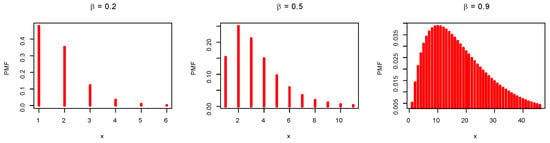
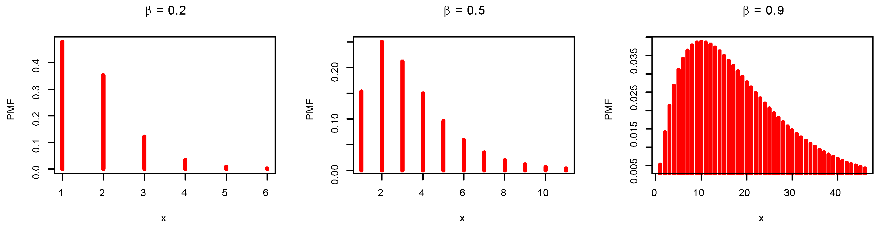
respectively, where controls the shape of the distribution. Figure 1 shows the PMF plots for various values of the parameter .
Figure 1.
PMF visualization plots for the DMEx model.
As can be seen, the PMF is unimodally shaped, and it can be applied to discuss the positively skewed count data. The HRF can be proposed as
The reversed hazard rate function (RHRF) is given by
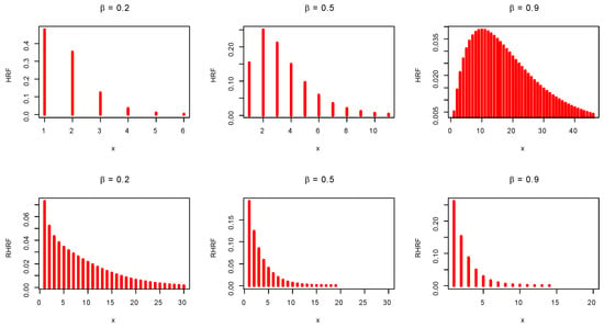
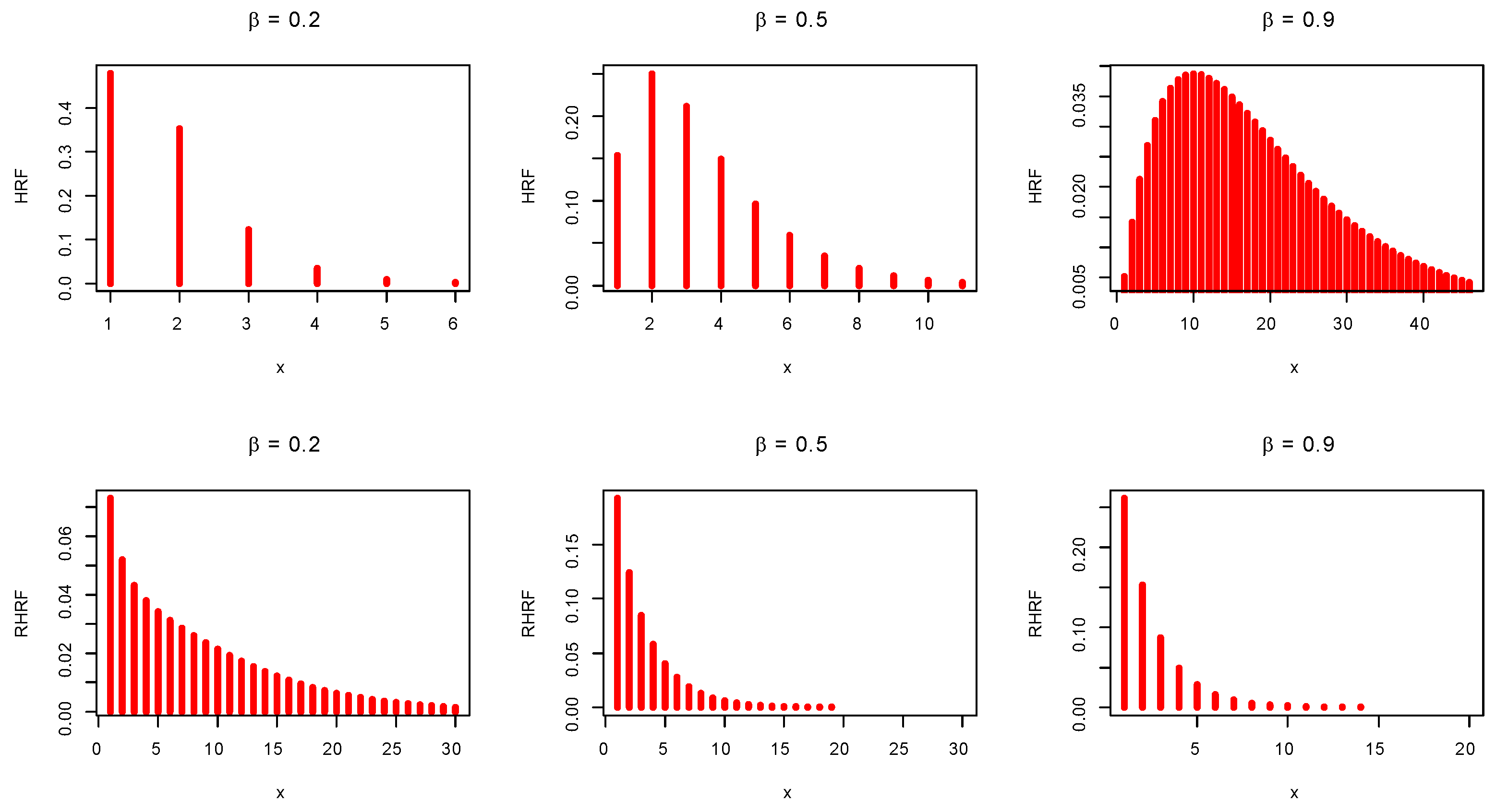
Figure 2 shows the HRF and RHRF plots for different values of the distribution parameter .
Figure 2.
HRF and RHRF visualization plots for the DMEx model.
Both the HRF and its reversed function can be used effectively to model decreasing or unimodal failure modes.
2.1. Moments of a Statistical Distribution
Assume X is a DMEx RV, the probability generating function (PGF), say , can be derived in a closed form as
where the power series converges at least for all complex numbers s with . Equation (8) can be derived utilizing the Maple software program. Thus, the first four moments of the DMEx distribution can be expressed as
and
Using Equations (9)–(12), the , , and can be derived in closed forms where
and
The moment generating function (MGF) can be expressed as
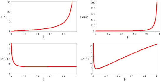
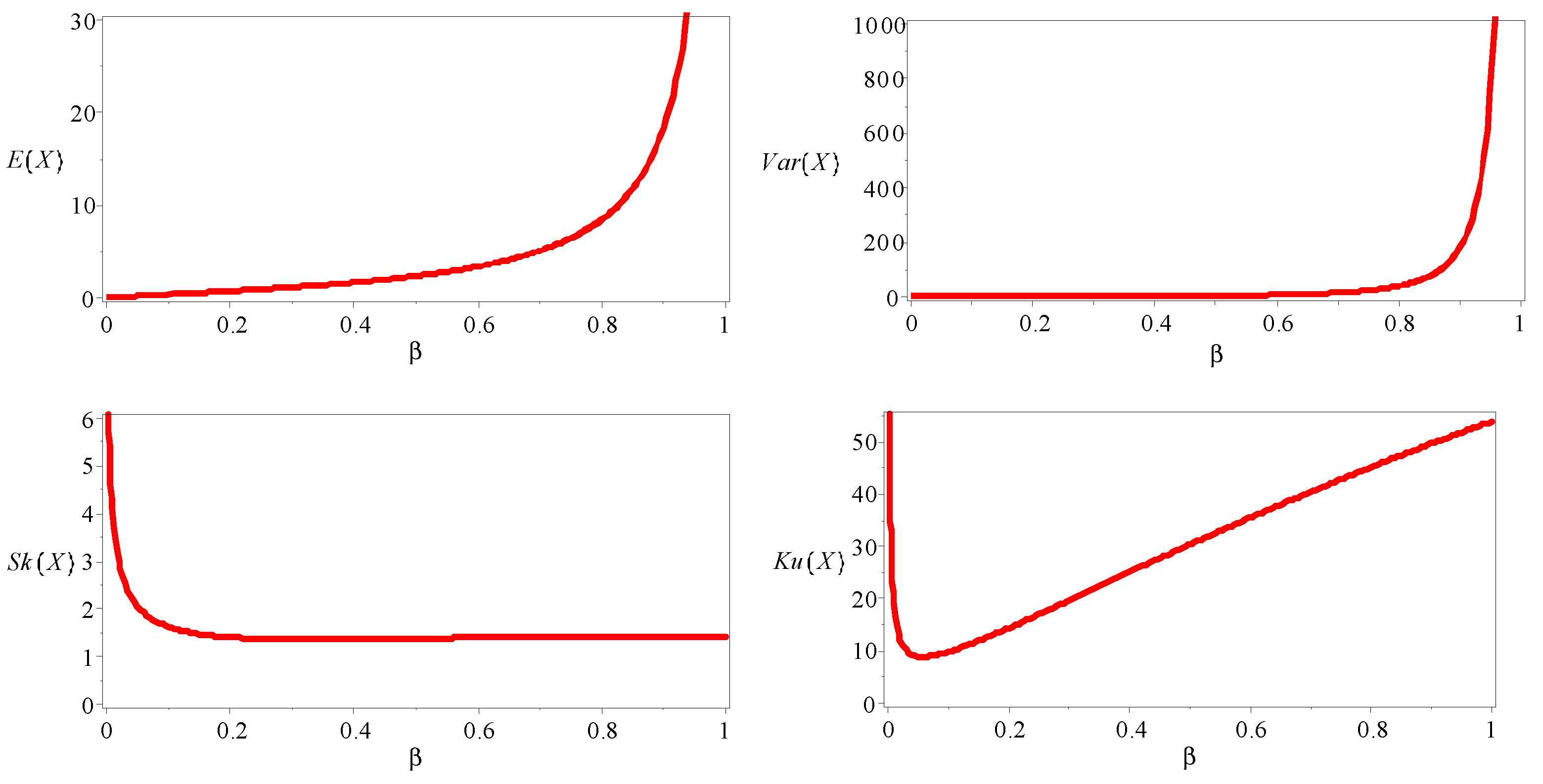
Table 1 lists some computational statistics (CS) of the DMEx model based on various values of the parameter . All results given in Table 1 are reported in Figure 3.
Table 1.
Some CS of the DMEx distribution.
Figure 3.
The plots of descriptive measures of the DMEx distribution.
As can be seen, both the and of the DMEx distribution increase when grows to one. Further, the DMEx model is capable of modeling positively skewed count data under a leptokurtic shape.
2.2. Dispersion and Variation Measures
The index of dispersion, say , is related to the coefficient of variation, say . The is also referred to as the coefficient of dispersion, which can be utilized to decide the possible over “” or under “” dispersion in the used data set. The measure is generally applied for comparison with independent samples based on their variability. A higher value indicates a higher variability. Let X be a DMEx RV. Then, the and can be formulated as
and
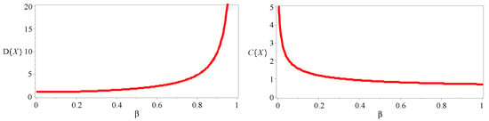
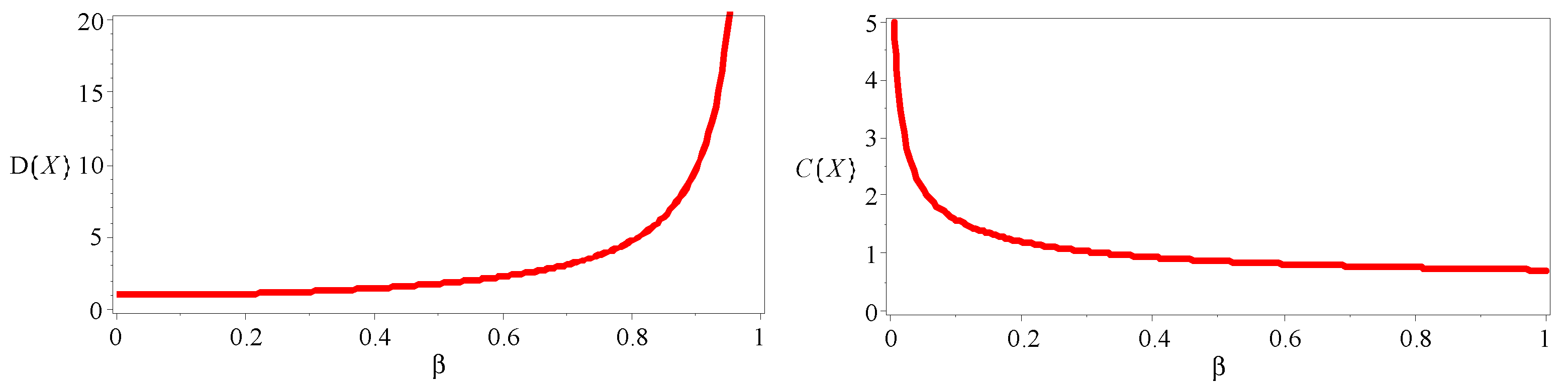
respectively, where and . Table 2 shows some numerical calculations for and of the DMEx model based on the different values of the parameter . All results given in Table 2 are reported in Figure 4.
Table 2.
The and statistics of the DMEx distribution.
Figure 4.
Plots of the and statistics of the DMEx distribution.
As can be seen, for , the of the DMEx distribution increases whereas the decreases. Moreover, the DMEx model is appropriate for modeling over- and under-dispersed count data.
2.3. L-Moment Statistics
Suppose that n random variables are ordered in non-decreasing magnitude and written as In the definition of order statistics (OS), there is no restriction on whether s are independent or identically distributed (IID); however, many well-known results about OS are under the classical assumption that s are IID. Let the RV X have the DMEx distribution. Then, the CDF of the ith OS can be expressed as
where . Furthermore, the corresponding PMF of the ith OS can be proposed as
Thus, the rth moments of , say , can be expressed as
The L-moments (L-M), say , are summary statistics for probability models. They are analogous to ordinary moments but are computed from linear functions of the ordered data values. The L-M of the RV X can be proposed as
Using Equation (19), some statistical measures based on the L-M statistics can be computed, such as , and .
3. Different Estimation Techniques
3.1. Maximum Likelihood Estimation (MLE)
In this subsection, estimation of the DMEx parameter is discussed using the method of maximum likelihood based on a complete sample. Let be a random sample (RS) from a DMEx distribution. Then, the log-likelihood, say L, a function of the DMEx may be expressed as
Differentiating Equation (20) with respect to the parameter and setting the result equal to 0, we obtain
Since Equation (21) cannot be derived in the closed form as a function of only the data “”, a numerical iterative procedure is required to solve it numerically “Newton-Raphson as an example”.
3.2. Moment Estimation (ME)
Using the moment approach to estimate , we must first equate the population moment to the corresponding sample moment and then solve the non-linear equation
with respect to
3.3. Proportion Estimation (PE)
Let , , …, be an RS from the DMEx distribution. Since we have one unknown parameter, one indicator function is defined as follows
Assume denotes the number of zeroes in the sample. Using Equations (4) and (23), we obtain . Hence, we obtain the estimation of the parameter by solving the following equation
Since is an unbiased and consistent empirical estimator of probability , the is also an unbiased and consistent estimator of
4. Comparing Different Estimators (CDEs): A Simulation Study
In this segment, we assess the performance of the MLE, ME, and PE with respect to the sample size n utilizing R software. For CDEs, MCMC simulations are performed according to different schemes. The assessment is according to a simulation study:
- 1.
- Generate samples of various sizes “” from the DMEx model as follows
- Scheme I: |
- Scheme II: |
- Scheme III: |
- 2.
- Compute the MLE, ME, and PE for the 10,000 samples, say for 10,000.
- 3.
- Calculate the bias “BS”, mean squared errors (MSE), and mean relative errors (MRE) for N = 10,000 samples as
- 4.
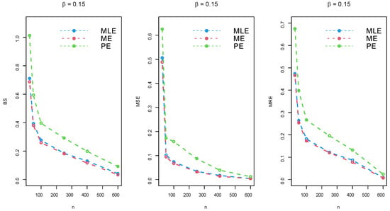
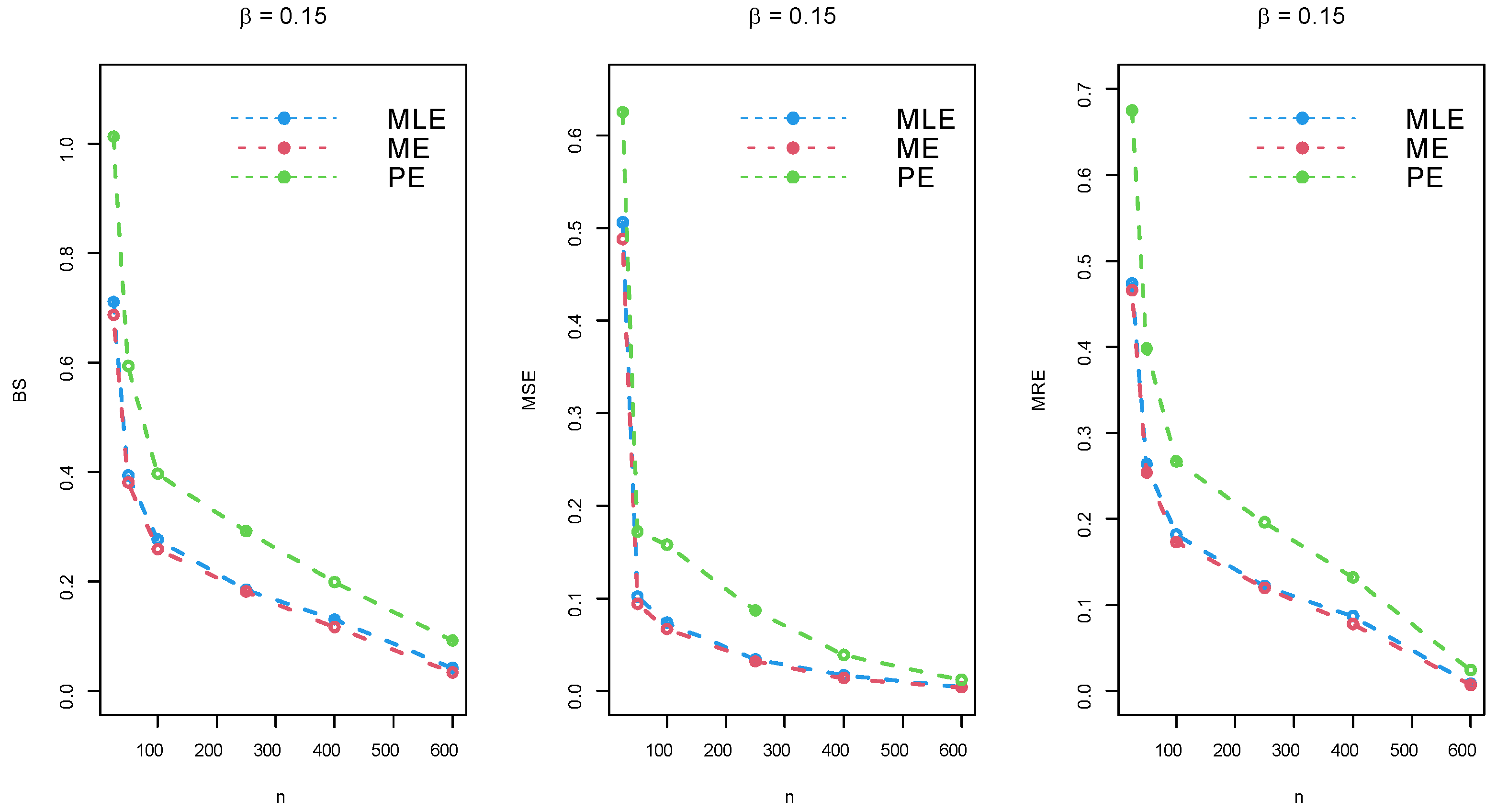
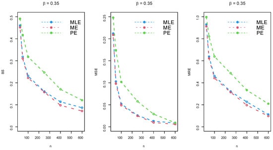
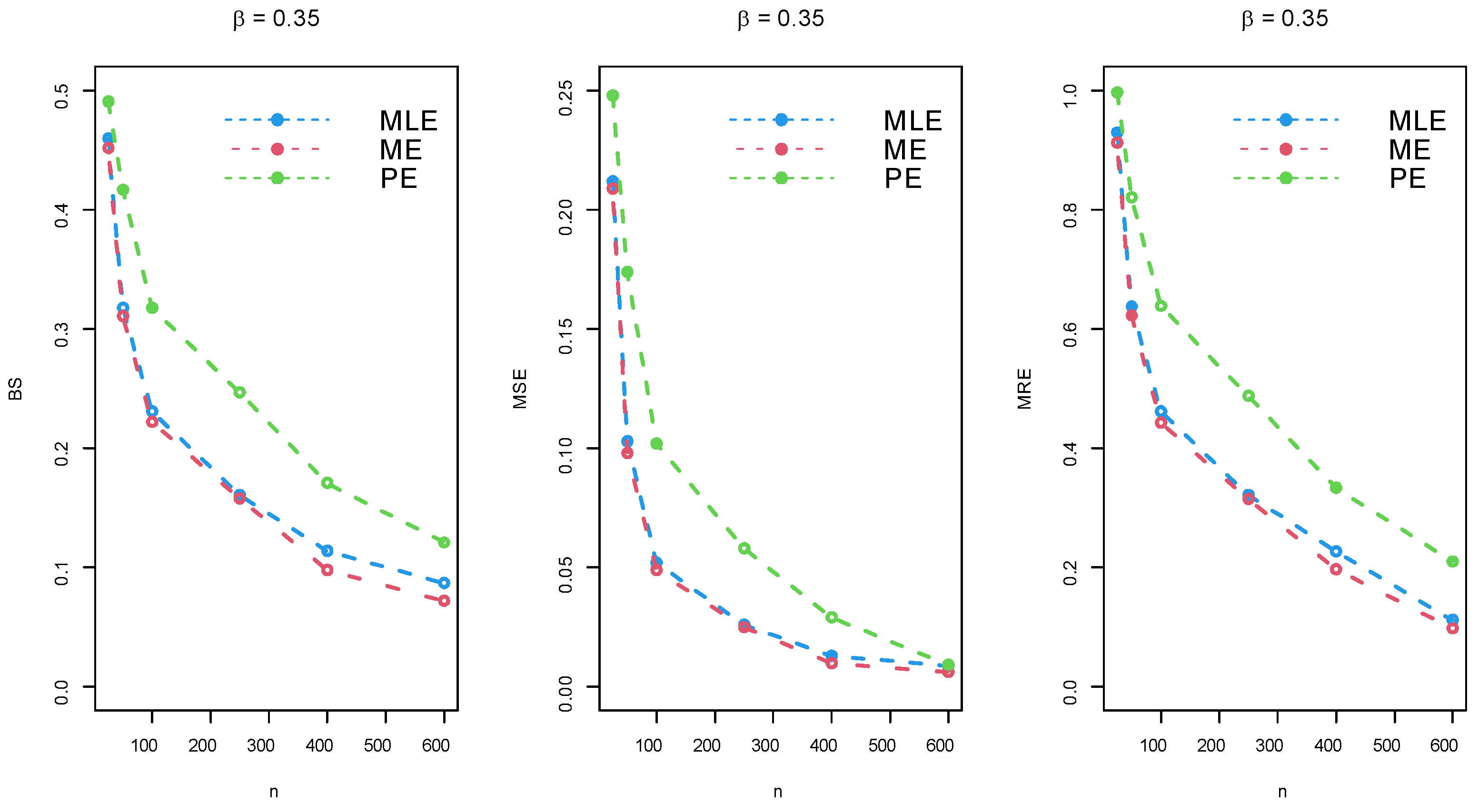
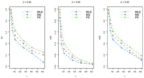
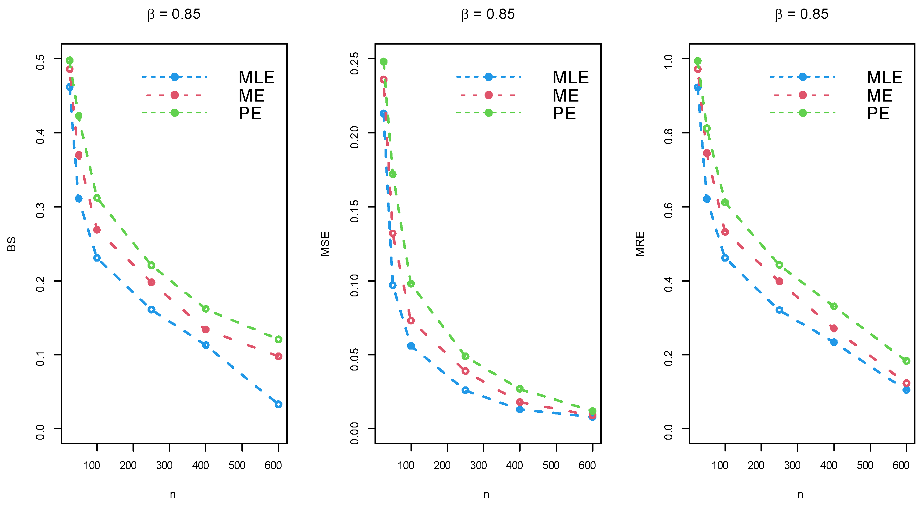
- The empirical results of the simulations are reported in Table 3, Table 4 and Table 5 and provided via Figure 5, Figure 6 and Figure 7.Table 3. Simulation results for = 0.15.Table 4. Simulation results for = 0.35.Table 5. Simulation results for = 0.85.Figure 5. Simulation for .Figure 6. Simulation for .Figure 7. Simulation .
As can be seen, the BS of the parameter approaches 0 when the sample size n grows. Similarly, both the MSE and MRE of the DMEx parameter approach 0 when the sample size n increases. These results reveal the consistency property of the derived estimators. Thus, we can conclude that all estimation methods work quite well under various sizes of samples.
5. Data Modeling: Competitive Models and Statistical Criteria
In this segment, the importance of the DMEx distribution is discussed utilizing data sets from various areas. We shall compare the fits of the DMEx model with diverse competitive distributions, such as the Poisson (Poi), the discrete Pareto (DPa), the discrete Burr-XII (DBXII), the discrete Rayleigh (DR), the discrete Burr–Hatke (DBH), and the discrete inverse Rayleigh (DIR) models. The tested distributions are compared to some criteria, such as , the Hannan–Quinn information criterion (HQIC), the Akaike information criterion (AIC), the Bayesian information criterion (BIC), the corrected AIC (CAIC), and the Kolmogorov–Smirnov (KS) test with its p-value.
5.1. Data Set I: Electronic Components
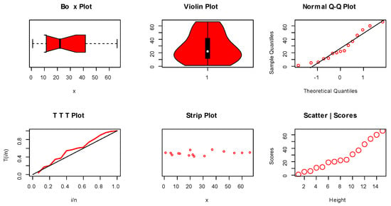
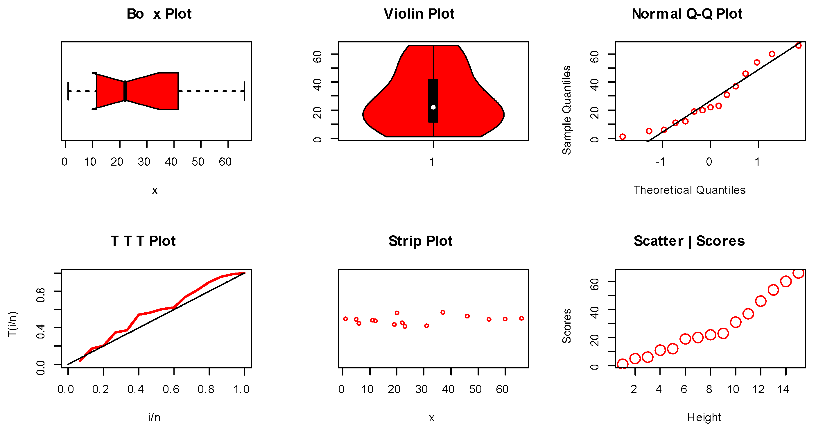
The first set of data represents the failure times for a sample of 15 electronic components (EC) in an accelerated life test (see, Johnston [17]). The observed descriptive statistics (ODS) include: mean = 27.533, variance = 631.980, skewness = 1.534, and kurtosis = 6.924. Non-parametric plots for the EC data are sketched in Figure 8.
Figure 8.
Non-parametric visualization plots for EC data.
The MLE with their SE, the CI for the parameter(s), and the goodness of fit (GOF) test for these data are reported in Table 6 and Table 7.
Table 6.
The MLE, SE, and CI for EC data.
Table 7.
The GOF test for EC data.
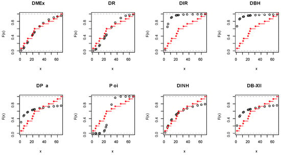
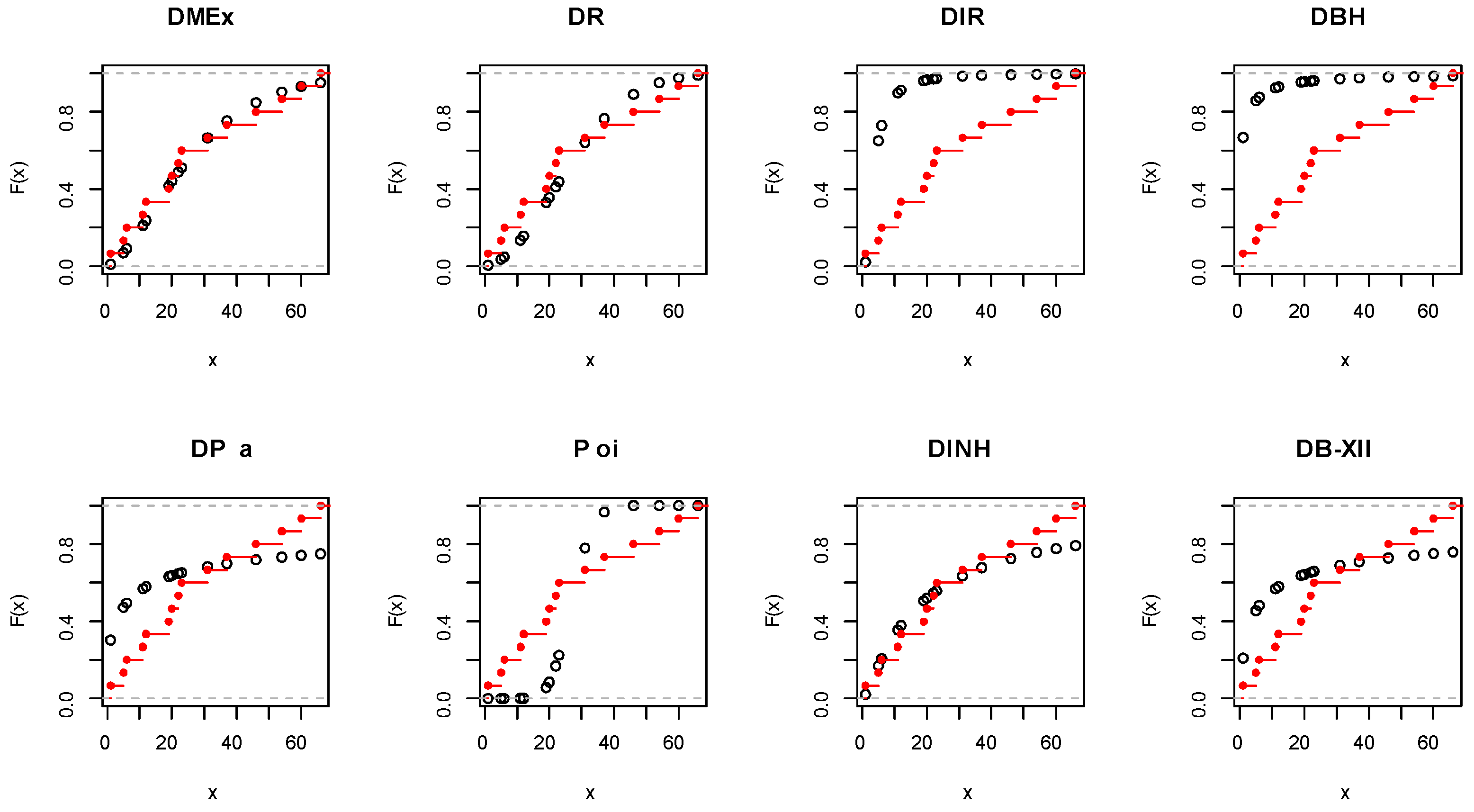
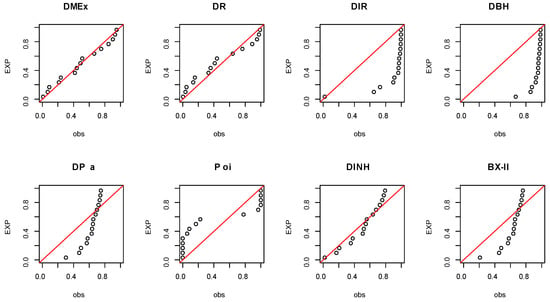
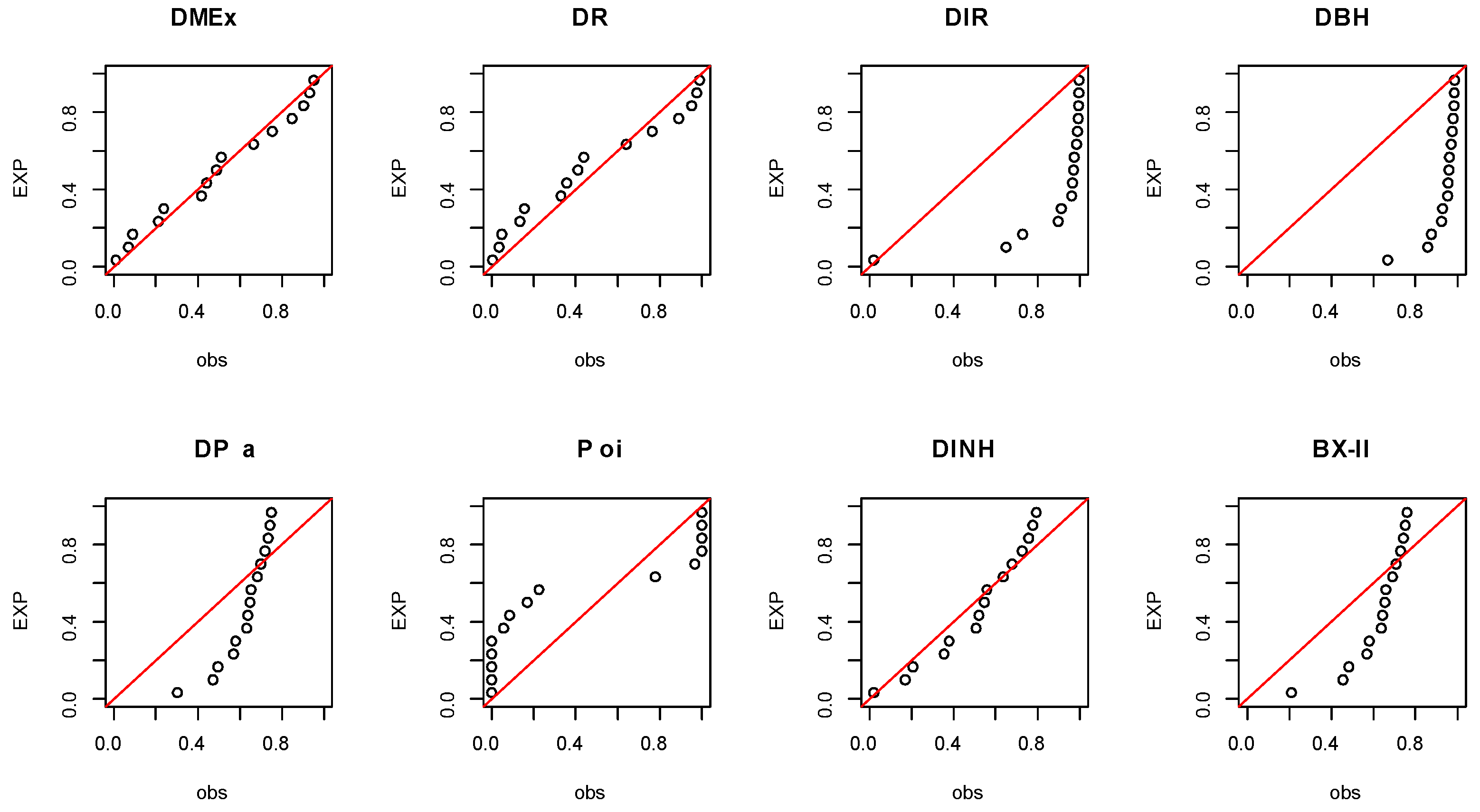
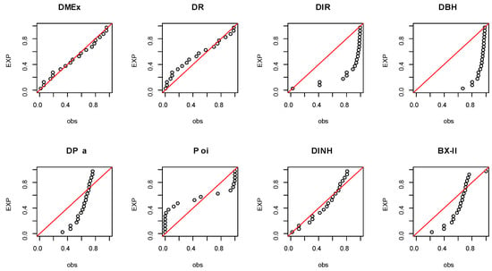
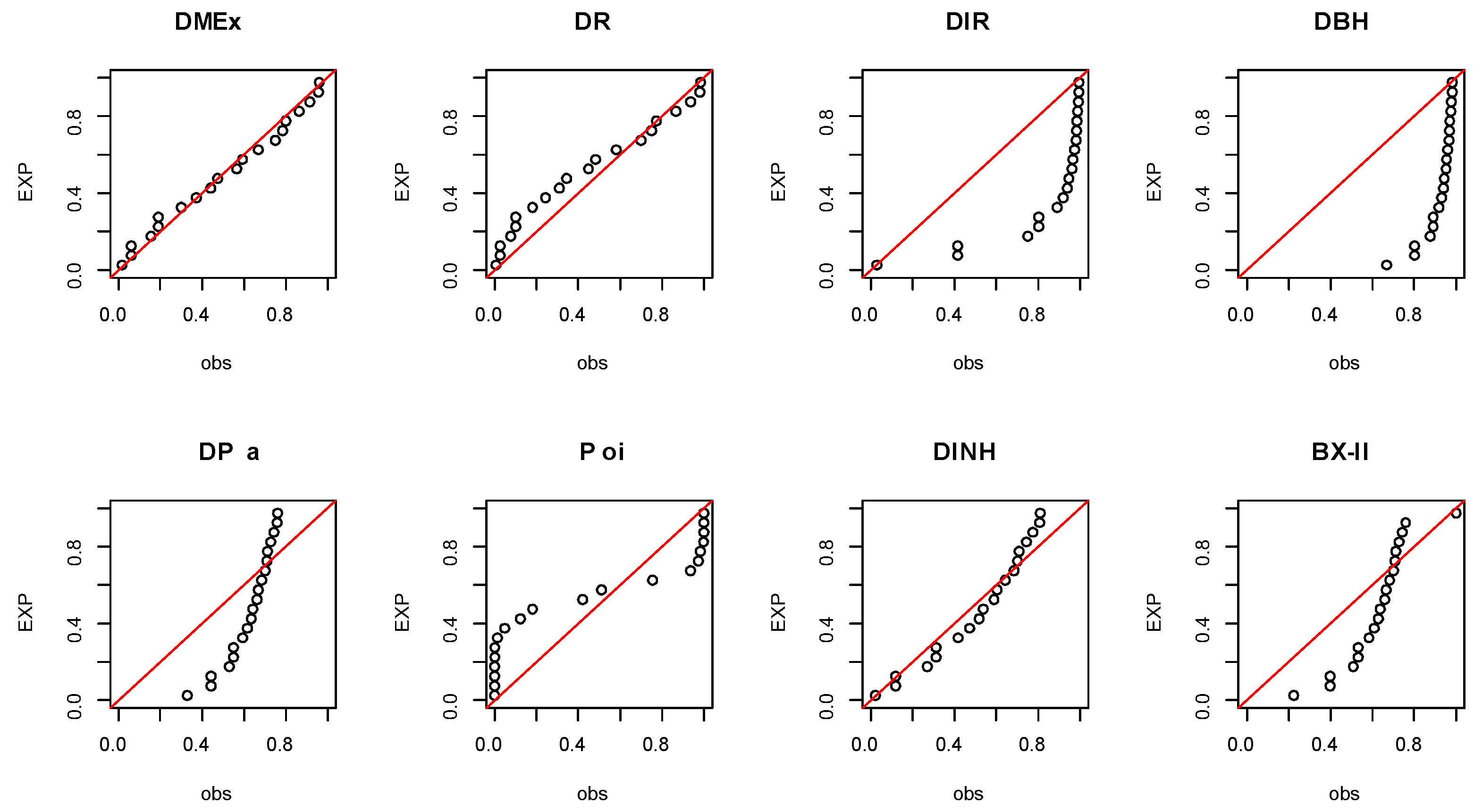
As can be noted, based on a significance level of , both the DMEx and DR models work quite well for modeling the EC data, but the DMEx distribution is the best. Figure 9 and Figure 10 show the empirical CDFs as well as the probability-probability (P-P) plots, or “parametric plots”, for the EC data, which prove the empirical results mentioned in Table 7.
Figure 9.
Empirical CDF visualization plots for EC data.
Figure 10.
P-P visualization plots for EC data.
Table 8 lists various estimators for the EC data, and it is noted that the MLE and ME techniques work quite well for modeling these data.
Table 8.
Different estimators for EC data.
Table 9 reports some numerical accounts of the empirical descriptive statistics (EDS).
Table 9.
The EDS for EC data.
Both theoretical and empirical “MLE and ME” scales are approximately equal. Thus, the ME approach works quite well beside the MLE method for estimating the unknown parameter. The performance of the PE approach is inferior compared to other techniques for some measures. The EC data are suffering from over-dispersed phenomena. Moreover, the EC data are skewed to the right and leptokurtic.
5.2. Data Set II: Leukemia Remission
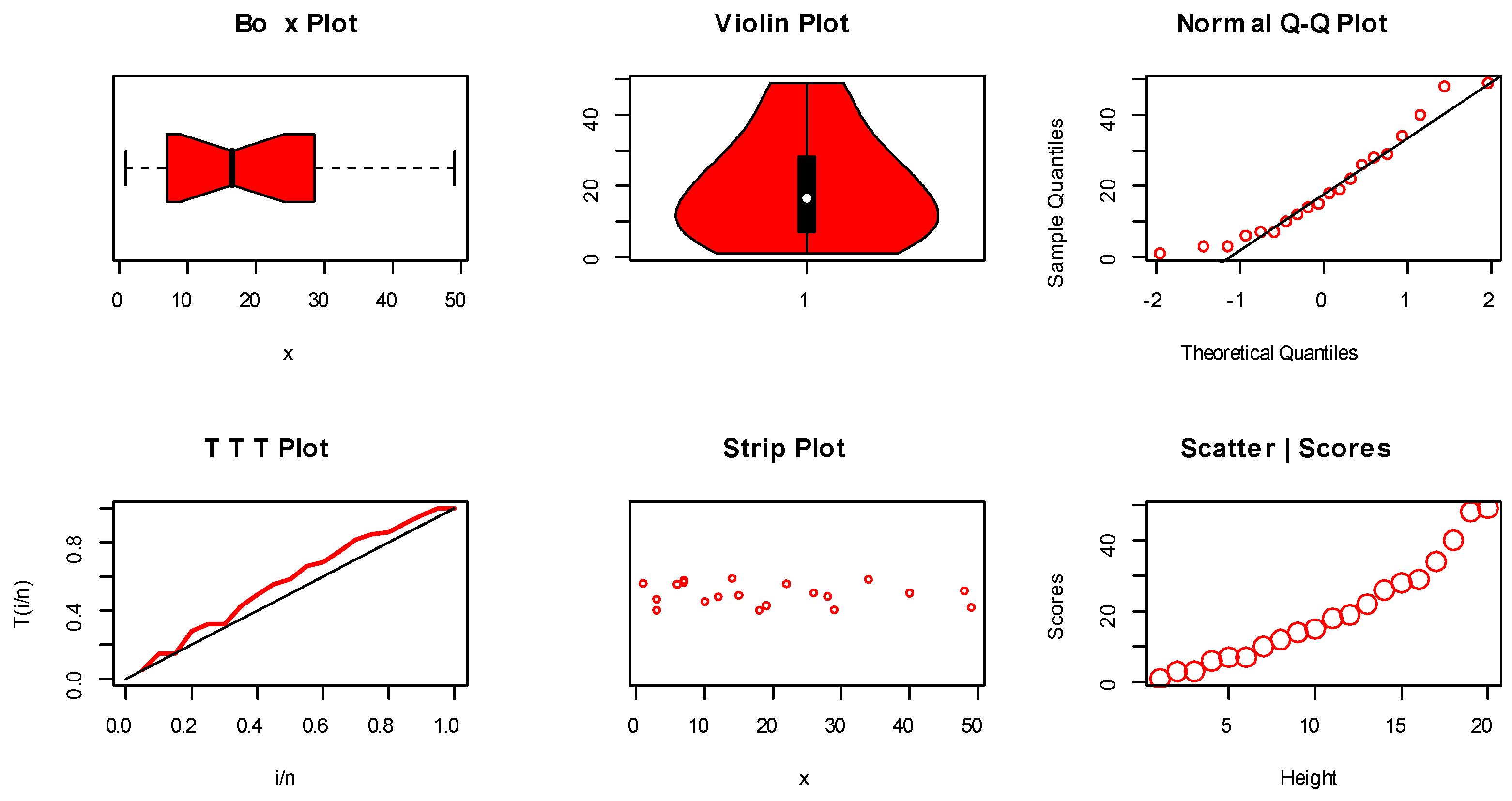
These data involve leukemia remission (LR) times (in weeks) for 20 patients (see Damien and Walker [18]) according to the discretization concept. For these data, the ODS equals , , , and . Non-parametric plots for the LR data are displayed in Figure 11.
Figure 11.
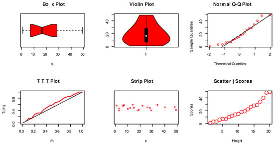
Non-parametric visualization plots for LR data.
The MLE with their SE, the CI for the parameter(s), and the GOF test for the LR data are listed in Table 10 and Table 11.
Table 10.
The MLE, SE, and CI for LR data.
Table 11.
The GOF test for LR data.
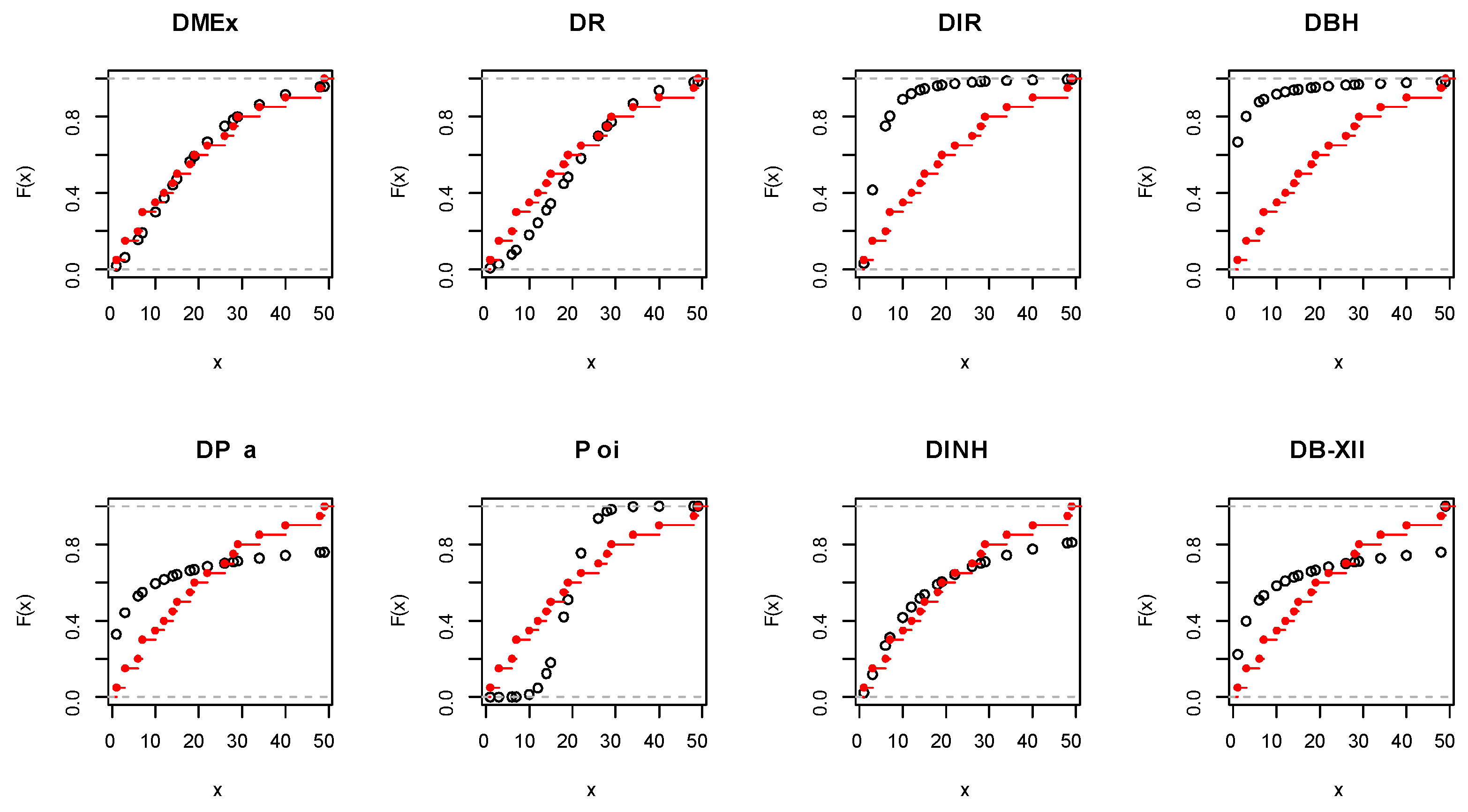
Based on a significance level of , both the DMEx and DR distributions work quite well for analyzing the LR data, but the DMEx model is the best. Figure 12 and Figure 13 show the empirical CDFs as well as the P-P plots for the LR data, which prove the empirical results reported in Table 11.
Figure 12.
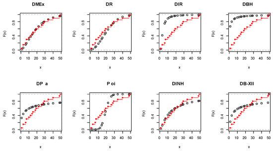
Empirical CDF visualization plots for LR data.
Figure 13.
P-P visualization plots for LR data.
Table 12 reports different estimators for the LR data, and it is noted that the MLE and ME methods work quite well for modeling these data.
Table 12.
Different estimators for LR data.
Table 13 lists some numerical accounts of the EDS for the LR data.
Table 13.
The EDS for LR data.
The ME approach works quite well beside the MLE technique for estimating the unknown parameter. The LR data are suffering from over-dispersed phenomena. Further, the LR data are skewed to the right and leptokurtic.
5.3. Data Set III: Coronavirus in Punjab
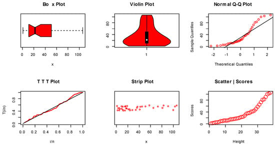
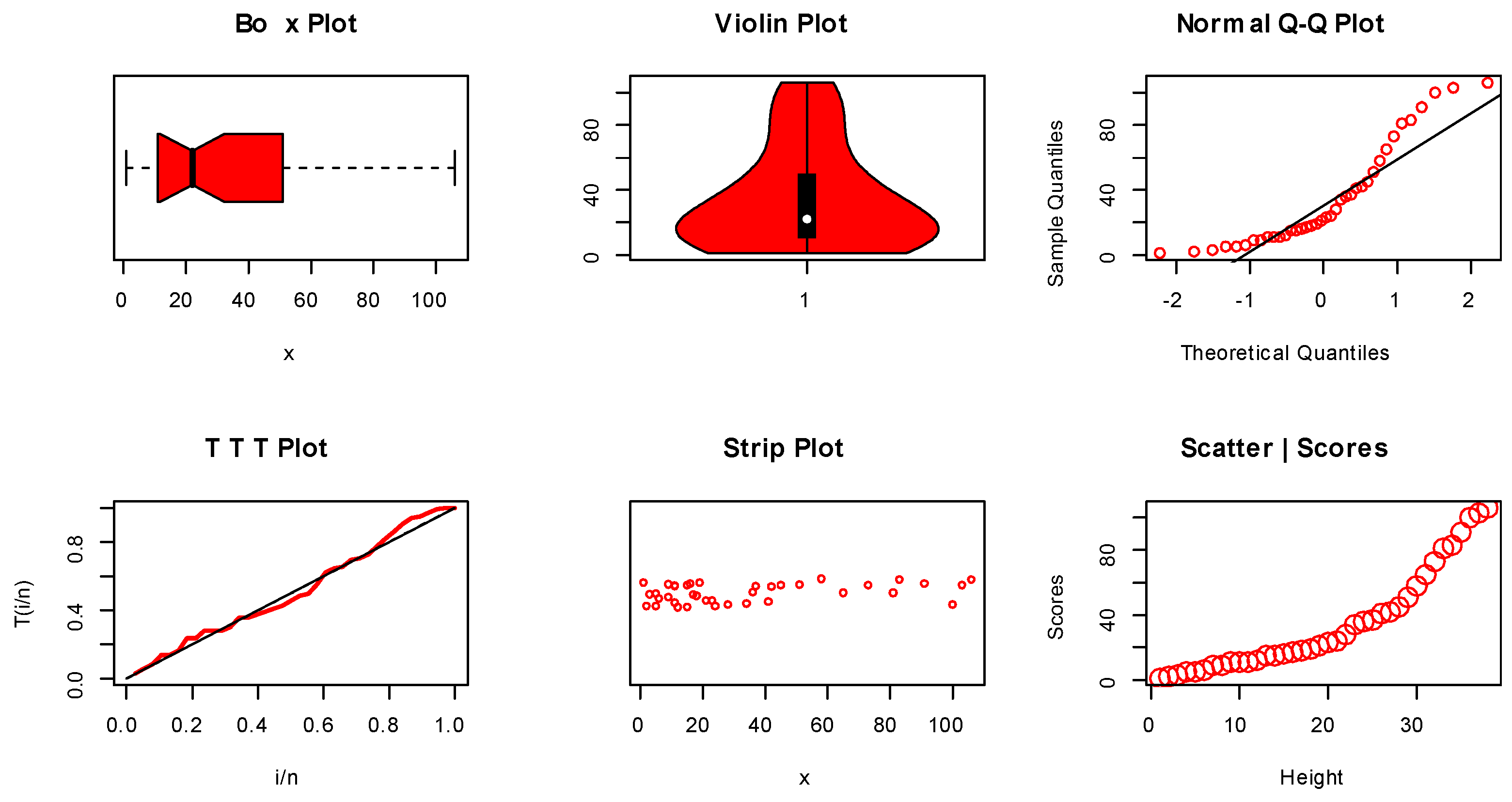
The third set of data represents the number of deaths due to coronavirus in Punjab (COV-P) during the period from 24 March 2020 to 30 April 2020. The data are as follows: 1, 2, 3, 5, 5, 6, 9, 9, 11, 11, 11, 12, 15, 15, 16, 17, 18, 19, 21, 23, 24, 28, 34, 36, 37, 41, 42, 45, 51, 58, 65, 73, 81, 83, 91, 100, 103, 106. Non-parametric plots for the COV-P data are listed in Figure 14.
Figure 14.
Non-parametric visualization plots for COV-P data.
The MLE with their SE, the CI for the parameter(s), and the GOF test for the COV-P data are proposed in Table 14 and Table 15.
Table 14.
The MLE, SE, and CI for COV-P data.
Table 15.
The GOF test for COV-P data.
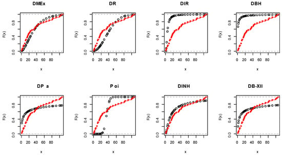
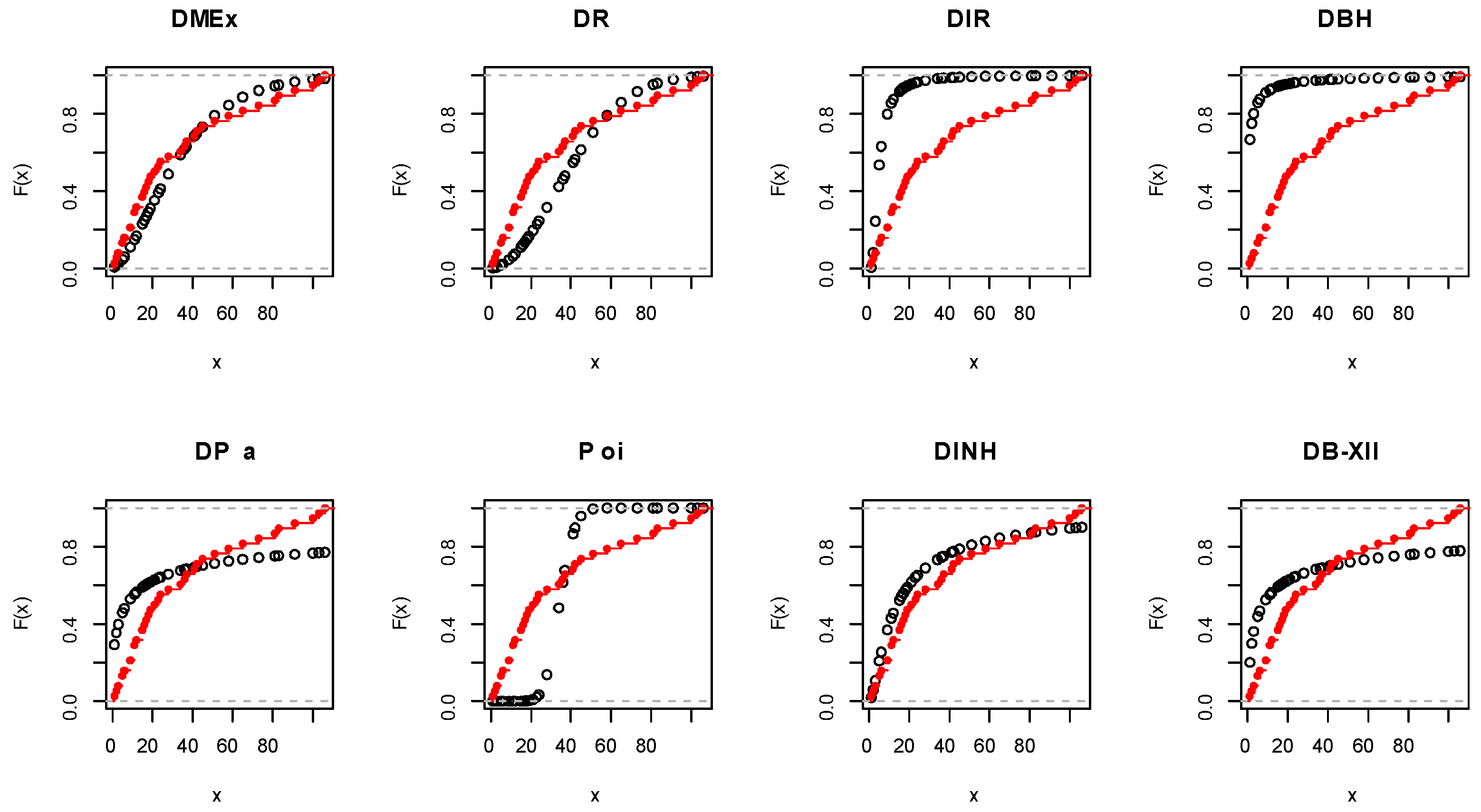
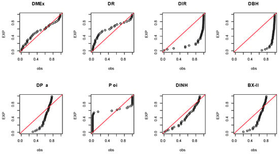
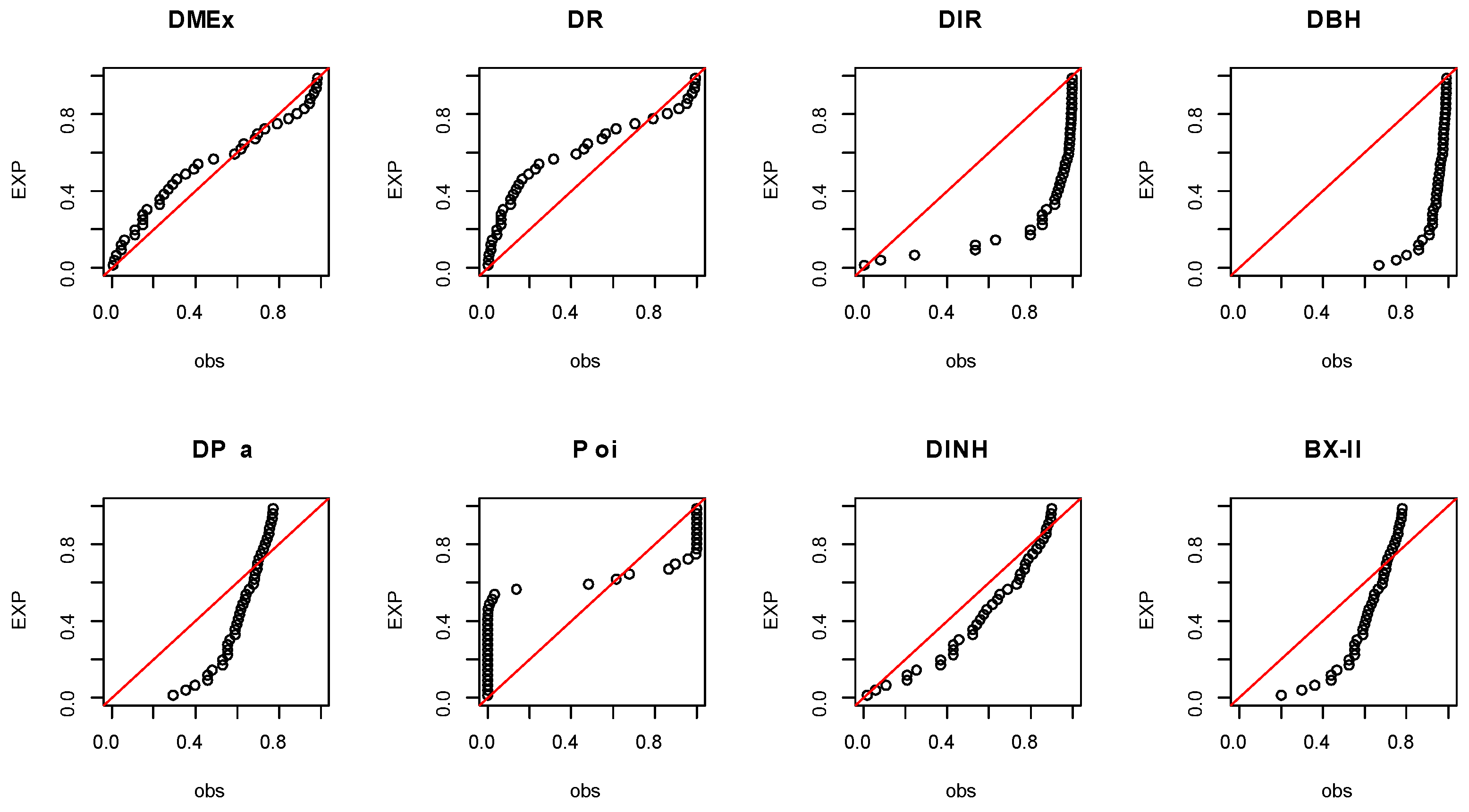
Based on a significance level of , the DMEx distribution is the best among all tested models. Figure 15 and Figure 16 show the empirical CDFs as well as the P-P plots for the COV-P data, which prove the empirical results listed in Table 15.
Figure 15.
Empirical CDF visualization plots for COV-P data.
Figure 16.
P-P visualization plots for COV-P data.
Table 16 reports various estimators for the COV-P data, and it is noted that the MLE and ME techniques work quite well for discussing these data.
Table 16.
Different estimators for COV-P data.
Table 17 introduces some numerical accounts of the EDS for the COV-P data.
Table 17.
The EDS for COV-P data.
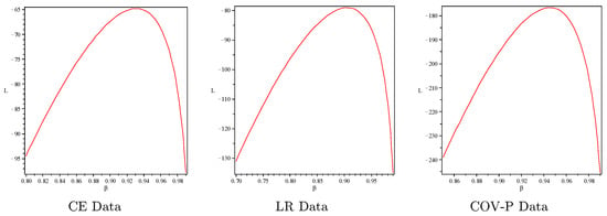
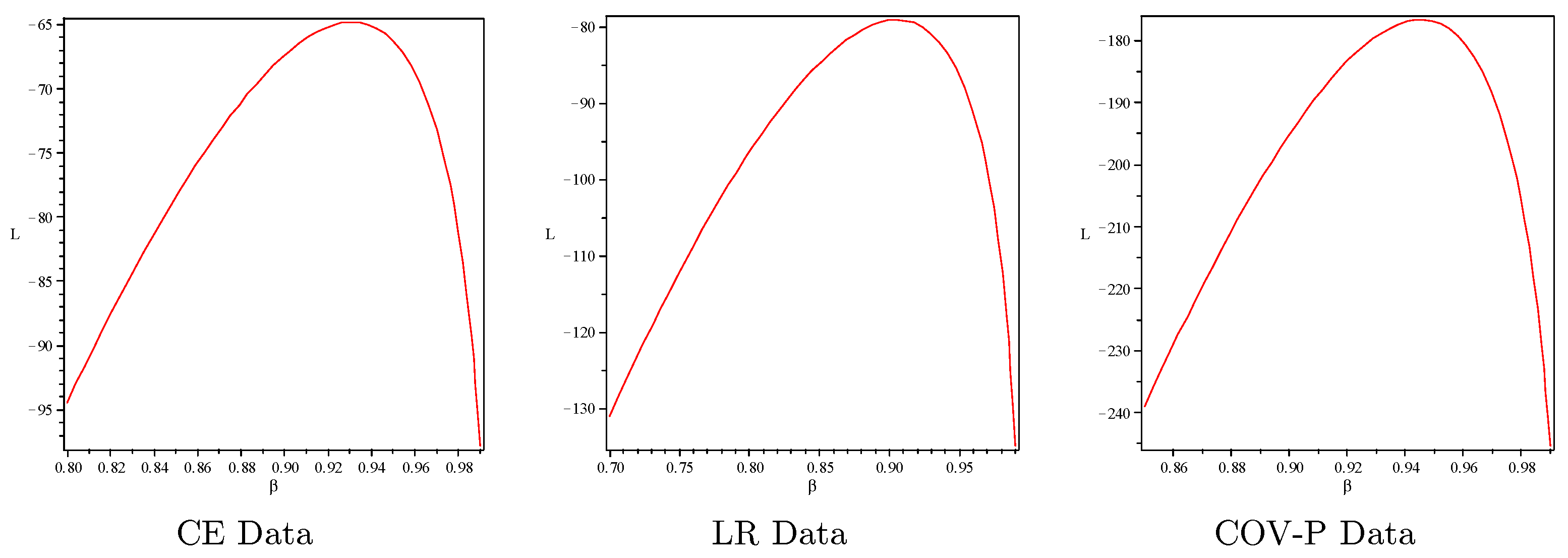
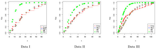
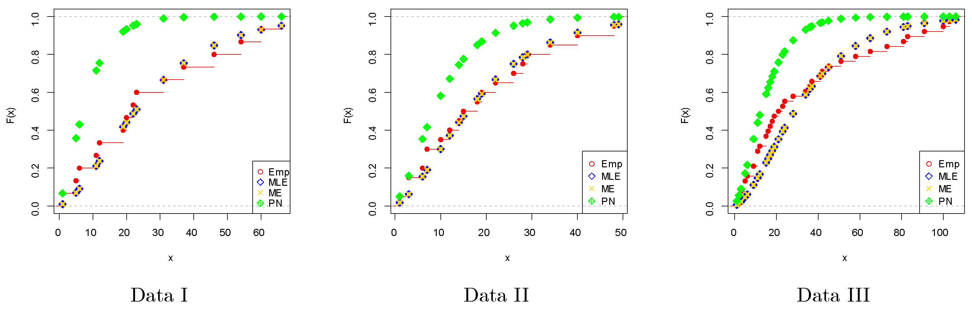
The ME approach works quite well beside the MLE technique for estimating the unknown parameter. The COV-P data are suffering from over-dispersed phenomena. Moreover, the COV-P data are skewed to the right and leptokurtic. The profiles of the L functions for data sets I, II, and III are displayed in Figure 17, and it is noted that the estimator is a unique “unimodal function”. Figure 18 shows the empirical CDFs for the different estimation approaches.
Figure 17.
The profiles plots of L for data sets.
Figure 18.
Empirical CDF visualization plots for different estimation methods.
6. Concluding Remarks and Future Work
This article focuses on a one-parameter discrete distribution created based on the survival discretization approach and called the DMEx distribution. The statistical properties of the DMEx model have been derived and expressed in closed forms. It was found that the DMEx model is proper for modeling right-skewed data sets of a leptokurtic shape. The presented discrete distribution can be used as a statistical tool to model different types of HRFs, including those that are decreasing and unimodally shaped. The DMEx parameter has been estimated utilizing various estimation approaches, i.e., MLE, ME, and PE. Simulation studies have been performed based on various sample sizes, and it was found that the MLE and ME techniques work quite effectively for estimating the DMEx parameter. Finally, three real data sets have been analyzed and discussed to illustrate the notability of the DMEx distribution, and it was found that DMEx outperforms all other competitive distributions in all aspects of the current study. In the future, the bivariate extension of the DMEx models will be proposed and discussed in detail. Furthermore, a regression model and INAR(1) process will be discussed alongside their applications.
Author Contributions
Conceptualization, M.S.E.; data curation, M.E.-M. and H.S.S.; formal analysis, M.S.E. and B.A.; investigation, M.E.-M. and H.S.S.; methodology, M.E.-M. and M.S.E.; resources, H.S.S. and B.A.; software, M.E.-M., H.S.S. and M.S.E.; validation, M.S.E. and B.A.; writing— review and editing, M.S.E. All authors have read and agreed to the published version of the manuscript.
Funding
Project number (IF-PSAU-2022/01/22553).
Data Availability Statement
All data sets have been listed within the paper.
Acknowledgments
The authors extend their appreciation to the Deputyship for Research & Innovation of the Ministry of Education in Saudi Arabia for funding this research work through project number (IF-PSAU-2022/01/22553).
Conflicts of Interest
The authors declare no conflict of interest.
References
- Bhatti, F.A.; Hamedani, G.G.; Korkmaz, M.Ç.; Sheng, W.; Ali, A. On the Burr XII-moment exponential distribution. PLoS ONE 2021, 16, e0246935. [Google Scholar] [CrossRef] [Scilit] [PubMed]
- Iqbal, Z.; Hasnain, S.A.; Salman, M.; Ahmad, M.; Hamedani, G. Generalized exponentiated moment exponential distribution. Pak. J. Stat. 2014, 30, 537–554. [Google Scholar]
- Ahsan-ul-Haq, M. On Poisson moment exponential distribution with applications. Ann. Data Sci. 2022, 1–22. [Google Scholar] [CrossRef] [Scilit]
- Abbas, S.; Jahngeer, A.; Shahbaz, S.H.; Afify, A.Z. Topp-Leone moment exponential distribution: Properties and applications. 2020. J. Natl. Sci. Found. Sri Lanka 2020, 48, 265–274. [Google Scholar] [CrossRef] [Scilit]
- Akhter, Z.; MirMostafaee, S.M.T.K.; Ormoz, E. On the order statistics of exponentiated moment exponential distribution and associated inference. J. Stat. Comput. Simul. 2022, 92, 1322–1346. [Google Scholar] [CrossRef] [Scilit]
- Hashmi, S.; Haq, M.A.U.; Usman, R.M.; Ozel, G. The Weibull-moment exponential distribution: Properties, characterizations and applications. J. Reliab. Stat. Stud. 2019, 12, 1–22. [Google Scholar]
- Kumar, D.; Dey, T.; Dey, S. Statistical inference of exponentiated moment exponential distribution based on lower record values. Commun. Math. Stat. 2017, 5, 231–260. [Google Scholar] [CrossRef] [Scilit]
- Iriarte, Y.A.; Astorga, J.M.; Venegas, O.; Gómez, H.W. Slashed moment exponential distribution. J. Stat. Appl. 2017, 16, 354–365. [Google Scholar] [CrossRef] [Scilit]
- Ibrahim, M.; Ali, M.M.; Yousof, H.M. The discrete analogue of the Weibull-G family: Properties, different applications, Bayesian and non-Bayesian estimation methods. Ann. Data Sci. 2021, 1–38. [Google Scholar] [CrossRef] [Scilit]
- Eliwa, M.S.; El-Morshedy, M.; Yousof, H.M. A discrete exponential generalized-G family of distributions: Properties with Bayesian and non-Bayesian estimators to model medical, engineering and agriculture data. Mathematics 2022, 10, 3348. [Google Scholar] [CrossRef] [Scilit]
- Yousof, H.M.; Chesneau, C.; Hamedani, G.; Ibrahim, M. A new discrete distribution: Properties, characterizations, modeling real count data, Bayesian and non-Bayesian estimations. Statistica 2021, 81, 135–162. [Google Scholar] [CrossRef]
- Altun, E.; El-Morshedy, M.; Eliwa, M.S. A study on discrete Bilal distribution with properties and applications on integervalued autoregressive process. Revstat-Stat. J. 2022, 20, 501–528. [Google Scholar]
- El-Morshedy, M.; Altun, E.; Eliwa, M.S. A new statistical approach to model the counts of novel coronavirus cases. Math. Sci. 2022, 16, 37–50. [Google Scholar] [CrossRef] [Scilit] [PubMed]
- Almetwally, E.M.; Ibrahim, G.M. Discrete alpha power inverse Lomax distribution with application of COVID-19 data. J. Appl. Math. 2020, 9, 11–22. [Google Scholar]
- Tyagi, A.; Choudhary, N.; Singh, B. A new discrete distribution: Theory and applications to discrete failure lifetime and count data. J. Appl. Probab. Stat. 2020, 15, 117–143. [Google Scholar]
- Bakouch, H.S.; Jazi, M.A.; Nadarajah, S. A new discrete distribution. Statistics 2014, 48, 200–240. [Google Scholar] [CrossRef] [Scilit]
- Johnston, G. Statistical Models and Methods for Lifetime Data; Wiley: New York, NY, USA, 2003. [Google Scholar]
- Damien, P.; Walker, S. A Bayesian non-parametric comparison of two treatments. Scand. J. Stat. 2002, 29, 51–56. [Google Scholar] [CrossRef] [Scilit]

Publisher’s Note: MDPI stays neutral with regard to jurisdictional claims in published maps and institutional affiliations. |
© 2022 by the authors. Licensee MDPI, Basel, Switzerland. This article is an open access article distributed under the terms and conditions of the Creative Commons Attribution (CC BY) license (https://creativecommons.org/licenses/by/4.0/).