Regularization Cuckoo Search Algorithm for Multi-Parameter Optimization of the Multi-Laminated Controlled Release System

Abstract

The multi-laminated controlled release system has been widely used in the modern pharmaceutical industry because of its simple structure and safety, which can control the drug release behavior by regulating its internal parameters. To achieve three desired drug release behaviors of constant rate, linear reduction, and nonlinearity, which can be controlled by the optimization of the controllable parameters in the controlled release system, such as initial concentration and diffusion coefficient, a new regularization cuckoo search algorithm based on the cuckoo search algorithm and Tikhonov regularization method is proposed. The numerical examples confirm the stability, effectiveness, and feasibility of the proposed method. The effect of the number of model layers on the optimization results is also analyzed.

1. Introduction

A controlled release system can control the concentration of the target substance in the release environment by regulating the release rate of the substance into the environment. This technology was firstly applied in agriculture for pesticides, fertilizers, herbicides, and other substances that require controlled release [1]. With the development of controlled release technology in recent years, it has been widely used in many fields such as drug delivery, hygiene and disinfection, mold prevention, and odor control because of its safe and reliable properties [2,3]. Especially in the field of drug delivery, controlled release technology has been developed rapidly and has a broad development prospect. It has been found that the drug release behavior is generally characterized by a sudden release followed by a first-order kinetic release. The sudden release refers to the high release rate at the beginning of the release, and then the release rate becomes rapidly decreased due to the decrease of drug concentration in the transport matrix. Sudden release behavior will bring serious drug side effects. It is also found that the drug release rate can be controlled by optimizing the initial concentration, diffusion coefficient, and the number of model layers of multi-laminated drug-controlled release system so as to overcome the hazards and drug wastage caused by the sudden release behavior and achieve different drug release behaviors.

At present, for multi-laminated drug-controlled release systems, most investigations have been conducted on the mechanism of the controlled release system, while relatively little work has been done to study the drug release behavior. In 1998, Lu et al. [4] designed a multi-laminated system for drug release and obtained an inhomogeneous initial drug concentration distribution to achieve the desired release rate; in 2001, Georgiadis and Kostoglou [5] proposed a framework for controlled parameter optimization using an analytical solution-based optimization method and a dynamic optimization method to optimize the design of multiple parameters to make the constant rate release behavior as expected; in 2010, Nauman et al. [6] optimized the initial drug concentration distribution of the controlled release system by a stochastic search method to achieve constant release; in 2014, Huang and Wang et al. [7] optimized the selection of two parameters, diffusion coefficient and initial drug concentration, in a spherical controlled release system using a hybrid Newton–Tikhonov method; in 2020, Zhang [8] constructed an inverse problem solution framework for parameter optimization of multi-laminated drug controlled release systems and proposed an improved Tikhonov regularization method for the optimization of initial concentration distribution, which yielded better results. The optimization of controlled release parameters based on the inverse problem solution framework not only can give a complete mathematical proof but also can use more efficient inversion methods, which is an effective way to solve the optimal design of parameters of the multi-laminated drug-controlled release system. However, the inherent local extremum problem and ill-posedness of the inverse problem still need to be solved. The regularization technique [9] is an effective method for solving the ill-posedness of the inverse problem. With the continuous efforts of some scholars, different improved regularization methods with different characteristics have emerged [10]. We note that the corresponding objective functions of many of the inverse problems encountered in engineering have a very complicated form or their analytical expression may be unknown. Recently, intelligence optimization algorithms have been gradually applied to the numerical solution of inverse problems for their better global search performance, universal applicability, and no requirement of the knowledge of the gradient of the objective functions [11,12,13,14]. Among them, the cuckoo search algorithm proposed in 2009 by Yang [15] is an efficient one, which is based on the parasitic brooding behavior of cuckoos and enhances the search efficiency through the Lévy flight of foraging and migrating organisms in nature. It has been successfully applied to various fields of science and engineering [16,17] due to its theoretical simplicity, few model parameters, and fast search speed.

In this paper, based on the inverse problem solution framework for parameter optimization of multi-laminated drug-controlled release systems, a new regularization cuckoo search algorithm is proposed by the combination of the cuckoo algorithm with the Tikhonov regularization technique, and is applied to solve the optimization problem of initial drug concentration and diffusion coefficient simultaneously. We focus on achieving three desired release behaviors of constant rate, linear reduction, and nonlinearity approximately by adjusting the initial drug concentration and diffusion coefficient simultaneously. As far as we know, there have been no reports on this issue.

In the remainder of the paper, it is organized as follows. We describe the mathematical model for the multi-laminated drug-controlled release system and the corresponding inverse problem solution scheme for the optimization of drug controlled release in Section 2. In Section 3, a regularization cuckoo search algorithm is described in detail. This is followed by numerical simulation in Section 4. Lastly, the conclusion is indicated in Section 5.

2. Mathematical Model

2.1. Multi-Laminated Drug Diffusion System

Figure 1 shows a multi-laminated drug-controlled release device, which has N layers. The device has a thickness L and initial drug concentration $V(X)$. It makes contact with the environment through the rightmost layer and is sealed at the other side by an impermeable layer. It is assumed that the device is not significantly swelling and eroding during drug release. Here, ${\mathrm{C}}_i \left(i=1,2,\cdots ,N\right)$ are the drug concentrations of each layer, respectively. The present analysis focuses only on the case of low drug concentration.

According to Fick’s law, the diffusion process of the drug in a system can be described by the following diffusion equation

$$\frac{\partial C}{\partial \tau }=\frac{\partial }{\partial X}(D(X)\frac{\partial C}{\partial X}).$$

(1)

Boundary conditions

$${\frac{\partial C}{\partial X}|}_{X=0}=0, C(\tau ,L)=0, \tau >0$$

(2)

Initial conditions

$$C(0,X)=V(X), \tau =0, 0<X<L.$$

(3)

The diffusion fluxes:

$$J(\tau ,L)=-D\left(L\right){\frac{\partial C}{\partial X}|}_{X=L}, \tau >0$$

(4)

where $C$ is the concentration distribution of the drug, $\tau$ is the release time, $X$ is the position in the drug diffusion, $D\left(X\right)$ is the diffusion coefficient with spatial distribution, $V(X)$ is the initial drug concentration of the system, and the thickness of the whole system is $L$.

The following dimensionless treatment is taken to simplify the computation process

$$c=C/C_0, x=X/L, t=D_0\tau /L^2, j=JL/D_0{C}_0, D(x)=D(X)/D_0,$$

where $C_0$ is the reference concentration and $D_0$ is the reference factor.

Thus, the mathematical model for the controlled release system becomes

$$\frac{\partial c}{\partial t}=D(x)\frac{{\partial }^{2}c}{\partial x^2}+D^{\prime }(x)\frac{\partial c}{\partial x}$$

(5)

Boundary conditions

$${\frac{\partial c}{\partial x}|}_{x=0}=0, c(t,1)=0 t>0$$

(6)

Initial conditions

$$c(0,x)=v(x), t=0, 0<x<1$$

(7)

The diffusion fluxes

$$j(t,1)=-{\frac{\partial c}{\partial x}|}_{x=1}, t>0$$

(8)

2.2. Inverse Problem Solution Framework

If the diffusion coefficients and the initial conditions are known, the Equations (5)–(7) are called the forward problem, which can be solved with the compact finite difference scheme [18] to obtain the drug concentration. For the case that the diffusion coefficients and the initial conditions are unknown partially, the Equations (5)–(8) are regarded as the inverse problem of parameter identification.

For example, if the drug diffusion coefficient $D\left(x\right)$ is the parameter to be determined, the process of parameter identification can be implemented by the following minimization process of the objective function:

$$\mathrm{Min}\Vert A\left(D\left(x\right)\right)-j\left(t,1\right)\Vert$$

(9)

where A denotes the forward operator represented by the Equations (5)–(7), and $j\left(t,1\right)$ is the measurable diffusion flux, called the additional condition. Since there is no analytical solution for the forward problem, the first-order difference is used to approximate Equation (8)

$$j(t,1)=-\frac{c_N^t-c_{N-1}^t}{h}$$

(10)

where $h$ is the step size of the spatial discretization, $N$ is the number of spatially discretization nodes, $c_N^t$ is the drug concentration at $x=1$, and $c_{N-1}^t$ is the drug concentration at $x=(N-1)h$. For the above objective function minimization problem, we can use the regularization cuckoo search algorithm to solve it.

3. Regularization Cuckoo Search Algorithm

The regularization technique is an effective method for solving the ill-posed problem. In this paper, a regularization cuckoo search algorithm, as a combination of the Tikhonov regularization technique and the cuckoo search algorithm, is used to optimize the initial drug concentration and the diffusion coefficient simultaneously. The solution process is as follows.

Step 1 Take the Tikhonov generalized function as the new objective function (still using the diffusion coefficient identification as an example)

$$\mathrm{Min}\Vert A\left(D\left(x\right)\right)-j\left(t,1\right)\Vert +\alpha \Vert D\left(x\right)\Vert$$

where $\alpha >0$ is the regularization parameter, which can be obtained from experience.

Step 2 Initialize the position ${\mathrm{S}}_i={(x_1,x_2,x_3,\cdots x_d)}^T(i=1,2,3,\cdots n)$ of n bird nests, which are generally generated by random method. d represents the dimension of the nests. The function value of the current objective function is calculated, which is compared with the function value generated by each nest. The nest position that minimizes the objective function is selected to enter the subsequent iteration.

Step 3 A new bird’s nest is obtained by using the following Equations (11) and (12). The objective function value is calculated based on the new nest and compared with the function value generated in Step 2. The solution that makes the objective function smaller is selected for the next iteration.

Step 4 The probability value of discarding the current nest $r\in (0,1)$ is randomly generated, which is compared with the fixed probability $pa$. When $r>pa$, the update of the nest is accepted, and $x_i^{(t+1)}$ is retained. The current global optimal position $p{b}_t^{*}$ is obtained by comparing the current objective function value with the previous optimal objective function value.

Step 5 Determine whether $p{b}_t^{*}$ satisfies the iterative termination condition. Generally, it means that a certain number of iterations has been reached or the current optimal solution makes the objective function value satisfy the requirement. If the requirements are satisfied, the current one $p{b}_t^{*}$ is treated as the global optimal solution $gb$. Otherwise return to Step 3.

The cuckoo search algorithm updates the path and location in the following way

$$x_i^{(t+1)}=x_i^{(t)}+\gamma L(\beta ), i=1,2,3\cdots ,n$$

(11)

where $x_i^{(t)}$ denotes the i-th dimensional value of the solution at the t-th iteration, $\gamma$ denotes the control step parameter, generally taken as $\gamma =1$, $L(\beta )$ denotes the non-isotropic random search path obeying Lévy flight.

$$L\left(\beta \right)=0.01\times \frac{u}{{\left|v\right|}^{1/\beta }}\times \left(x_j^{(t)}-x_i^{(t)}\right), 0<\beta \le 2$$

(12)

where $\times$ denotes the dot product, $u$, $v$ obey the normal distribution, $u\sim N\left(0,{\delta }_u^2\right)$, and $v\sim N\left(0,{\delta }_v^2\right)$ with

$$\{\begin{array}{l}{\delta }_u={\left\{\frac{\Gamma \left(1+\beta \right)\sin \left(\pi \beta /2\right)}{\Gamma \left[\left(1+\beta \right)/2\right]\times 2^{\left(\beta -1\right)/2}\beta }\right\}}^{1/\beta }\\ {\delta }_v=1\end{array}$$

(13)

in Equation (13) $\Gamma$ is the standard gamma function.

The outline of the inverse problem solution scheme with the regularization cuckoo search algorithm is shown in the Figure 2.

4. Numerical Simulation

In the following section, three desired drug releases will be examined based on the requirements of the relevant drug release behavior, which are constant rate release, linearly decreasing rate release, and nonlinear rate release. The three desired release profiles are shown in Figure 3. In addition, the regularization parameter is taken as $\alpha =0.00001$ empirically. The parameters in the cuckoo search algorithm are chosen as follows: the number of nests is set to $n=25$, the probability $pa=0.05$, and the search interval $[0,+\infty ]$. In order to eliminate the uncertainty of the stochastic search algorithm, the results are averaged by considering 50 different executions.

4.1. Optimization of the Initial Drug Concentration

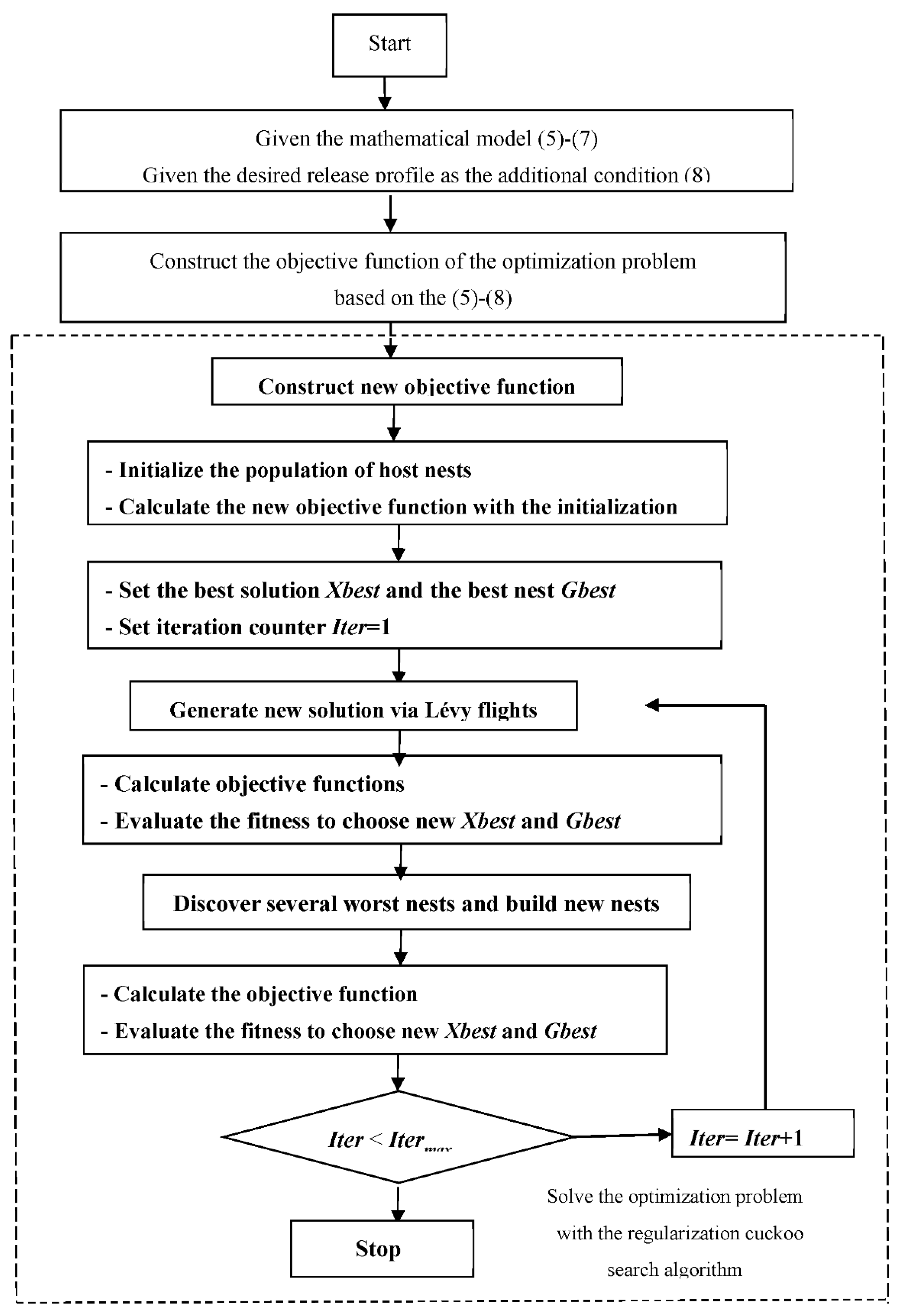
The objective function is chosen as $F=\parallel A\left(v\left(x\right)\right)-j(t,1){\parallel }_2^2+\alpha \parallel v\left(x\right){\parallel }_2^2,$ and the diffusion coefficient in the diffusion equation is $D(x)=x$. Since the different model layer means different drug initial concentration distributions, and different drug initial concentration distributions affect the drug release profile remarkably, the regularization cuckoo search algorithm is used to inverse the initial drug concentration distribution of the controlled release system containing different layers.

Case 1. Constant release rate, i.e., $j(t,1)=1, 0\le t\le 0.5$.

The statistical analysis of the error between the computational results and the desired release profile for the drug-controlled release system with different layers is shown in

Table 1. Statistical analysis of the error for optimization of the initial drug concentration (Case 1).

Number of Model Layers (NL)	Minimum Error	Maximum Error	Average Error	Standard Deviation (STD)
10	4.6868 × 10−2	5.2840 × 10−2	4.9685 × 10−2	2.2731 × 10−3
9	4.6877 × 10−2	5.2921 × 10−2	4.9782 × 10−2	2.2700 × 10−3
8	4.7442 × 10−2	5.3294 × 10−2	5.0374 × 10−2	2.1873 × 10−3
7	4.8341 × 10−2	5.6383 × 10−2	5.2114 × 10−2	3.0494 × 10−3
6	4.9309 × 10−2	5.7675 × 10−2	5.3654 × 10−2	3.0424 × 10−3
5	5.1370 × 10−2	5.8238 × 10−2	5.4712 × 10−2	2.4912 × 10−3
4	6.6118 × 10−2	7.2368 × 10−2	6.9111 × 10−2	2.2676 × 10−3
3	8.5613 × 10−2	9.6726 × 10−2	9.1050 × 10−2	3.9440 × 10−3
2	8.8341 × 10−2	9.8625 × 10−2	9.3813 × 10−2	3.7459 × 10−3

.

As shown in Table 1, the model layers number has a remarkable influence on the drug release profile. When the number of model layers reaches a certain number (for example, five), the error tends to stabilize with a small decrement. Meanwhile, if the number of model layers is less than five, the error is relatively larger. In order to further demonstrate the effect of the number of model layers on the drug release profile, the computational drug release flux for three different layer numbers, NL = 2, 4, 8, are shown in Figure 4. As we can see in Figure 4, when the number of model layers is equal to two or four, the computational drug release profile seems to be stable in the middle and last stages. However, the initial drug release curve oscillates seriously. If the number of model layers increases to eight, the drug release profile is closer to the desired release profile, and the drug release curve is relatively more stable. As a result, we seem to conclude that the increment of the number of model layers can improve computational precision. We think that maybe this is because we can control the initial drug concentration in the model more finely as the number of model layers increases. However, the number of model layers is not the more the better. It is seen that from Table 1 when the number of model layers is greater than or equal to five, there exists little difference between the errors of different model layers.

Therefore, based on the principle that the drug release model is as simple as possible and easy to implement, for obtaining the constant release rate, we choose NL = 9, namely, the controlled release system contains nine different initial concentrations of drugs, which are shown in

Table 2. Initial drug concentration at each layer of the drug-controlled release system with NL = 9 (Case 1).

Layer	Initial Drug Concentration	Layer	Initial Drug Concentration
1	5.1889	6	0.8378
2	8.8675 × 10−8	7	0.2367
3	7.2938 × 10−5	8	0.1851
4	1.4546 × 10−6	9	0.0015
5	1.1741 × 10−5	---	---

.

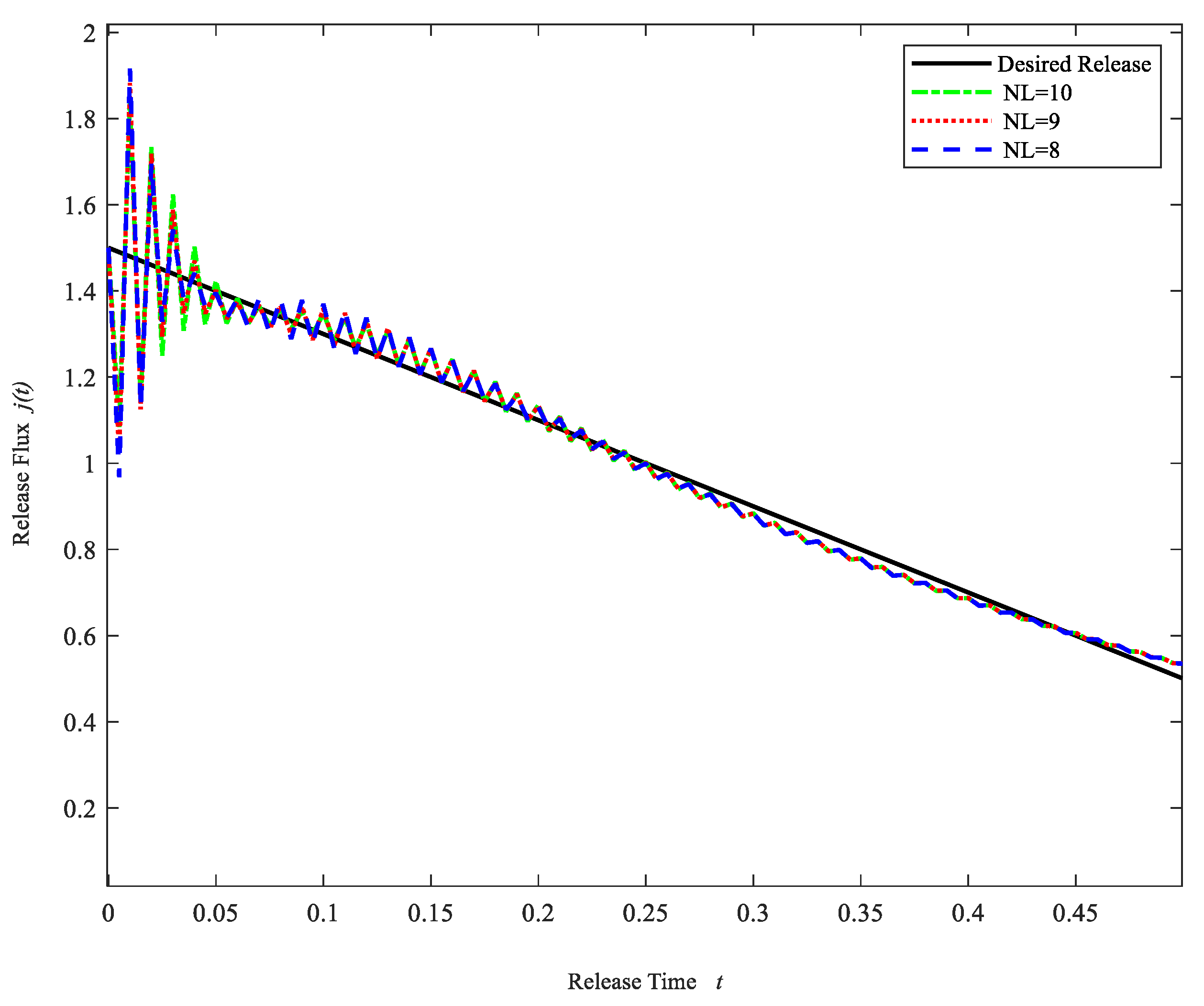
Case 2. Linearly decreasing release rate, i.e., $j(t)=1.5-2t, 0\le t\le 0.5$.

An approximately linearly increasing profile may be desired in some cases, e.g., to build up a tolerance for the chemical being delivered. In the previous case, we know that the desired release profile is not ideal when the number of model layers is less than five. Thus, in this case, only the numbers of model layers greater than five are considered.

Table 3. Statistical analysis of the error for optimization of the initial drug concentration (Case 2).

Number of Model Layers	Minimum Error	Maximum Error	Average Error	Standard Deviation (STD)
10	6.9173 × 10−3	7.5383 × 10−3	7.2307 × 10−3	2.2966 × 10−4
9	6.9279 × 10−3	7.5235 × 10−3	7.2310 × 10−3	2.2516 × 10−4
8	7.4410 × 10−3	8.0454 × 10−3	7.7378 × 10−3	2.2387 × 10−4
7	8.6647 × 10−3	9.1385 × 10−3	8.9192 × 10−3	1.8004 × 10−4
6	1.0437 × 10−2	1.6389 × 10−2	1.3515 × 10−2	2.1783 × 10−3

gives the statistical analysis of the error between the computational release profiles and the desired release profile for different layers. Figure 5 gives the computational drug release flux for three different layer numbers (NL = 8, 9, 10). As was expected, the computational release profiles are in good agreement with the desired release profile. It is also seen from Figure 5 and Table 3 that the error does not decrease significantly as the number of layers increases to a certain level. Therefore, we chose the number of layers NL = 9, i.e., the controlled release system contains nine layers. The drug initial concentrations of each layer are shown in

Table 4. Initial drug concentration at each layer of the drug-controlled release system with NL = 9 (Case 2).

Layer	Initial Drug Concentration	Layer	Initial Drug Concentration
1	3.3311	6	0.2843
2	0.0113	7	0.5049
3	4.671 × 10−3	8	0.2688
4	0.7379	9	0.0023
5	1.2939	---	---

.

Case 3. Non-linear release rate, i.e., $j(t)=\{\begin{array}{ll}24t& 0\le t\le 0.05\hfill \\ 1.2& 0.05<t\le 0.5\hfill \end{array}$.

Some situations demand a nonlinearly release rate, e.g., linearly increasing followed by a constant release, and without burst. A typical example is the delivery of some anticancer drugs. Similar to the previous two cases,

Table 5. Statistical analysis of the error for optimization of the initial drug concentration (Case 3).

Number of Model Layers (NL)	Minimum Error	Maximum Error	Average Error	Standard Deviation (STD)
10	6.3931× 10−2	6.9385 × 10−2	6.6460 × 10−2	2.0571 × 10−3
9	6.3957 × 10−2	6.9250 × 10−2	6.6455 × 10−2	2.0115 × 10−3
8	6.3907 × 10−2	6.8380 × 10−2	6.6139 × 10−2	1.7322 × 10−3
7	6.44304 × 10−2	7.0354 × 10−2	6.7909 × 10−2	2.3032 × 10−3
6	6.45556 × 10−2	7.1835 × 10−2	6.8771 × 10−2	2.7515 × 10−3

shows the statistical analysis of the error between the computational release profiles and the desired release profiles and Figure 6 gives the computational release profiles obtained by our algorithm. From the results of Table 5 and Figure 6, we can see that the error for NL = 8 is relatively smaller. Therefore, based on the comprehensive consideration of the computational cost and numerical accuracy, the drug-controlled release model can be chosen with NL = 8, namely, the drug-controlled release system contains eight layers. The initial concentrations of the drug at each layer are given in

Table 6. Initial drug concentration at each layer of the drug-controlled release system with NL = 8 (Case 3).

Layer	Initial Drug Concentration	Layer	Initial Drug Concentration
1	5.6699	5	1.100480
2	0	6	2.5771 ×10−13
3	2.9026 × 10−10	7	2.0444 × 10−2
4	7.0453 × 10−8	8	3.5613 × 10−14

.

Through the previous numerical results, we know that for the drug initial concentration optimization, all three desired release profiles are obtained to some extent by adjusting the initial drug concentration of the controlled release system. The best results are achieved when the desired release profile is linearly decreasing.

4.2. Optimization of Initial Drug Concentration and Diffusion Coefficient

As another example, in this section, we optimize both the initial drug concentration and the diffusion coefficient simultaneously and also consider the effect of different model layers on the drug release behavior. The objective function is set as

$$F\left(\begin{array}{c}\mathit{D}\left(x\right)\\ v\left(x\right)\end{array}\right)=\parallel A\left(\begin{array}{c}\mathit{D}\left(x\right)\\ v\left(x\right)\end{array}\right)-j(t,1){\parallel }_2^2+\alpha (\parallel \begin{array}{c}\mathit{D}\left(x\right)\\ v\left(x\right)\end{array}{\parallel }_2^2)$$

Case 1. Constant release rate.

Table 7. Statistical analysis of the error for optimization of the initial drug concentration and diffusion coefficient (Case 1).

Number of Model Layers	Minimum Error	Maximum Error	Average Error	Standard Deviation (STD)
10	2.2252 × 10−5	2.8253 × 10−5	2.4753 × 10−5	2.5987 × 10−6
9	1.4916 × 10−5	1.9454 × 10−5	1.7185 × 10−5	2.2691 × 10−6
8	4.2095 × 10−6	4.7346 × 10−6	4.4721 × 10−6	2.6252 × 10−7
7	8.3357 × 10−6	8.8566 × 10−6	8.5962 × 10−6	2.6043 × 10−7
6	4.1713 × 10−5	4.8743 × 10−5	4.5228 × 10−5	3.5153 × 10−6
5	4.6155 × 10−4	5.2155 × 10−4	4.8404 × 10−4	2.2776 × 10−5

shows the statistical analysis of the error between the computational release profiles and the desired release profile, and Figure 7 gives the computational release profiles obtained by using the regularization cuckoo search algorithm for three different model layers. As shown in Figure 7 and Table 7, when the number of model layers is greater than five, the errors are all close to 0 and the computational release profiles are very close to the desired release profiles. However, the error does not decrease significantly as the number of model layers increases, and the error reaches the minimum for NL = 8. Therefore, the drug-controlled release model with NL = 8 is taken as the suitable model.

Table 8. The initial drug concentration and diffusion coefficient at each layer of the drug-controlled release model for NL = 8 (Case 1).

Layer	Initial Drug Concentration	Diffusion Coefficient	Layer	Initial Drug Concentration	Diffusion Coefficient
1	2.971594	5.680510	5	4.040397	4.532567
2	4.164277	1.788725	6	0.736702	1.311099
3	3.652189	1.549742	7	2.165384	2.337045
4	0.677934	0.012543	8	0.010021	0.000014

shows the initial drug concentration and diffusion coefficient at each layer of the suitable model.

Case 2. Linearly decreasing release rate.

The statistical analysis of the error between the computational release profiles and the desired release profile is shown in

Table 9. Statistical analysis of the error for optimization of the initial drug concentration and diffusion coefficient (Case 2).

Number of Model Layers	Minimum Error	Maximum Error	Average Error	Standard Deviation (STD)
10	7.08120 × 10−3	8.23474 × 10−3	7.66596 × 10−3	4.77112 × 10−4
9	7.08071 × 10−3	8.23348 × 10−3	7.66470 × 10−3	4.44708 × 10−4
8	7.08067 × 10−3	8.12348 × 10−3	7.56798 × 10−3	4.24802 × 10−4
7	7.08063 × 10−3	8.07384 × 10−3	7.49849 × 10−3	3.90109 × 10−4
6	1.15463 × 10−2	2.01349 × 10−2	1.17253 × 10−2	6.59277 × 10−3

, and Figure 8 shows the computational release profiles obtained by using the regularization cuckoo search algorithm for three different model layers. From Table 9 and Figure 8, we can see that the drug release rate is more stable and at the same time the error decreases as the number of model layers increases. However, similar to the previous example, the error has no significant decrement when the number of model layers exceeds seven. Thus, the model of NL = 7 is taken as the appropriate model, and

Table 10. The initial drug concentration and diffusion coefficient at each layer of the controlled drug release model for NL = 7 (Case 2).

Layer	Initial Drug Concentration	Diffusion Coefficient	Layer	Initial Drug Concentration	Diffusion Coefficient
1	0.070579	0.001020	5	0.387654	28.693163
2	0.845192	80.939968	6	3.224124	19.295411
3	8.925855	3.103244	7	0.016351	0.000321
4	88.408474	1.687535	--	---	----

shows the initial drug concentration and drug diffusion coefficient at each layer of the appropriate model.

Case 3. Non-linear release rate.

As was expected, from

Table 11. Statistical analysis of the error for optimization of the initial drug concentration and diffusion coefficient (Case 3).

Number of Model Layers	Minimum Error	Maximum Error	Average Error	Standard Deviation (STD)
10	2.8713 × 10−3	3.5749 × 10−3	3.2271 × 10−3	2.8874 × 10−4
9	2.3261 × 10−3	3.048 × 10−3	2.7474 × 10−3	2.9134 × 10−4
8	2.2318 × 10−3	2.8479 × 10−3	2.5614 × 10−3	2.3003 × 10−4
7	2.9431 × 10−3	3.6841 × 10−3	3.3321 × 10−3	2.7650 × 10−4
6	3.8505 × 10−3	4.5278 × 10−3	4.1857 × 10−3	2.4239 × 10−4

, it is seen that the error gradually decreases as the number of model layers increases. However, when the number of model layers is greater than eight, the computational errors seem to become larger. The computational release profiles obtained by using the regularization cuckoo search algorithm for three different model layers in Figure 9 demonstrate that at the initial stage the computational release profiles are in good agreement with the desired release profile. As time goes on, the apparent fluctuation appears. The fluctuation is relatively flat. From the results of Table 11 and Figure 9, we choose the model with NL = 8 as the expected model.

Table 12. Initial drug concentration and diffusion coefficient at each layer of the drug-controlled release model for NL = 8 (Case 3).

Layer	Initial Drug Concentration	Diffusion Coefficient	Layer	Initial Drug Concentration	Diffusion Coefficient
1	2.884606	4.197390	5	5.982602	9.884345
2	9.887772	0.001	6	1.158236	0.739279
3	0	1.287389	7	3.417384	1.237826
4	3.596692	4.151442	8	0.011347	0.263782

shows the initial drug concentration and drug diffusion coefficient at each layer of the expected model.

5. Conclusions

In this paper, the optimization problem of drug release based on the multi-laminated drug-controlled release device was solved based on an inverse problem solution scheme.

Firstly, the optimization problem of drug release was transformed into the diffusion equation initial value inverse problem. Secondly, to solve this inverse problem, a new regularization cuckoo search algorithm has been proposed by combining the cuckoo search algorithm with the regularization technique. The adoption of the cuckoo search algorithm deduces the requirements of the objective function remarkably, and the use of the Tikhonov technique efficiently tackles the ill-posedness of the inverse problem. Finally, for three various desired release fluxes, the regularization cuckoo search algorithm was used to optimize the initial drug concentration and diffusion coefficient simultaneously. The numerical experiments show the capability of the proposed method to easily deal with the optimization problem of the drug-controlled release. The regularization cuckoo search algorithm has been successful at inverting the initial drug concentration and diffusion coefficient simultaneously.

Also shown in this paper is that the number of model layers has a large influence on the drug release rate. As seen in the examples, based on the comprehensive consideration of the computational cost and numerical accuracy, the optimal number of layers for the drug-controlled release model is given by comparing the computational results for different numbers of model layers. Another fact worth noting is the obvious advantage of the two-parameter optimization. The orders of average error obtained by the two-parameter optimization can reach ${10}^{-6}$ for the best case, whereas those of one-parameter optimization only reach ${10}^{-3}$. The simultaneous optimization of drug initial concentration and diffusion coefficient effectively reduce the error between the computational release rate and the desired release rate, which is of great benefit to achieve the desired drug release profiles.

In all, the satisfactory results obtained in this paper mean that the new regularization cuckoo search algorithm based on the inverse problem solution scheme exhibits its effectiveness and superiority, for the optimization problem of drug release based on the multi-laminated drug-controlled release device, to some extent. The proposed method is to be expected to solve more complicated cases, and this is an important direction for us to face in future.