Quadrature Rules for the F^m-Transform Polynomial Components

Abstract

The purpose of this paper is to reduce the complexity of computing the components of the integral $F^m$-transform, $m\ge 0$, whose analytic expressions include definite integrals. We propose to use nontrivial quadrature rules with nonuniformly distributed integration points instead of the widely used Newton–Cotes formulas. As the weight function that determines orthogonality, we choose the generating function of the fuzzy partition associated with the $F^m$-transform. Taking into account this fact and the fact of exact integration of orthogonal polynomials, we obtain exact analytic expressions for the denominators of the components of the $F^m$-transformation and their approximate analytic expressions, which include only elementary arithmetic operations. This allows us to effectively estimate the components of the $F^m$-transformation for $0\le m\le 3$. As a side result, we obtain a new method of numerical integration, which can be recommended not only for continuous functions, but also for strongly oscillating functions. The advantage of the proposed calculation method is shown by examples.

1. Introduction

The use of numerical integration methods manifests itself in various aspects of computation related to many problems of functional analysis, numerical solutions of differential and integral equations and their applications. In particular, the Gaussian quadrature rules considered in the monographs [1,2] are used in the analysis of the influence of numerical integration methods on the accuracy of solutions to various equations. As some examples, let us refer to fractional differential equations with a nonsingular Mittag–Leffler kernel [3], second-kind fuzzy Fredholm integral equations [4], variational equations [5,6] and second-order elliptic equations solved using non-parametric nonconforming quadrilateral elements [7].

In all the publications mentioned above, the Gaussian quadrature rules demonstrate their usefulness over other numerical integration methods in providing better approximation quality. In [8], this conclusion was confirmed for the finite element method based on the analysis of the dependence of the approximation quality on the numerical integration methods used. Similar dependencies were also studied in [9] for the p-version of finite elements and in [10] in connection with the approximation of eigenvalues. Later in [10,11], the above dependencies were discussed in the problem of approximation of linear functionals and approximation of eigenvalues.

As in the approaches mentioned above, the main attention in the proposed study is paid to the analysis of the effects of numerical integration in the calculation of the components of the fuzzy (F-)transforms of higher degrees. The importance of this seemingly narrow problem stems from the fact that the theory of F-transforms is regarded as a methodology for fuzzy functional analysis. The latter has become important with numerous applications in integral and differential calculus, image processing and computer vision, time series analysis, and neural network computing, see [12] and the references therein.

An extended view of this study shows its importance for any calculation of weighted projections of functional objects (images, signals, etc.) on an appropriate orthogonal basis, which may consist of eigenfunctions of various integral operators. This increases the value of the proposed results for the rapidly growing set of data-driven methodologies used in modern data analysis, now enriched with the F-transform, and especially its more powerful higher degree version [13].

Since the F-transform method requires the calculation of weighted orthogonal projections (F-transform components) onto orthogonal polynomials, it is important to reduce its complexity. Therefore, the main technical focus of this study is devoted to efficient and easy-to-implement methods of numerical integration. In addition, we will focus on three-point and four-point quadrature rules because it is generally not true that a quadrature formula with a large number of integration points guarantees optimal convergence [1,7].

To calculate the components of the $F^m$-transform of a higher degree, $m\ge 0$, the two-point Gaussian quadrature rules were first used in [14]. There we proposed an approximate analytical expression for the $F^1$-transform components.

In the current paper, we extend the applicability of these rules to $F^m$-transforms, where $m\le 3$. For general weight functions and their special triangular-shaped forms, exact analytic expressions are found for the integration points $x_1,\dots ,x_N$ and the weights $w_1,\dots ,w_N$, where $N\le 4$. This allows us to explicitly write the N-point quadrature Gauss formulas for $N\le 4$ and obtain exact expressions for the integrals of polynomial integrands up to degree 7. In combination with the inverse F-transform, this result significantly reduces the computational complexity of various approximations based on analytic expressions for the inverse F-transform. The $N\le 4$ constraint, offset by the corresponding number of fuzzy partition elements, guarantees that the inverse F-transform easily controls the quality of the approximation.

As an advantage of this approach, we show that low degree polynomials combined with a dense fuzzy partition provide comparable quality and lower computational complexity compared to high degree polynomial approximations over the entire domain. Another advantage is that the quadrature rule in its analytic form with local polynomial approximation based on the F-transform can be used as a technical step in an operational method [4] for solving (fuzzy) integral and differential equations.

Summing up, we can say that this article contributes and innovates two areas: approximation theory based on higher degree F-transforms and numerical methods of integration. In the second mentioned area, we give direct descriptions of integration points and weights for N-point Gaussian quadrature formulas, $N\le 4$, with an arbitrary positive weight function, and obtain exact expressions for integrals of (weighted) polynomials as integrands up to the degree 7. In the first direction, direct analytic expressions are proposed for the inverse $F^m$-transforms with $m\le 3$, where the latter include only arithmetic operations. This significantly reduces the computational complexity of this method (based on the integral F-transform) by eliminating the need for numerical integration.

The paper has the following structure: In Section 2, we give preliminaries related to the Gaussian quadrature formulas and the higher degree $F^m$-transforms. In Section 3, we formulate and give the technical details of our main result on 3- and 4-point Gaussian quadrature rules, where the weight function is the membership function of a fuzzy partition element. In Section 4, we define the 3- and 4-point Gauss quadrature rules for the particular weight function with a triangular shape.

Finally, in Section 6, on various numerical tests, we show the usefulness of the Gauss quadrature rules proposed here for calculating the components of the (direct and inverse) $F^m$-transform ($m\le 3$) and numerical integration.

2. Preliminaries

Below, we give a brief overview of the development of quadrature rules for numerical integration. Scientific research in this area is still in demand due to the many new forms of differential and integral calculus, including fuzzy and various fractional versions, see [3,4,5,6,7,9,11] and citations therein. Without going into numerous details, we recall the main facts related to the Gaussian quadrature rules [15,16,17,18,19] and show the most stable trends in their use.

The N-point Gaussian quadrature rule of the form (1) is a numerical integration rule that gives an exact result for polynomials of degree $2N-1$ or less with an appropriate choice of integration points $x_i$ and weights $w_i$, where $i=1,\dots ,N$, see e.g., [1,19]. Generalized formulation

$${\int }_a^b\omega \left(x\right)f\left(x\right)dx\approx \sum _{i=1}^N{w}_{i}f\left(x_i\right),$$

(1)

where $\omega :[a,b]\to {\mathbb{R}}_{+}$ is a weight function, was developed by Carl Gustav Jacobi in 1826. The choice of $\omega$ affects the choice of integration points $x_i$ and weights $w_i$, so if $p_1,\dots ,p_N$ are $\omega$-weighted orthogonal polynomials with degrees corresponding to their indices, then $x_1,\dots ,x_N$ are the roots of $p_N$. The weights $w_1,\dots ,w_N$ are found using the property that (1) is exact for polynomials of degree $2N-1$ or less. Moreover, if the weight function $\omega$ is symmetric with respect to the central point $(a+b)/2$, then the roots are symmetric with respect to this point, and the weights satisfy the condition: $w_i=w_{N+1-i}$. These two properties halve the computational complexity.

Depending on the choice of the weight function $\omega$, Gaussian quadrature rules are given by the names of their authors, see [15,18]. The most famous are Gauss–Legendre ($\omega \left(x\right)=1$), Gauss–Jacobi ($\omega \left(x\right)={(1-x)}^{\alpha }{(1+x)}^{\beta }$, $\alpha ,\beta >-1$) and Chebyshev–Gauss quadrature rules ($\omega \left(x\right)=1/\sqrt{1-x^2}$) considered on the interval $[-1,1]$. There are many algorithms for computing integration points $x_i$ and weights $w_i$ of Gaussian quadrature rules. The most popular are the Golub–Welsh algorithm [19] requiring O($N^2$) operations, Newton’s method for solving $p_N\left(x\right)=0$, requiring O($N^2$) operations, and asymptotic formulas for large N, requiring O(n) operations.

In this study, we develop quadrature Gaussian rules where the weight functions are the membership functions $A_1,\dots ,A_n:[a,b]\to [0,1]$ of an h-uniform fuzzy partition, and the corresponding orthogonal polynomials are defined as in [14]. The original idea was proposed in [14]. In this article, the 2-point Gaussian quadrature formula was found and applied to calculate the components of the $F^1$-transform. Based on the approach proposed in [14], we develop 3- and 4-point Gaussian quadrature formulas and use them to calculate the components of $F^m$-transformations, where $m\le 3$.

2.1. Fuzzy Partition

The notion of fuzzy partition has been evolved in the theory of fuzzy sets being adjusted to various requests to a space structure. The closest form to that which we use in this paper has been introduced in [20].

Definition 1

(Fuzzy partition). Let $[a,b]$ be an interval on $\mathbb{R}$, $n\ge 2$, and let $x_0$, $x_1$, …, $x_n$, $x_{n+1}$ be nodes such that $a=x_0=x_1<\dots <x_n=x_{n+1}=b$. We say that fuzzy sets $A_1,\dots ,A_n:[a,b]\to [0,1]$, which are identified with their membership functions, constitute a fuzzy partition of $[a,b]$ if for $k=1,\dots ,n$, they fulfill the following conditions:

• Normality: $A_k\left(x_k\right)=1$;
• Locality: $A_k\left(x\right)=0$ if $x\notin [x_{k-1},x_{k+1}]$;
• Continuity: $A_k\left(x\right)$ is continuous on $[a,b]$;
• Positiveness on support: $A_k\left(x\right)>0$ if $x\in (x_{k-1},x_{k+1})$;
• Ruspini condition: ${\displaystyle \sum _{k=1}^n}{A}_k\left(x\right)=1$, $x\in [a,b]$.

The membership functions $A_1,\dots ,A_n$ are called basic functions.

We say that the fuzzy partition $A_1,\dots ,A_n$, $n\ge 3$, is h-uniform, where $h=\frac{b-a}{n-1}$, if nodes $x_1,\dots ,x_n$ are h-equidistant, i.e., $x_{k+1}=x_k+h$, $k=1,\dots ,n-1$, and there exists an even function $A_0:[-1,1]\to [0,1]$ such that $A_0\left(0\right)=1$, and for all $k=1,\dots ,n$,

$$\begin{array}{c}\hfill A_k\left(x\right)=A_0\left(\frac{x-x_k}{h}\right),x\in [x_{k-1},x_{k+1}].\end{array}$$

(2)

We call $A_0$ a generating function of the uniform fuzzy partition.

Below, we introduce a set of Hilbert spaces, each of which is defined by a set of square-integrable functions on the corresponding element of the fuzzy partition and the basic function associated with it. We use the notation [14].

Let us fix $[a,b]$ and its fuzzy partition $A_1,\dots ,A_n,n\ge 3$. Let k be a fixed integer from $\{2,\dots ,n-1\}$, $A_k$ a basic function and $L_2\left(A_k\right)$ a set of square-integrable functions $f:[x_{k-1},x_{k+1}]\to \mathbb{R}$. Denote $L_2(a,b)$ as a set of functions $f:[a,b]\to \mathbb{R}$, such that

$${\int }_a^b{\left(f\left(x\right)\right)}^{2}dx<\infty .$$

Let us recall [14], and denote the inner product of f and g in $L_2\left(A_k\right)$ as

$${⟨f,g⟩}_k=\frac{{\int }_{x_{k-1}}^{x_{k+1}}f\left(x\right)g\left(x\right)A_k\left(x\right)dx}{{\int }_{x_{k-1}}^{x_{k+1}}{A}_k\left(x\right)dx}=\frac{{\int }_{x_{k-1}}^{x_{k+1}}f\left(x\right)g\left(x\right)A_k\left(x\right)dx}{h},$$

(3)

and the corresponding norm ${\parallel .\parallel }_k$ as

$${\parallel f\parallel }_k=\sqrt{{⟨f,f⟩}_k}.$$

We remind that the functions f and g $\in L_2\left(A_k\right)$ are orthogonal in $L_2\left(A_k\right)$ if ${⟨f,g⟩}_k=0$.

By [14], $L_2\left(A_k\right)$ together with the inner product (3) is a Hilbert space. Let k be a fixed integer from $\{2,...,n-1\}$, and let $\{1,x-x_k,{(x-x_k)}^2,\dots ,{(x-x_k)}^m\}$, $m\ge 0$, be a linearly independent system of polynomials, restricted to the support of $A_k$ and translated to the new origin $x_k$. Let us apply the Gram–Schmidt orthogonalization to the system $\{1,x-x_k,{(x-x_k)}^2,\dots ,{(x-x_k)}^m\}$ and convert it to the orthogonal polynomials $P_k^0,P_k^1,\dots ,P_k^m$ such that, for $l=0,\dots ,m-1$,

$$\begin{array}{c}\hfill P_k^0=1,P_k^{l+1}={(x-x_k)}^{l+1}-\sum _{i=0}^l{\lambda }_i^l{P}_k^i,\end{array}$$

(4)

where ${\lambda }_i^l=\frac{{⟨{(x-x_k)}^{l+1},P_k^i⟩}_k}{<P_k^i,P_k^i{>}_k}$, and ${⟨P_k^i,P_k^i⟩}_k\ne 0$, $i=0,\dots ,m$.

Remark 1.

It is easy to see that for all $k=2,...,n-1$; $r\in \mathbb{N}$ and $x\in [x_{k-1},x_{k+1}]$,

$$\begin{array}{cc}\hfill P_k^{2r}(-(x-x_k))& =P_k^{2r}(x-x_k),\hfill \\ \hfill P_k^{2r+1}(-(x-x_k))& =-P_k^{2r+1}(x-x_k).\hfill \end{array}$$

(5)

Example 1.

Let us give an example of the first five orthogonal polynomials $P_0^0,P_0^1,\dots ,P_0^4$ in $L_2\left(A_0\right)$, where $A_0:[-1,1]\to [0,1]$ is some fixed generating function and ${⟨·,·⟩}_0$ is the corresponding inner product:

$$\begin{array}{cc}\hfill P^0\left(x\right)=& 1,\hfill \\ \hfill P^1\left(x\right)=& x,\hfill \\ \hfill P^2\left(x\right)=& x^2-{⟨x^2,1⟩}_0=x^2-I_2^0,\hfill \\ \hfill P^3\left(x\right)=& x^3-\frac{{⟨x^4,1⟩}_0}{{⟨x^2,1⟩}_0}x=x^3-\frac{I_4^0}{I_2^0}x,\hfill \\ \hfill P^4\left(x\right)=& x^4-\frac{{⟨x^6,1⟩}_0-{⟨x^4,1⟩}_0{⟨x^2,1⟩}_0}{{⟨x^4,1⟩}_0-{⟨x^2,1⟩}_0^2}(x^2-{⟨x^2,1⟩}_0)-{⟨x^4,1⟩}_0=\hfill \\ \hfill & x^4-\frac{I_6^0-I_2^0{I}_4^0}{I_4^0-{\left(I_2^0\right)}^2}{x}^2+\frac{I_2^0{I}_6^0-{\left(I_2^0\right)}^2{I}_4^0}{I_4^0-{\left(I_2^0\right)}^2}-I_4^0=\hfill \\ \hfill & x^4-\frac{I_6^0-I_2^0{I}_4^0}{I_4^0-{\left(I_2^0\right)}^2}{x}^2+\frac{I_2^0{I}_6^0-{\left(I_4^0\right)}^2}{I_4^0-{\left(I_2^0\right)}^2}.\hfill \end{array}$$

Above, we have made use of the following notation:

$$I_2^0={\int }_{-1}^1{x}^2{A}_0\left(x\right)dx,I_4^0={\int }_{-1}^1{x}^4{A}_0\left(x\right)dx,I_6^0={\int }_{-1}^1{x}^6{A}_0\left(x\right)dx.$$

(6)

2.2. $F^m$-Transform

In this section, we repeat definitions of the direct and inverse $F^m$-transform as they appeared in [14]. Let k be a fixed integer from $\{2,...,n-1\}$ and $L_2^m\left(A_k\right)$ be a linear subspace of $L_2\left(A_k\right)$ spanned by $P_k^0,P_k^1,...,P_k^m$. It is easy to see that $L_2^m\left(A_k\right)$ consists of all polynomials of degree $l\le m$ restricted to the support of $A_k$. Moreover,

$$L_2^0\left(A_k\right)\subset L_2^1\left(A_k\right)\subset \dots L_2^m\left(A_k\right)\subset \dots .$$

Definition 2.

Let $f:[a,b]\to \mathbb{R}$ be a function from $L_2(a,b)$, and let $m\ge 0$ be a fixed integer. Denote $F_k^m$ as the k-th orthogonal projection of ${f|}_{[x_{k-1} , x_{k+1} ]}$ on $L_2^m\left(A_k\right)$, $k=2,\dots ,n-1$. We say that the $n-2$-tuple $(F_2^m,\dots ,F_{n-1}^m)$ is an $F^m$-transform of f with respect to $A_2,\dots ,A_{n-1}$, or formally,

$$\begin{array}{c}\hfill F^m\left[f\right]=(F_2^m,\dots ,F_{n-1}^m).\end{array}$$

(7)

$F_k^m$ is called the k-th $F^m$-transform component of f.

In [14], it was proved that

$$F_k^m=c_{k,0}{P}_k^0+c_{k,1}{P}_k^1+\dots +c_{k,m}{P}_k^m,$$

where

$$\begin{array}{cc}\hfill c_{k,i}& =\frac{{⟨f,P_k^i⟩}_k}{{⟨P_k^i,P_k^i⟩}_k}=\frac{{\int }_{x_{k-1}}^{x_{k+1}}f\left(x\right)P_k^i\left(x\right)A_k\left(x\right)dx}{{\int }_{x_{k-1}}^{x_{k+1}}{P}_k^i\left(x\right)P_k^i\left(x\right)A_k\left(x\right)dx},k=2,...,n-1,\hfill \end{array}$$

(8)

for $i=0,\dots ,m$.

An inverse $F^m$-transform of a function f is defined as a linear combination of basic functions with “coefficients” given by the $F^m$-transform components.

Definition 3.

Let $f:[a,b]\to \mathbb{R}$ be a given function, $m\ge 0$, and let $(F_2^m,\dots ,F_{n-1}^m)$ be the $F^m$-transform of f with respect to full fuzzy sets in the partition $A_2,\dots ,A_{n-1}$. Then, the following function $f_{F,n}^m:[a,b]\to \mathbb{R}$

$$f_{F,n}^m\left(x\right)=\sum _{k=2}^{n-1}{F}_k^m{A}_k\left(x\right)$$

(9)

is called the inverse $F^m$-transform of f with respect to $(F_2^m,\dots ,F_{n-1}^m)$ and $A_2,\dots ,A_{n-1}$.

In general, the inverse $F^m$-transform of $f\in L_2(a,b)$ is different from f. However for $m\ge 1$, it approximates f with the following quality estimate [14]:

$${\int }_{a+h}^{b-h}|f\left(x\right)-f_{F,n}^m\left(x\right)|dx\le O\left(h^2\right),$$

(10)

where the h-uniform partition $A_2,\dots ,A_{n-1}$ of $[a,b]$ fulfills the Ruspini condition on $[a+h,b-h]$, and functions f and $A_k$, $k=1,...,n$ are four times continuously differentiable on $[a,b]$.

2.3. The Quadrature Formula

To calculate the components of the $F^m$-transform of a higher degree, $m\ge 1$, it is necessary to compute a number of definite integrals given in (8). At least half of them are integrals of weighted polynomials, and other are integrals of functions with the same weight. For their precise and approximate computation, we propose to use Gaussian quadrature rules (1) specified by basic functions of the corresponding fuzzy partition. This idea was firstly used in [14] for the computation of the $F^1$-transform components. In the current paper, we extend the applicability of these rules to $F^m$-transforms, where $m\le 3$.

Let us fix $[a,b]$ and its h-uniform fuzzy partition $A_1,\dots ,A_n,n\ge 3$. Let k be a fixed integer from $\{2,\dots ,n-1\}$, $A_k$ a basic function, and $L_2\left(A_k\right)$ a set of square-integrable functions $f:[x_{k-1},x_{k+1}]\to \mathbb{R}$.

Definition 4

([14]). The N-point Gaussian quadrature rule of the form (1) with the weight function $A_k$ has the form

$$\begin{array}{c}\hfill {\int }_{x_{k-1}}^{x_{k+1}}f\left(x\right)A_k\left(x\right)dx\approx \sum _{i=1}^N{w}_{i}f\left(t_i^k\right).\end{array}$$

(11)

The integration points $t_i^k$ and weights $w_i$, $i=1,\dots ,N$, are assumed to be chosen so that (11) is exact for all polynomials of the highest possible degree.

Lemma 1

([14]). If $t_1^k,\dots ,t_N^k$ are roots of the polynomial $P_k^N$ and

$$\begin{array}{c}\hfill {\int }_{x_{k-1}}^{x_{k+1}}{P}_l\left(x\right)A_k\left(x\right)dx=\sum _{i=1}^N{w}_i{P}_l\left(t_i^k\right),\end{array}$$

(12)

holds true for all polynomials $P_l$ of degrees $0\le l\le N-1$ and some coefficients $w_1,...,w_N$, then (12) holds true for all polynomials $P_l$ of degree $0\le l\le 2N-1$.

Remark 2.

In the proposed contribution, we are looking for quadrature formulas that are exact for all polynomials of degrees 4 and 6, respectively. By lemma 1 we see that the values $N=3$ and $N=4$, respectively, are suitable for this purpose.

3. Main Results

In this section, we will discuss how to construct 3- and 4-Gaussian quadrature formulas with the membership function $A_k$ as a weight function. We will discuss 3- and 4-quadrature formulas in the two subsequent subsections separately. Then we will show how to use these results and obtain exact analytical expressions for the denominators of components $c_{k,2}$ and $c_{k,3}$ given in (8), where $k=2,3$. This becomes possible because their integrands are polynomials of the fourth and sixth degrees respectively so that the proposed 3- and 4- Gaussian quadrature rules are exact for these polynomials.

Assume that interval $[a,b]$ has an h-uniform fuzzy partition $A_1,...,A_n$ which will be fixed throughout this section. Since the domains of membership functions $A_1$ and $A_n$ are only half size of domains of other membership functions, we will consider two separate cases:

(i)

Regular, when $k=2,...,n-1$.

(ii)

Boundary, when $k=1,n$.

Let us fix the value of k, $1\le k\le n$, and make some useful notations

$$\begin{array}{c}\hfill I_2={\int }_{x_{k-1}}^{x_{k+1}}{(x-x_k)}^2{A}_k\left(x\right)dx,\\ \hfill I_4={\int }_{x_{k-1}}^{x_{k+1}}{(x-x_k)}^4{A}_k\left(x\right)dx,\\ \hfill I_6={\int }_{x_{k-1}}^{x_{k+1}}{(x-x_k)}^6{A}_k\left(x\right)dx,\end{array}$$

(13)

$$\begin{array}{c}\hfill \tilde{\delta }=\sqrt{\frac{I_2}{h}},\delta =\sqrt{\frac{I_4}{I_2}}.\end{array}$$

(14)

3.1. Domain Extension

In this subsection, we redefine the F-transform components for the boundary case (ii), i.e., for the case $k=1$ or $k=n$. At first, we extend the given interval $[a,b]$ to $[a-h,b+h]$, where h is a parameter of an h-uniform fuzzy partition.

Let us denote $L_2\left(A_1\right)$ and $L_2\left(A_n\right)$ as

$$\begin{array}{cc}\hfill L_2\left(A_1\right)& =\left\{f:[a-h,x_2]\to \mathbb{R}|{\int }_{a-h}^{x_2}{f}^2\left(x\right)dx<\infty \right\},\hfill \\ \hfill L_2\left(A_n\right)& =\left\{f:[x_{n-1},b+h]\to \mathbb{R}|{\int }_{x_{n-1}}^{b+h}{f}^2\left(x\right)dx<\infty \right\}.\hfill \end{array}$$

Extend domains of $A_1$ and $A_n$ to $[a-h,x_2]$ and $[x_{n-1},b+h]$, respectively, and define (as in [21])

$$\begin{array}{cc}\hfill A_1^{ex}\left(x\right)& =\left\{\begin{array}{cc}{A}_1\left(x\right)\hfill & \mathrm{for}\mathrm{all}x\in [a,x_2],\hfill \\ A_1(2a-x)\hfill & \mathrm{for}\mathrm{all}x\in [a-h,a),\hfill \end{array}\right.\hfill \end{array}$$

(15)

$$\begin{array}{cc}\hfill A_n^{ex}\left(x\right)& =\left\{\begin{array}{cc}{A}_n\left(x\right)\hfill & \mathrm{for}\mathrm{all}x\in [x_{n-1},b],\hfill \\ A_n(2b-x)\hfill & \mathrm{for}\mathrm{all}x\in (b,b+h].\hfill \end{array}\right.\hfill \end{array}$$

(16)

The corresponding inner products are defined in the same way as in (3):

$$\begin{array}{c}\hfill {⟨f,g⟩}_1=\frac{{\int }_{a-h}^{x_2}f\left(x\right)g\left(x\right)A_1^{ex}\left(x\right)dx}{h},\mathrm{for}\mathrm{all}f,g\in L_2\left(A_1\right),\\ \hfill {⟨f,g⟩}_n=\frac{{\int }_{x_{n-1}}^{b+h}f\left(x\right)g\left(x\right)A_n^{ex}\left(x\right)dx}{h},\mathrm{for}\mathrm{all}f,g\in L_2\left(A_n\right).\end{array}$$

(17)

Similarly to Example 1, we apply the Gram–Schmidt orthogonalization and construct the orthogonal polynomials $P_1^0,...,P_1^m$ and $P_n^0,...,P_n^m$ as follows:

$$\begin{array}{c}\hfill P_1^0\left(x\right)=1,P_1^{l+1}={(x-a)}^{l+1}-\sum _{i=0}^l{\lambda }_{i,1}^l{P}_0^i\left(x\right),\mathrm{for}\mathrm{all}x\in [a-h,x_2],\\ \hfill P_n^0\left(x\right)=1,P_n^{l+1}={(x-b)}^{l+1}-\sum _{i=0}^l{\lambda }_{i,n}^l{P}_0^i\left(x\right),\mathrm{for}\mathrm{all}x\in [x_{n-1},b+h],\end{array}$$

(18)

where ${\lambda }_{i,1}^l=\frac{<{(x-a)}^{l+1},P_1^i{>}_1}{<P_1^i,P_1^i{>}_1}$, ${\lambda }_{i,n}^l=\frac{<{(x-b)}^{l+1},P_n^i{>}_n}{<P_n^i,P_n^i{>}_n}$, and $<P_1^i,P_1^i{>}_1\ne 0$, $<P_n^i,P_n^i{>}_n\ne 0$, $i=0,\dots ,l$.

Let $L_2^m\left(A_1\right)$($L_2^m\left(A_n\right)$) be a linear subspace of $L_2\left(A_1\right)$($L_2\left(A_n\right)$) spanned by $P_1^0,...,P_1^m$($P_n^0,...,P_n^m$). It is easy to see that $L_2^m\left(A_1\right)$ and $L_2^m\left(A_n\right)$ have all properties of $L_2^m\left(A_k\right)$, $k=2,...,n-1$.

Let us extend $f\in L_2(a,b)$ to $f^{ex}$ (similar to [21]), where $f^{ex}:[a-h,b+h]\to \mathbb{R}$,

$$\begin{array}{cc}\hfill f^{ex}\left(x\right)& =\left\{\begin{array}{cc}f\left(x\right)\hfill & \mathrm{if}x\in [a,b],\hfill \\ f(2a-x)\hfill & \mathrm{if}x\in [a-h,a),\hfill \\ f(2b-x)\hfill & \mathrm{if}x\in (b,b+h].\hfill \end{array}\right.\hfill \end{array}$$

(19)

Obviously, $f^{ex}{|}_{[a-h,x_2]}\in L_2^m\left(A_1\right)$ and $f^{ex}{|}_{[x_{n-1},b+h]}\in L_2^m\left(A_n\right)$.

Definition 5.

Let $f:[a,b]\to \mathbb{R}$ be a function from $L_2(a,b)$ and $f^{ex}$ be its extension to $[a-h,b+h]$. Define the $F^m$-transform components $F_1^m$ and $F_n^m$$f^{ex}$ similarly to Definition 2 and as follows:

$$\begin{array}{cc}\hfill F_1^m& =c_{1,0}{P}_1^0+c_{1,1}{P}_1^1+...+c_{1,m}{P}_1^m,\hfill \\ \hfill F_n^m& =c_{n,0}{P}_n^0+c_{n,1}{P}_n^1+...+c_{n,m}{P}_n^m,\hfill \end{array}$$

where for $i=0,...,m$ (as in (8)),

$$\begin{array}{cc}\hfill c_{1,i}& =\frac{{⟨f^{ex},P_1^i⟩}_1}{{⟨P_1^i,P_1^i⟩}_1}=\frac{{\int }_{a-h}^b{f}^{ex}\left(x\right)P_1^i\left(x\right)A_1^{ex}\left(x\right)dx}{{\int }_{a-h}^b{P}_1^i\left(x\right)P_1^i\left(x\right)A_1^{ex}\left(x\right)dx}=\frac{2{\int }_a^{x_2}f\left(x\right)P_1^i\left(x\right)A_1\left(x\right)dx}{{\int }_{a-h}^{x_2}{P}_1^i\left(x\right)P_1^i\left(x\right)A_1^{ex}\left(x\right)dx},\hfill \\ \hfill c_{n,i}& =\frac{{⟨f^{ex},P_n^i⟩}_n}{{⟨P_n^i,P_n^i⟩}_n}=\frac{{\int }_a^{b+h}{f}^{ex}\left(x\right)P_n^i\left(x\right)A_n^{ex}\left(x\right)dx}{{\int }_a^{b+h}{P}_n^i\left(x\right)P_n^i\left(x\right)A_n^{ex}\left(x\right)dx}=\frac{2{\int }_{x_{n-1}}^{b}f\left(x\right)P_n^i\left(x\right)A_n\left(x\right)dx}{{\int }_{x_{n-1}}^{b+h}{P}_n^i\left(x\right)P_n^i\left(x\right)A_n^{ex}\left(x\right)dx}.\hfill \end{array}$$

(20)

The n-tuple $(F_1^m,F_2^m,...,F_{n-1}^m,F_n^m)$ is an extended $F^m$-transform of $f^{ex}$ with respect to the extended partition $A_1^{ex},A_2,\dots ,A_{n-1},A_n^{ex}$, or formally,

$$F^m\left[f^{ex}\right]=(F_1^m,...,F_n^m).$$

Accordingly, we extend the Definition 3 of the inverse $F^m$-transformat to the function $f^{ex}$. By the quality estimate (10), we have

$$\begin{array}{c}\hfill {\int }_a^b|f\left(x\right)-f_{ex}^{m,n}\left(x\right)|dx\le O\left(h^2\right),\end{array}$$

where the h-uniform partition $A_1^{ex},A_2,...A_{n-1},A_n^{ex}$ of $[a,b]$ fulfills the Ruspini condition on $[a,b]$.

3.2. 3-Point Quadrature Rule with Weight Function $A_k$

In this subsection, we find the parameters of the 3-point quadrature formula (11) specified in Definition 4. By Lemma 1, this means to find the roots $t_1^k,t_2^k,t_3^k$ of the polynomial $P_k^3\left(x\right)$ and the coefficients $w_1,w_2,w_3$, such that

$$\begin{array}{c}\hfill {\int }_{x_{k-1}}^{x_{k+1}}{P}_l\left(x\right)A_k\left(x\right)dx=w_1{P}_l\left(t_1^k\right)+w_2{P}_l\left(t_2^k\right)+w_3{P}_l\left(t_3^k\right),\end{array}$$

(21)

is satisfied for all polynomials $P_l$ of degree $0\le l\le 2$.

By Example 1,

$$\begin{array}{c}\hfill P_k^3\left(x\right)={(x-x_k)}^3-\frac{I_4}{I_2}(x-x_k),\end{array}$$

(22)

and it is orthogonal to $P_k^0,P_k^1,P_k^2$ with respect to (3). It is easy to see that the roofs of $P_k^3$ are

$$\begin{array}{c}\hfill \left\{\begin{array}{c}{t}_1^k=x_k-\sqrt{\frac{I_4}{I_2}}=x_k-\delta ,\hfill \\ t_2^k=x_k,\hfill \\ t_3^k=x_k+\sqrt{\frac{I_4}{I_2}}=x_k+\delta .\hfill \end{array}\right.\end{array}$$

(23)

Let us denote

$$\begin{array}{c}\hfill \rho =\frac{I_2^2}{2h{I}_4},w_1=w_3=h\rho ,w_2=h(1-2\rho ).\end{array}$$

(24)

First, consider the case when $k=2,...,n-1$.

Lemma 2.

For all polynomials $P_l$ of degree l, $0\le l\le 2$, the equality

$$\begin{array}{c}\hfill {\int }_{x_{k-1}}^{x_{k+1}}{P}_l\left(x\right)A_k\left(x\right)dx=w_1{P}_l\left(t_1^k\right)+w_2{P}_l\left(t_2^k\right)+w_3{P}_l\left(t_3^k\right),\end{array}$$

(25)

where $w_1,w_2,w_3$ are specified in (24), holds true.

Proof. 

Case 1: For $l=0$, we have $P_0\left(x\right)=\alpha$ with $\alpha \in \mathbb{R}$. Firstly, we compute the left side of (25):

$$\begin{array}{cc}\hfill {\int }_{x_{k-1}}^{x_{k+1}}{P}_0\left(x\right)A_k\left(x\right)dx& ={\int }_{x_{k-1}}^{x_{k+1}}\alpha A_k\left(x\right)dx=\alpha h=h(\rho \alpha +(1-2\rho )\alpha +\rho \alpha )\hfill \\ \hfill & =h(\rho P_0\left(t_1^k\right)+(1-2\rho )P_0\left(t_2^k\right)+\rho P_0\left(t_3^k\right))\hfill \\ \hfill & =w_1{P}_0\left(t_1^k\right)+w_2{P}_0\left(t_2^k\right)+w_3{P}_0\left(t_3^k\right).\hfill \end{array}$$

Case 2: For $l=1$, we have $P_1\left(x\right)=\alpha +\beta x$ with $\alpha ,\beta \in \mathbb{R}$. We compute the left side of (25)

$$\begin{array}{cc}\hfill {\int }_{x_{k-1}}^{x_{k+1}}{P}_1\left(x\right)A_k\left(x\right)dx& ={\int }_{x_{k-1}}^{x_{k+1}}(\alpha +\beta x_k)A_k\left(x\right)+\beta {\int }_{x_{k-1}}^{x_{k+1}}(x-x_k)A_k\left(x\right)dx\hfill \\ \hfill & =(\alpha +\beta x_k){\int }_{x_{k-1}}^{x_{k+1}}{A}_k\left(x\right)dx=h(\alpha +\beta x_k).\hfill \end{array}$$

(26)

On the right hand side of (25), we have

$$\begin{array}{cc}\hfill P_1\left(t_1^k\right)& =P_1(x_k-\delta )=\alpha +\beta (x_k-\delta )=\alpha +\beta x_k-\beta \delta ,\hfill \\ \hfill P_1\left(t_2^k\right)& =P_1\left(x_k\right)=\alpha +\beta x_k,\hfill \\ \hfill P_1\left(t_3^k\right)& =P_1(x_k+\delta )=\alpha +\beta (x_k+\delta )=\alpha +\beta x_k+\beta \delta .\hfill \end{array}$$

By the direct computation, we see that the left hand side of (25) is equal to its right hand side:

$$\begin{array}{cc}\hfill {\int }_{x_{k-1}}^{x_{k+1}}{P}_1\left(x\right)A_k\left(x\right)dx& =h(\alpha +\beta x_k)\hfill \\ \hfill & =h\left(\rho (\alpha +\beta x_k-\beta \delta )+(1-2\rho )(\alpha +\beta x_k)+\rho (\alpha +\beta x_k+\beta \delta )\right)\hfill \\ \hfill & =w_1{P}_1\left(t_1^k\right)+w_2{P}_1\left(t_2^k\right)+w_3{P}_1\left(t_3^k\right).\hfill \end{array}$$

Case 3: For $l=2$, we have $P_2\left(x\right)=\alpha +\beta x+\gamma x^2$ with $\alpha ,\beta ,\gamma \in \mathbb{R}$. At first, we rewrite $P_2\left(x\right)$ into

$$\begin{array}{cc}\hfill P_2\left(x\right)& =\alpha +\beta x+\gamma x^2=\gamma \left({(x-x_k)}^2-\frac{I_2}{h}\right)+(2\gamma x_k+\beta )(x-x_k)+\gamma x_k^2+\beta x_k+\alpha +\gamma \frac{I_2}{h}\hfill \\ \hfill & =\gamma P_k^2\left(x\right)+(2\gamma x_k+\beta )P_k^1\left(x\right)+\gamma x_k^2+\beta x_k+\alpha +\gamma \frac{I_2}{h}.\hfill \end{array}$$

Then, the left hand side of (25) becomes

$$\begin{array}{cc}\hfill {\int }_{x_{k-1}}^{x_{k+1}}{P}_2\left(x\right)A_k\left(x\right)dx=& \gamma {\int }_{x_{k-1}}^{x_{k+1}}{P}_k^2\left(x\right)A_k\left(x\right)dx+(2\gamma x_k+\beta ){\int }_{x_{k-1}}^{x_{k+1}}{P}_k^1\left(x\right)A_k\left(x\right)dx\hfill \\ \hfill & +\left(\gamma x_k^2+\beta x_k+\alpha +\gamma \frac{I_2}{h}\right){\int }_{x_{k-1}}^{x_{k+1}}{A}_k\left(x\right)dx\hfill \\ \hfill =& h\left(\gamma x_k^2+\beta x_k+\alpha +\gamma \frac{I_2}{h}\right)=h\left(\alpha +\beta x_k+\gamma x_k^2+2\gamma \frac{I_2^2}{2h{I}_4}\frac{I_4}{I_2}\right)\hfill \\ \hfill =& h\left(\gamma x_k^2+\beta x_k+\alpha +2\rho \gamma {\delta }^2\right).\hfill \end{array}$$

(27)

Using

$$\begin{array}{cc}\hfill P_2\left(t_1^k\right)& =P_2(x_k-\delta )=\alpha +\beta (x_k-\delta )+\gamma {(x_k-\delta )}^2=\alpha +\beta x_k+\gamma x_k^2-\beta \delta -2\gamma x_k{\delta }^2+\gamma {\delta }^2,\hfill \\ \hfill P_2\left(t_2^k\right)& =P_2\left(x_k\right)=\alpha +\beta x_k+\gamma x_k^2,\hfill \\ \hfill P_2\left(t_3^k\right)& =P_2(x_k+\delta )=\alpha +\beta (x_k+\delta )+\gamma {(x_k+\delta )}^2=\alpha +\beta x_k+\gamma x_k^2+\beta \delta +2\gamma x_k{\delta }^2+\gamma {\delta }^2,\hfill \end{array}$$

we easily come to

$$\begin{array}{c}\hfill \rho P_2\left(t_1^k\right)+(1-2\rho )P_2\left(t_2^k\right)+\rho P_2\left(t_3^k\right)=\alpha +\beta x_k+\gamma x_k^2+2\rho \gamma {\delta }^2.\end{array}$$

(28)

By (27) and (28),

$$\begin{array}{cc}\hfill {\int }_{x_{k-1}}^{x_{k+1}}{P}_2\left(x\right)A_k\left(x\right)dx& =h\left(\rho P_2\left(t_1^k\right)+(1-2\rho )P_2\left(t_2^k\right)+\rho P_2\left(t_3^k\right)\right)\hfill \\ \hfill & =w_1{P}_2\left(t_1^k\right)+w_2{P}_2\left(t_2^k\right)+w_3{P}_2\left(t_3^k\right).\hfill \end{array}$$

Therefore, Equation (25) holds true for all polynomials $P_l$ of $0\le l\le 2.$ □

Corollary 1.

Let $[a,b]$ be an interval on $\mathbb{R}$, and $A_1,...,A_n$ be an h-uniform fuzzy partition of $[a,b]$, and $\alpha ,\beta ,\gamma$ be arbitrary real numbers. Then

$$\begin{array}{cc}\hfill {\int }_{x_{k-1}}^{x_{k+1}}(\alpha +\beta x)A_k\left(x\right)dx& =h(\alpha +\beta x_k),\hfill \\ \hfill {\int }_{x_{k-1}}^{x_{k+1}}(\alpha +\beta x+\gamma x^2)A_k\left(x\right)dx& =h\left(\gamma x_k^2+\beta x_k+\alpha +\gamma \frac{I_2}{h}\right).\hfill \end{array}$$

Proof. 

Based on Equations (26) and (27). □

Corollary 2.

The quadrature formula (25) holds true for all polynomials of degree $0\le l\le 5$.

Now we consider the cases $k=1$ and $k=n$ where the 3-point quadrature rule (11), specified by $N=3$, and parameters in (23) and (24), is used for a general $L_2(a,b)$ function including polynomials. Therefore, this rule gives an approxamate value of the corresponding integral.

Lemma 3.

Let $[a,b]$ be arbitrary interval and $A_1,...,A_n$ is its h-uniform fuzzy partition. Let $A_1^{ex},A_n^{ex}$ extend $A_1$ and $A_n$ as in (15) and (16), respectively. For any $f\in L_2(a,b)$ and its extension $f^{ex}\in L_2(a-h,b+h)$,

$$\begin{array}{cc}\hfill {\int }_a^{x_2}f\left(x\right)A_1\left(x\right)dx& \approx w_{3}f\left(t_3^1\right)+\frac{1}{2}{w}_{2}f\left(t_2^1\right),\hfill \end{array}$$

(29)

$$\begin{array}{cc}\hfill {\int }_{x_{n-1}}^{b}f\left(x\right)A_{n}dx& \approx w_{1}f\left(t_1^n\right)+\frac{1}{2}{w}_{2}f\left(t_2^n\right),\hfill \end{array}$$

(30)

where $w_1,w_2,w_3$ are in (24).

Proof. 

On the left hand side of (29), we have

$$\begin{array}{cc}\hfill {\int }_a^{x_2}f\left(x\right)A_1\left(x\right)dx& =\frac{1}{2}{\int }_{a-h}^{x_2}{f}^{ex}\left(x\right)A_1^{ex}\left(x\right)dx\hfill \\ \hfill & \approx \frac{h}{2}(\rho f^{ex}(a-\delta )+(1-2\rho )f^{ex}\left(a\right)+\rho f^{ex}(a+\delta ))\hfill \\ \hfill & =h\left(\rho f(a+\delta )+\frac{1}{2}(1-2\rho )f\left(a\right)\right)=w_{3}f\left(t_3^1\right)+\frac{1}{2}{w}_{2}f\left(t_2^1\right).\hfill \end{array}$$

Equation (30) can be proved similarly. □

Theorem 1.

Let $A_1,...,A_n$ be the h-uniform fuzzy partition of an interval $[a,b]$, $f\in L_2(a,b)$ and n-tuple $(F_1^2,...,F_n^2)$ is an the extended $F^2$-transform of $f^{ex}$ with respect to $A_1^{ex},...,A_n^{ex}$. Then for any $k=1,...,n$, the calculation of the component of the $F^2$-transform $F_k^2$, where

$$\begin{array}{c}\hfill F_k^2=c_{k,0}{P}_k^0+c_{k,1}{P}_k^1+c_{k,2}{P}_k^2,\end{array}$$

can be performed using approximate analytical expressions for the coefficients $c_{k,0},c_{k,1},c_{k,2}$, based on the three-point quadrature rules (11) given by $N=3$, and the parameters in (23) and (24). Specifically,

$$\begin{array}{cc}\hfill c_{k,0}& \approx \frac{{\sum }_{i=1}^3{w}_{i}f\left(t_i^k\right)}{h},\mathrm{for}\mathrm{all}k=2,...,n-1,\hfill \\ \hfill c_{1,0}& \approx \frac{2w_{3}f\left(t_3^1\right)+w_{2}f\left(t_2^1\right)}{h},\hfill \\ \hfill c_{n,0}& \approx \frac{2w_{1}f\left(t_1^n\right)+w_{2}f\left(t_2^n\right)}{h}\hfill \\ \hfill c_{k,1}& \approx \frac{{\sum }_{i=1}^3{w}_i(t_i^k-x_k)f\left(t_i^k\right)}{h{\tilde{\delta }}^2},\mathrm{for}\mathrm{all}k=2,...,n-1,\hfill \\ \hfill c_{1,1}& \approx \frac{2w_3\delta f\left(t_3^1\right)}{h{\tilde{\delta }}^2},\hfill \\ \hfill c_{n,1}& \approx \frac{-2w_1\delta f\left(t_1^n\right)}{h{\tilde{\delta }}^2},\hfill \\ \hfill c_{k,2}& \approx \frac{{\sum }_{i=1}^3{w}_i\left[{(t_i^k-x_k)}^2-{\tilde{\delta }}^2\right]f\left(t_i^k\right)}{h(2\rho {\delta }^4-{\tilde{\delta }}^4)},\mathrm{for}\mathrm{all}k=2,...,n-1,\hfill \\ \hfill c_{1,2}& \approx \frac{2w_3\left({\delta }^2-{\tilde{\delta }}^2\right)f\left(t_3^1\right)-w_2{\tilde{\delta }}^{2}f\left(t_2^1\right)}{h(2\rho {\delta }^4-{\tilde{\delta }}^4)},\hfill \\ \hfill c_{n,2}& \approx \frac{2w_1\left({\delta }^2-{\tilde{\delta }}^2\right)f\left(t_1^n\right)-w_2{\tilde{\delta }}^{2}f\left(t_2^n\right)}{h(2\rho {\delta }^4-{\tilde{\delta }}^4)}.\hfill \end{array}$$

(31)

Proof. 

First of all, we note that an exact analytical estimate of the denominators in the expressions for $c_{k,0},c_{k,1}$ was proved in [14]. Therefore, we will focus on the calculation of $c_{k,2}$, the general expression of which is given in (8).

We begin with the estimation of $I_2$ and $I_4$. Using Lemma 2 and Theorem 4 in [14], we have

$$\begin{array}{cc}\hfill I_2& ={\int }_{x_{k-1}}^{x_{k+1}}{(x-x_k)}^2{A}_k\left(x\right)dx=\frac{h}{2}\left({(t_1^k-x_k)}^2+{(t_2^k-x_k)}^2\right)=\frac{h}{2}2{\tilde{\delta }}^2=h{\tilde{\delta }}^2,\hfill \\ \hfill I_4& ={\int }_{a-h}^{x_2}{(x-a)}^4{A}_1^{ex}\left(x\right)dx={\int }_{x_{n-1}}^{b+h}{(x-b)}^4{A}_n^{ex}\left(x\right)dx={\int }_{x_{k-1}}^{x_{k+1}}{(x-x_k)}^4{A}_k\left(x\right)dx\hfill \\ & =h\left(\rho {(x_k-\delta -x_k)}^4+(1-2\rho ){(x_k-x_k)}^4+\rho {(x_k+\delta -x_k)}^4\right)=2h\rho {\delta }^4.\hfill \end{array}$$

Therefore, for $k=2,...,n-1$, the denominator of $c_{k,2}$ is

$$\begin{array}{cc}\hfill {\int }_{x_{k-1}}^{x_{k+1}}{\left(P_k^2\left(x\right)\right)}^2{A}_k\left(x\right)dx=& {\int }_{x_{k-1}}^{x_{k+1}}{\left[{(x-x_k)}^2-{\tilde{\delta }}^2\right]}^2{A}_k\left(x\right)dx\hfill \\ \hfill =& {\int }_{x_{k-1}}^{x_{k+1}}\left[{(x-x_k)}^4-2{\tilde{\delta }}^2{(x-x_k)}^2+{\tilde{\delta }}^4\right]A_k\left(x\right)dx\hfill \\ \hfill =& {\int }_{x_{k-1}}^{x_{k+1}}{(x-x_k)}^4{A}_k\left(x\right)dx-2{\tilde{\delta }}^2{\int }_{x_{k-1}}^{x_{k+1}}{(x-x_k)}^2{A}_k\left(x\right)dx\hfill \\ \hfill & +{\tilde{\delta }}^4{\int }_{x_{k-1}}^{x_{k+1}}{A}_k\left(x\right)dx\hfill \\ \hfill =& I_4-2{\tilde{\delta }}^2{I}_2+h{\tilde{\delta }}^4=2h\rho {\delta }^4-2h{\tilde{\delta }}^4+h{\tilde{\delta }}^4=h(2\rho {\delta }^4-{\tilde{\delta }}^4).\hfill \end{array}$$

Obviously, the denominators of $c_{1,2}$ and $c_{n,2}$

$$\begin{array}{cc}\hfill {\int }_{a-h}^{x_2}{\left(P_1^2\left(x\right)\right)}^2{A}_1^{ex}\left(x\right)dx& ={\int }_{x_{n-1}}^{b+h}{\left(P_n^2\left(x\right)\right)}^2{A}_n^{ex}\left(x\right)dx\hfill \\ \hfill & ={\int }_{x_{k-1}}^{x_{k+1}}{\left(P_k^2\left(x\right)\right)}^2{A}_k\left(x\right)dx=h(2\rho {\delta }^4-{\tilde{\delta }}^4).\hfill \end{array}$$

Apply the Formulas (29) and (30) to calculate the numerators of the components, the theorem is proved. □

3.3. 4-Point Quadrature Rule with Weight Function $A_k$

In this subsection, we construct the quadrature formula specified in Definition 4 where $N=4$. By Lemma 1, this means to find the roofs $t_1^k,t_2^k,t_3^k,t_4^k$ of $P_k^4\left(x\right)$ and coefficients $w_1,w_2,w_3,w_4$ that satisfy

$$\begin{array}{c}\hfill {\int }_{x_{k-1}}^{x_{k+1}}{P}_l\left(x\right)A_k\left(x\right)dx=w_1{P}_l\left(t_1^k\right)+w_2{P}_l\left(t_2^k\right)+w_3{P}_l\left(t_3^k\right)+w_4{P}_l\left(t_4^k\right),\end{array}$$

(32)

for all polynomials $P_l$ of degree $0\le l\le 3$.

Firstly, let us start with finding the polynomial $P_k^4\left(x\right)$. From exercise Ex.1, it follows that for all $k=1,...,n$, we have

$$\begin{array}{c}\hfill P_k^4\left(x\right)={(x-x_k)}^4-\frac{h{I}_6-I_2{I}_4}{h{I}_4-I_2^2}{(x-x_k)}^2+\frac{I_2{I}_6-I_4^2}{h{I}_4-I_2^2}.\end{array}$$

(33)

Lemma 4.

The equation

$$\begin{array}{c}\hfill X^2-\frac{h{I}_6-I_2{I}_4}{h{I}_4-I_2^2}X+\frac{I_2{I}_6-I_4^2}{h{I}_4-I_2^2}=0\end{array}$$

(34)

have two positive real distinct roofs.

Proof. 

By the Cauchy–Schwarz inequality, we have

$$\begin{array}{cc}\hfill & I_2={\int }_{x_{k-1}}^{x_{k+1}}{(x-x_k)}^2{A}_k\left(x\right)dx\le \sqrt{{\int }_{x_{k-1}}^{x_{k+1}}{(x-x_k)}^4{A}_k\left(x\right)dx}\sqrt{{\int }_{x_{k-1}}^{x_{k+1}}{A}_k\left(x\right)dx}=\sqrt{h{I}_4}.\hfill \end{array}$$

Assume the equality occurs. Then, for all $x\in (x_{k-1},x_{k+1})$,

$${(x-x_k)}^2\sqrt{A_k\left(x\right)}=\sqrt{A_k\left(x\right)}\iff x-x_k=1.$$

This is contradictory. Therefore, we have

$$\begin{array}{c}\hfill I_2^2<h{I}_4.\end{array}$$

(35)

Similarly, by the Cauchy–Schwarz inequality for $I_4$, we have

$$\begin{array}{cc}\hfill I_4& ={\int }_{x_{k-1}}^{x_{k+1}}{(x-x_k)}^4{A}_k\left(x\right)dx\hfill \\ \hfill & \le \sqrt{{\int }_{x_{k-1}}^{x_{k+1}}{(x-x_k)}^6{A}_k\left(x\right)dx}\sqrt{{\int }_{x_{k-1}}^{x_{k+1}}{(x-x_k)}^2{A}_k\left(x\right)dx}=\sqrt{I_2{I}_6},\hfill \end{array}$$

and the inequality is strict. Therefore, we have

$$\begin{array}{cc}\hfill I_4^2& <I_2{I}_6.\hfill \end{array}$$

(36)

Additionally, multiplying each side of the inequalities (35) and (36) respectively, we have

$$\begin{array}{c}\hfill I_2^2{I}_4^2<h{I}_2{I}_4{I}_6\iff I_2{I}_4<h{I}_6.\end{array}$$

(37)

By inequalities (35), (36) and (37), we have

$$\begin{array}{c}\hfill \iff \left\{\begin{array}{c}h{I}_4-I_2^2>0,\hfill \\ I_2{I}_6-I_4^2>0,\hfill \\ h{I}_6-I_2{I}_4>0.\hfill \end{array}\right.\iff \left\{\begin{array}{c}P=\frac{I_2{I}_6-I_4^2}{h{I}_4-I_2^2}>0,\hfill \\ S=\frac{h{I}_6-I_2{I}_4}{h{I}_4-I_2^2}>0.\hfill \end{array}\right.\end{array}$$

(38)

Hence,

$$\begin{array}{c}\hfill \Delta =S^2-4P={\left[\frac{h{I}_6-I_2{I}_4}{h{I}_4-I_2^2}\right]}^2-4\frac{I_2{I}_6-I_4^2}{h{I}_4-I_2^2}.\end{array}$$

In next step, we prove that $\Delta >0$. Since polynomials $P_k^4$ and $P_k^0$ are orthogonal, i.e., $<P_k^4,P_k^0{>}_k=0$. Therefore,

$${\int }_{x_{k-1}}^{x_{k+1}}{P}_k^4\left(x\right)A_k\left(x\right)dx={\int }_{x_{k-1}}^{x_{k+1}}{P}_k^4\left(x\right)P_k^0\left(x\right)A_k\left(x\right)dx=h<P_k^4,P_k^0{>}_k=0.$$

There exists $x_0\in (x_{k-1},x_{k+1})$ such that $P_k^4\left(x_0\right)<0$. Let us consider

$$\begin{array}{c}\hfill \frac{d{P}_k^4\left(x\right)}{dx}=4{(x-x_k)}^3-2\frac{h{I}_6-I_2{I}_4}{h{I}_4-I_2^2}(x-x_k)=0\iff \left\{\begin{array}{c}{x}_1^{\prime }=x_k,\hfill \\ x_2^{\prime }=x_k-\sqrt{\frac{h{I}_6-I_2{I}_4}{2(h{I}_4-I_2^2)}},\hfill \\ x_3^{\prime }=x_k+\sqrt{\frac{h{I}_6-I_2{I}_4}{2(h{I}_4-I_2^2)}}.\hfill \end{array}\right.\end{array}$$

It is clearly that $x_2^{\prime },x_3^{\prime }$ are minima of $P_k^4$. It means

$$\begin{array}{cc}& P_k^4\left(x_2^{\prime }\right)=P_k^4\left(x_3^{\prime }\right)\le P_k^4\left(x_0\right)<0\hfill \\ \hfill \iff & \frac{{(h{I}_6-I_2{I}_4)}^2}{4{(h{I}_4-I_2^2)}^2}-\frac{h{I}_6-I_2{I}_4}{2(h{I}_4-I_2^2)}\frac{h{I}_6-I_2{I}_4}{h{I}_4-I_2^2}+\frac{I_2{I}_6-I_4^2}{h{I}_4-I_2^2}<0\hfill \\ \hfill \iff & -\frac{1}{4}\frac{{(h{I}_6-I_2{I}_4)}^2}{{(h{I}_4-I_2^2)}^2}+\frac{I_2{I}_6-I_4^2}{h{I}_4-I_2^2}<0.\hfill \end{array}$$

Therefore,

$$\begin{array}{c}\hfill \Delta =\frac{{(h{I}_6-I_2{I}_4)}^2}{{(h{I}_4-I_2^2)}^2}-4\frac{I_2{I}_6-I_4^2}{h{I}_4-I_2^2}>0.\end{array}$$

(39)

From (39) and (38), by Viet theorem, Equation (34) has two distinct positive roofs. □

Since Lemma 4, $P_k^4$ has four distinct roofs. Let two positive real number ${\delta }_1,{\delta }_2$ satisfy

$$\begin{array}{c}\hfill \left\{\begin{array}{c}{\delta }_1^2+{\delta }_2^2=S=\frac{h{I}_6-I_2{I}_4}{h{I}_4-I_2^2}\hfill \\ {\delta }_1^2{\delta }_2^2=P=\frac{I_2{I}_6-I_4^2}{h{I}_4-I_2^2}\hfill \end{array}\right..\end{array}$$

(40)

Then, the integration points are the roofs of $P_k^4$ where

$$\begin{array}{c}\hfill \left\{\begin{array}{c}{t}_1^k=x_k+{\delta }_1,\hfill \\ t_2^k=x_k+{\delta }_2,\hfill \\ t_3^k=x_k-{\delta }_1,\hfill \\ t_4^k=x_k-{\delta }_2.\hfill \end{array}\right.\end{array}$$

(41)

Let us denote

$$\begin{array}{c}\hfill w_1=w_3=h\tilde{\rho },w_2=w_4=h\tilde{\eta },\end{array}$$

(42)

where $\tilde{\rho }$ and $\tilde{\eta }$ are real numbers that satisfy

$$\begin{array}{c}\hfill \left\{\begin{array}{c}\tilde{\rho }+\tilde{\eta }=\frac{1}{2},\hfill \\ \tilde{\rho }{\delta }_1^2+\tilde{\eta }{\delta }_2^2=\frac{I_2}{2h}.\hfill \end{array}\right.\end{array}$$

(43)

Now, we consider the case $k=2,...,n-1$. Let k be a fixed integer from $\{2,...,n-1\}$.

Lemma 5.

For all polynomials $P_l$ of the degree l, where $0\le l\le 3$,

$$\begin{array}{c}\hfill {\int }_{x_{k-1}}^{x_{k+1}}{P}_l\left(x\right)A_k\left(x\right)dx=w_1{P}_l\left(t_1^k\right)+w_2{P}_l\left(t_2^k\right)+w_3{P}_l\left(t_3^k\right)+w_4{P}_l\left(t_4^k\right),\end{array}$$

(44)

where ${\omega }_1,{\omega }_2,{\omega }_3,{\omega }_4$ are in (42), holds true.

Proof. 

Case 1: For $l=0$, we have $P_0\left(x\right)=\alpha$ with $a\in \mathbb{R}$. At first, let us compute the left hand side of (44):

$$\begin{array}{cc}\hfill {\int }_{x_{k-1}}^{x_{k+1}}{P}_0\left(x\right)A_k\left(x\right)dx=& {\int }_{x_{k-1}}^{x_{k+1}}\alpha A_k\left(x\right)dx\hfill \\ \hfill =& {\int }_{x_{k-1}}^{x_{k+1}}(\tilde{\rho }\alpha A_k\left(x\right)+\tilde{\eta }\alpha A_k\left(x\right)+\tilde{\rho }\alpha A_k\left(x\right)+\tilde{\eta }\alpha A_k\left(x\right))dx\hfill \\ \hfill =& h(\tilde{\rho }{P}_0\left(t_1^k\right)+\tilde{\eta }{P}_0\left(t_2^k\right)+\tilde{\rho }{P}_0\left(t_3^k\right)+\tilde{\eta }{P}_0\left(t_4^k\right))\hfill \\ \hfill =& w_1{P}_0\left(t_1^k\right)+w_2{P}_0\left(t_2^k\right)+w_3{P}_0\left(t_3^k\right)+w_4{P}_0\left(t_4^k\right).\hfill \end{array}$$

Case 2: For $l=1$, we have $P_1\left(x\right)=\alpha +\beta x$ with $\alpha ,\beta \in \mathbb{R}$. Let us compute the values of $P_1$ at the points $t_r^k$, $r=1,2,3,4$:

$$\begin{array}{c}\hfill \left\{\begin{array}{c}{P}_1\left(t_1^k\right)=\alpha +\beta x_k+\beta {\delta }_1,\hfill \\ P_1\left(t_2^k\right)=\alpha +\beta x_k+\beta {\delta }_2,\hfill \\ P_1\left(t_3^k\right)=\alpha +\beta x_k-\beta {\delta }_1,\hfill \\ P_1\left(t_4^k\right)=\alpha +\beta x_k-\beta {\delta }_2.\hfill \end{array}\right.\end{array}$$

Then, the right hand side of (44) has the form

$$\begin{array}{c}\hfill \tilde{\rho }{P}_1\left(t_1^k\right)+\tilde{\eta }{P}_1\left(t_2^k\right)+\tilde{\rho }{P}_1\left(t_3^k\right)+\tilde{\eta }{P}_1\left(t_4^k\right)=\alpha +\beta x_k.\end{array}$$

(45)

Following Corollary 1, the left hand side of (44) is equal to its left hand side in accordance with its formal expression

$$\begin{array}{cc}\hfill {\int }_{x_{k-1}}^{x_{k+1}}{P}_1\left(x\right)A_k\left(x\right)dx=h(\alpha +\beta x_k)& =h(\tilde{\rho }{P}_1\left(t_1^k\right)+\tilde{\eta }{P}_1\left(t_2^k\right)+\tilde{\rho }{P}_1\left(t_3^k\right)+\tilde{\eta }{P}_1\left(t_4^k\right))\hfill \\ \hfill & =w_1{P}_1\left(t_1^k\right)+w_2{P}_1\left(t_2^k\right)+w_3{P}_1\left(t_3^k\right)+w_4{P}_1\left(t_4^k\right).\hfill \end{array}$$

Case 3: For $l=2$ we have $P_2\left(x\right)=\alpha +\beta x+\gamma x^2$ with $\alpha ,\beta ,\gamma \in \mathbb{R}$. Let us compute the values of $P_2$ at the points $t_r^k$, $r=1,2,3,4$:

$$\begin{array}{c}\hfill \left\{\begin{array}{c}{P}_2\left(t_1^k\right)=P_2(x_k+{\delta }_1)=\alpha +\beta x_k+\gamma x_k^2+\beta {\delta }_1+2\gamma x_k{\delta }_1+\gamma {\delta }_1^2,\hfill \\ P_2\left(t_2^k\right)=P_2(x_k+{\delta }_2)=\alpha +\beta x_k+\gamma x_k^2+\beta {\delta }_2+2\gamma x_k{\delta }_2+\gamma {\delta }_2^2,\hfill \\ P_2\left(t_3^k\right)=P_2(x_k-{\delta }_1)=\alpha +\beta x_k+\gamma x_k^2-\beta {\delta }_1-2\gamma x_k{\delta }_1+\gamma {\delta }_1^2,\hfill \\ P_2\left(t_4^k\right)=P_2(x_k-{\delta }_2)=\alpha +\beta x_k+\gamma x_k^2-\beta {\delta }_2-2\gamma x_k{\delta }_2+\gamma {\delta }_2^2.\hfill \end{array}\right.\end{array}$$

Then, on the right hand side of (44), we have

$$\begin{array}{cc}\hfill \tilde{\rho }{P}_2\left(t_1^k\right)+\tilde{\eta }{P}_2\left(t_2^k\right)+\tilde{\rho }{P}_2\left(t_3^k\right)+\tilde{\eta }{P}_2\left(t_4^k\right)& =\alpha +\beta x_k+\gamma x_k^2+2\gamma (\tilde{\rho }{\delta }_1^2+\tilde{\eta }{\delta }_2^2)\hfill \\ \hfill & =\alpha +\beta x_k+\gamma x_k^2+\gamma \frac{I_2}{h}.\hfill \end{array}$$

(46)

Following Corollary 1, the left hand side of (44) is equal to its right hand side in accordance with its formal expression

$$\begin{array}{cc}\hfill {\int }_{x_{k-1}}^{x_{k+1}}{P}_2\left(x\right)A_k\left(x\right)dx& =h\left(\alpha +\beta x_k+\gamma x_k^2+\gamma \frac{I_2}{h}\right)\hfill \\ \hfill & =h\left(\tilde{\rho }{P}_2\left(t_1^k\right)+\tilde{\eta }{P}_2\left(t_2^k\right)+\tilde{\rho }{P}_2\left(t_3^k\right)+\tilde{\eta }{P}_2\left(t_4^k\right)\right)\hfill \\ \hfill & =w_1{P}_2\left(t_1^k\right)+w_2{P}_2\left(t_2^k\right)+w_3{P}_2\left(t_3^k\right)+w_4{P}_2\left(t_4^k\right).\hfill \end{array}$$

Case 4: For $l=3$, we have $P_3\left(x\right)=\alpha +\beta x+\gamma x^2+\tau x^3$ with $\alpha ,\beta ,\gamma ,\tau \in \mathbb{R}$. Let us compute the values of $P_3$ at the points $t_r^k$, $r=1,2,3,4$,

$$\begin{array}{c}\hfill \left\{\begin{array}{c}{P}_3\left(t_1^k\right)=\alpha +\beta x_k+\gamma x_k^2+\tau x_k^3+\beta {\delta }_1+2\gamma x_k{\delta }_1+\gamma {\delta }_1^2+3\tau x_k^2{\delta }_1+3\tau x_k{\delta }_1^2+\tau {\delta }_1^3,\hfill \\ P_3\left(t_2^k\right)=\alpha +\beta x_k+\gamma x_k^2+\tau x_k^3+\beta {\delta }_2+2\gamma x_k{\delta }_2+\gamma {\delta }_2^2+3\tau x_k^2{\delta }_2+3\tau x_k{\delta }_2^2+\tau {\delta }_2^3,\hfill \\ P_3\left(t_3^k\right)=\alpha +\beta x_k+\gamma x_k^2+\tau x_k^3-\beta {\delta }_1-2\gamma x_k{\delta }_1+\gamma {\delta }_1^2-3\tau x_k^2{\delta }_1+3\tau x_k{\delta }_1^2-\tau {\delta }_1^3,\hfill \\ P_2\left(t_4^k\right)=\alpha +\beta x_k+\gamma x_k^2+\tau x_k^3-\beta {\delta }_2-2\gamma x_k{\delta }_2+\gamma {\delta }_2^2-3\tau x_k^2{\delta }_2+3\tau x_k{\delta }_2^2-\tau {\delta }_2^3.\hfill \end{array}\right.\end{array}$$

Then, the right hand side of (44) has the form

$$\begin{array}{cc}\hfill \tilde{\rho }{P}_3\left(t_1^k\right)+\tilde{\eta }{P}_3\left(t_2^k\right)+\tilde{\rho }{P}_3\left(t_3^k\right)+\tilde{\eta }{P}_3\left(t_4^k\right)=& \alpha +\beta x_k+\gamma x_k^2+\tau x_k^3+2\gamma (\tilde{\rho }{\delta }_1^2+\tilde{\eta }{\delta }_2^2)\hfill \\ \hfill & +6\tau x_k(\tilde{\rho }{\delta }_1^2+\tilde{\eta }{\delta }_2^2)\hfill \\ \hfill =& \alpha +\beta x_k+\gamma x_k^2+\tau x_k^3+2(\gamma +3\tau x_k)(\tilde{\rho }{\delta }_1^2+\tilde{\eta }{\delta }_2^2)\hfill \\ \hfill =& \alpha +\beta x_k+\gamma x_k^2+\tau x_k^3+(\gamma +3\tau x_k)\frac{I_2}{h}.\hfill \end{array}$$

(47)

Then, we transform $P_3\left(x\right)$ to

$$\begin{array}{cc}\hfill P_3\left(x\right)=& \tau \left({(x-x_k)}^3-\frac{I_4}{I_2}(x-x_k)\right)+(3\tau x_k+\gamma )\left({(x-x_k)}^2-\frac{I_2}{h}\right)\hfill \\ \hfill & +(3\tau x_k^2+2\gamma x_k+\tau \frac{I_4}{I_2}+\beta )(x-x_k)+\tau x_k^3+\gamma x_k^2+\beta x_k+\alpha +(3\tau x_k+\gamma )\frac{I_2}{h}\hfill \\ \hfill =& \tau P_k^3\left(x\right)+(3\tau x_k+\gamma )P_k^2\left(x\right)+(3\tau x_k^2+2\gamma x_k+\tau \frac{I_4}{I_2}+\beta )P_k^1\left(x\right)\hfill \\ \hfill & +\tau x_k^3+\gamma x_k^2+\beta x_k+\alpha +(3\tau x_k+\gamma )\frac{I_2}{h}.\hfill \end{array}$$

The right hand side of (44) is

$$\begin{array}{c}\hfill {\int }_{x_{k-1}}^{x_{k+1}}{P}_3\left(x\right)A_k\left(x\right)dx=h\left(\tau x_k^3+\gamma x_k^2+\beta x_k+\alpha +(3\tau x_k+\gamma )\frac{I_2}{h}\right).\end{array}$$

By (47), both sides of (44) are equal, and we have

$$\begin{array}{cc}\hfill {\int }_{x_{k-1}}^{x_{k+1}}{P}_3\left(x\right)A_k\left(x\right)dx& =h\left(\tilde{\rho }{P}_3\left(t_1\right)+\tilde{\eta }{P}_3\left(t_2\right)+\tilde{\rho }{P}_3\left(t_3\right)+\tilde{\eta }{P}_3\left(t_4\right)\right)\hfill \\ \hfill & =w_1{P}_3\left(t_1\right)+w_2{P}_3\left(t_2\right)+w_3{P}_3\left(t_3\right)+w_4{P}_3\left(t_4\right).\hfill \end{array}$$

Therefore, Equation (44) holds true for all polynomials $P_l$ of $0\le l\le 3.$ □

Corollary 3.

The quadrature formula (44) holds true for all polynomials $P_l$ of degree $0\le l\le 7$.

Now we consider the cases $k=1$ and $k=n$ where the 4-point quadrature rule (11), specified by $N=4$, and parameters in (41) and (42), is used for a general $L_2(a,b)$ function including polynomials. Therefore, this rule gives an approximate value of the corresponding integral.

Lemma 6.

Let $[a,b]$ be arbitrary interval and $A_1,...,A_n$ is its h-uniform fuzzy partition. Let $A_1^{ex},A_n^{ex}$ extend $A_1$ and $A_n$ as in (15) and (), respectively. For any $f\in L_2(a,b)$, and its extension $f^{ex}\in L^2(a-h,b+h)$,

$$\begin{array}{cc}\hfill {\int }_a^{x_2}f\left(x\right)A_1\left(x\right)dx& \approx w_{1}f\left(t_1^1\right)+w_{2}f\left(t_2^1\right),\hfill \end{array}$$

(48)

$$\begin{array}{cc}\hfill {\int }_{x_{n-1}}^{b}f\left(x\right)A_n\left(x\right)dx& \approx w_{3}f\left(t_3^n\right)+w_{4}f\left(t_4^n\right).\hfill \end{array}$$

(49)

where w1, w2, w3 are in (42).

Proof. 

On the left hand side of (48), we have

$$\begin{array}{cc}\hfill {\int }_a^{x_2}f\left(x\right)A_1\left(x\right)dx& =\frac{1}{2}{\int }_{a-h}^{x_2}{f}^{ex}\left(x\right)A_1^{ex}\left(x\right)dx\hfill \\ \hfill & \approx \frac{h}{2}(\tilde{\rho }{f}^{ex}(a+{\delta }_1)+\tilde{\eta }{f}^{ex}(a+{\delta }_2)+\tilde{\rho }{f}^{ex}(a-{\delta }_1)+\tilde{\eta }{f}^{ex}(a-{\delta }_2))\hfill \\ \hfill & =h\left(\tilde{\rho }f(a+{\delta }_1)+\tilde{\eta }f(a+{\delta }_2)\right)=w_{1}f\left(t_1^1\right)+w_{2}f\left(t_2^1\right).\hfill \end{array}$$

Equation (49) can be proved similarly. □

Theorem 2.

Let $A_1,...,A_n$ be an h-uniform fuzzy partition of the interval $[a,b]$, $f\in L_2(a,b),$ and n-tuple $(F_1^3,...,F_n^3)$ is an extended $F^3$-transform of $f^{ex}$ with respect to $A_1^{ex},...,A_n^{ex}$. Then for any $k=1,...,n$ the calculation of the component of the $F^3$-transform $F_k^3$, where

$$F_k^3=c_{k,0}{P}_k^0+c_{k,1}{P}_k^1+c_{k,2}{P}_k^2+c_{k,3}{P}_k^3,$$

can be performed using approximate analytical expressions for the coefficients $c_{k,0},c_{k,1},c_{k,2},c_{k,3}$, based on the four-point quadrature rules (11) given by $N=4$, and the parameters in (41) and (42). Specifically,

$$\begin{array}{cc}\hfill c_{k,0}& \approx \frac{{\sum }_{i=1}^4{w}_{i}f\left(t_i^k\right)}{h},\mathrm{for}\mathrm{all}k=2,...,n-1,\hfill \\ \hfill c_{1,0}& \approx \frac{2w_{1}f\left(t_1^1\right)+2w_{2}f\left(t_2^1\right)}{h},\hfill \\ \hfill c_{n,0}& \approx \frac{2w_{3}f\left(t_3^n\right)+2w_{4}f\left(t_4^n\right)}{h}\hfill \\ \hfill c_{k,1}& \approx \frac{{\sum }_{i=1}^4{w}_{i}f\left(t_i^k\right)(t_i^k-x_k)}{h{\tilde{\delta }}^2},\mathrm{for}\mathrm{all}k=2,...,n-1,\hfill \\ \hfill c_{1,1}& \approx \frac{2w_1{\delta }_{1}f\left(t_1^1\right)+2w_2{\delta }_{2}f\left(t_2^1\right)}{h{\tilde{\delta }}^2},\hfill \\ \hfill c_{n,1}& \approx \frac{-2w_3{\delta }_{1}f\left(t_3^n\right)-2w_4{\delta }_{2}f\left(t_4^n\right)}{h{\tilde{\delta }}^2},\hfill \end{array}$$

(50)

$$\begin{array}{cc}\hfill c_{k,2}& \approx \frac{{\sum }_{i=1}^4{w}_{i}f\left(t_i^k\right)\left({(t_i^k-x_k)}^2-{\tilde{\delta }}^2\right)}{h(2\rho {\delta }^4-{\tilde{\delta }}^4)},\mathrm{for}\mathrm{all}k=2,...,n-1,\hfill \\ \hfill c_{1,2}& \approx \frac{2w_1({\delta }_1^2-{\tilde{\delta }}^2)f\left(t_1^1\right)+2w_2({\delta }_2^2-{\tilde{\delta }}^2)f\left(t_2^1\right)}{h(2\rho {\delta }^4-{\tilde{\delta }}^4)},\hfill \\ \hfill c_{n,2}& \approx \frac{2w_3({\delta }_1^2-{\tilde{\delta }}^2)f\left(t_3^n\right)+2w_4({\delta }_2^2+{\tilde{\delta }}^2)f\left(t_4^n\right)}{h(2\rho {\delta }^4-{\tilde{\delta }}^4)},\hfill \end{array}$$

(51)

$$\begin{array}{cc}\hfill c_{k,3}& \approx \frac{{\sum }_{i=1}^4{w}_{i}f\left(t_i^k\right)\left({(t_i^k-x_k)}^3-{\delta }^2(t_i^k-x_k)\right)}{h\left[2\tilde{\rho }{\delta }_1^6+2\tilde{\eta }{\delta }_2^6-4\rho {\delta }^6+{\delta }^4{\tilde{\delta }}^2\right]},\mathrm{for}\mathrm{all}k=2,...,n-1,\hfill \\ \hfill c_{1,3}& \approx \frac{2w_1{\delta }_1({\delta }_1^2-{\delta }^2)f\left(t_1^1\right)+2w_2{\delta }_2({\delta }_2^2-{\delta }^2)f\left(t_2^1\right)}{h\left[2\tilde{\rho }{\delta }_1^6+2\tilde{\eta }{\delta }_2^6-4\rho {\delta }^6+{\delta }^4{\tilde{\delta }}^2\right]},\hfill \\ \hfill c_{n,3}& \approx \frac{-2w_3{\delta }_1({\delta }_1^2-{\delta }^2)f\left(t_3^n\right)-2w_4{\delta }_2({\delta }_2^2-{\delta }^2)f\left(t_4^n\right)}{h\left[2\tilde{\rho }{\delta }_1^6+2\tilde{\eta }{\delta }_2^6-4\rho {\delta }^6+{\delta }^4{\tilde{\delta }}^2\right]}.\hfill \end{array}$$

(52)

Remark 3.

It is important to note that in (50)–(52) the parameters $t_i^k$ and $w_i$, where $i=1,2,3,4$, differ from given in (31), although they have the same designation.

Proof. 

First of all, we note that the exact numerical estimate of the denominators in the expressions for $c_{k,0},c_{k,1},c_{k,2}$ was proved in Theorem 1 and [14]. Therefore, we will be focused on the calculation of $c_{k,3}$, the general expression of which is given in (8).

We begin with the estimation of $I_6$. Using Lemma 2, Theorem 1 and Theorem 4 in [14], we have

$$\begin{array}{cc}\hfill I_2={\int }_{x_{k-1}}^{x_{k+1}}{(x-x_k)}^2{A}_k\left(x\right)dx& =h{\tilde{\delta }}^2,\hfill \\ \hfill I_4={\int }_{x_{k-1}}^{x_{k+1}}{(x-x_k)}^4{A}_k\left(x\right)dx& =2h\rho {\delta }^4,\hfill \\ \hfill I_6={\int }_{x_{k-1}}^{x_{k+1}}{(x-x_k)}^6{A}_k\left(x\right)dx& =h(\tilde{\rho }{(t_1-x_k)}^6+\tilde{\eta }{(t_2-x_k)}^6+\tilde{\rho }{(t_3-x_k)}^6+\tilde{\eta }{(t_4-x_k)}^6)\hfill \\ \hfill & =h(2\tilde{\rho }{\delta }_1^6+2\tilde{\eta }{\delta }_2^6).\hfill \end{array}$$

Therefore, for $k=2,...,n-1$, the denominator of $c_{k,3}$ is

$$\begin{array}{cc}\hfill {\int }_{x_{k-1}}^{x_{k+1}}{\left(P_k^3\left(x\right)\right)}^2{A}_k\left(x\right)dx=& {\int }_{x_{k-1}}^{x_{k+1}}{\left[{(x-x_k)}^3-{\delta }^2(x-x_k)\right]}^2{A}_k\left(x\right)dx\hfill \\ \hfill =& {\int }_{x_{k-1}}^{x_{k+1}}\left[{(x-x_k)}^6-2{\delta }^2{(x-x_k)}^4+{\delta }^4{(x-x_k)}^2\right]A_k\left(x\right)dx\hfill \\ \hfill =& \left[I_6-2{\delta }^2{I}_4+{\delta }^4{I}_2\right]=h\left[2\tilde{\rho }{\delta }_1^6+2\tilde{\eta }{\delta }_2^6-4\rho {\delta }^6+{\delta }^4{\tilde{\delta }}^2\right].\hfill \end{array}$$

(53)

Obviously, the denominators of $c_{1,3}$ and $c_{n,3}$ also are

$$\begin{array}{cc}\hfill {\int }_{a-h}^{x_2}{\left(P_1^3\left(x\right)\right)}^2{A}_1^{ex}\left(x\right)dx& ={\int }_{x_{n-1}}^{b+h}{\left(P_n^3\left(x\right)\right)}^2{A}_n^{ex}\left(x\right)dx\hfill \\ \hfill & ={\int }_{x_{k-1}}^{x_{k+1}}{\left(P_k^3\left(x\right)\right)}^2{A}_k\left(x\right)dx=h\left[2\tilde{\rho }{\delta }_1^6+2\tilde{\eta }{\delta }_2^6-4\rho {\delta }^6+{\delta }^4{\tilde{\delta }}^2\right].\hfill \end{array}$$

Applying Formulas (48) and (49) to calculate the numerators of the components, the theorem is proved. □

4. Triangular Generating Function

In this section, we calculate the exact values of the denominators in the expressions for $c_{k,2}$ and $c_{k,3}$, where the generating function $A_0$ has a triangular shape. Namely, we consider an h-uniform partition $A_1,...,A_n$ of the interval $[a,b]$ with a triangular generating function $A_0:[-1,1]\to [0,1]$, such that

$$A_0\left(x\right)=1-\left|x\right|.$$

In this case, we obtain simplified expressions for the $c_{k,2}$ components in $F^2\left[f\right]$, and the $c_{k,3}$ components in $F^3\left[f\right]$, where $k=1,\dots ,n$.

Theorem 3.

Let an h-uniform partition $[a,b]$ be given by triangular basic functions $A_1,...,A_n$ with generating function $A_0\left(x\right)=1-\left|x\right|$, $x\in [-1,1]$. Then for each $k=2,\dots ,n-1$, the coefficients $c_{k,0},\dots ,c_{k,3}$ will be as follows

$$\begin{array}{c}\hfill c_{k,0}=\frac{{\int }_{x_{k-1}}^{x_{k+1}}f\left(x\right)A_k\left(x\right)dx}{h}\approx \frac{{\sum }_{i=1}^4{w}_{i}f\left(t_i^k\right)}{h},\end{array}$$

(54)

$$\begin{array}{c}\hfill c_{k,1}=\frac{6{\int }_{x_{k-1}}^{x_{k+1}}f\left(x\right)(x-x_k)A_k\left(x\right)dx}{h^3}\approx \frac{6\left[{\sum }_{i=1}^4{w}_{i}f\left(t_i^k\right)(t_i^k-x_k)\right]}{h^3},\end{array}$$

(55)

$$\begin{array}{cc}\hfill c_{k,2}& =\frac{180{\int }_{x_{k-1}}^{x_{k+1}}f\left(x\right)\left({(x-x_k)}^2-\frac{h^2}{6}\right)A_k\left(x\right)dx}{7h^5}\hfill \\ \hfill & \approx \frac{180\left[{\sum }_{i=1}^4{w}_{i}f\left(t_i^k\right)\left({(t_i^k-x_k)}^2-\frac{h^2}{6}\right)\right]}{7h^5},\hfill \end{array}$$

(56)

$$\begin{array}{cc}\hfill c_{k,3}& =\frac{2100{\int }_{x_{k-1}}^{x_{k+1}}f\left(x\right)\left({(x-x_k)}^3-\frac{2h^2}{5}(x-x_k)\right)A_k\left(x\right)dx}{19h^7}\hfill \\ \hfill & \approx \frac{2100\left[{\sum }_{i=1}^4{w}_{i}f\left(t_i^k\right)\left({(t_i^k-x_k)}^3-\frac{2h^2}{5}(t_i^k-x_k)\right)\right]}{19h^7},\hfill \end{array}$$

(57)

where $t_i^k$ and $w_i$ are the parameters defined in (41) and (42), and

$$A_k\left(x\right)=1-\left(\frac{|x-x_k|}{h}\right),x\in [x_{k-1},x_{k+1}].$$

Proof. 

Let us remark that the precise values of $c_{k,0},c_{k,1}$ was computed in [14]. Therefore, we will be focused on the computation for $c_{k,2},c_{k,3}$. We already have $I_2=\frac{h^3}{6}.$ Below, we estimate $I_4$, $I_6$ given in (13):

$$\begin{array}{cc}\hfill I_4={\int }_{x_{k-1}}^{x_{k+1}}{(x-x_k)}^4{A}_k\left(x\right)dx& ={\int }_{x_{k-1}}^{x_{k+1}}{(x-x_k)}^{4}dx+{\int }_{x_{k-1}}^{x_k}\frac{{(x-x_k)}^5}{h}dx-{\int }_{x_k}^{x_{k+1}}\frac{{(x-x_k)}^5}{h}dx\hfill \\ \hfill & =\frac{2h^5}{5}-\frac{h^5}{3}=\frac{h^5}{15},\hfill \\ \hfill I_6={\int }_{x_{k-1}}^{x_{k+1}}{(x-x_k)}^6{A}_k\left(x\right)dx& ={\int }_{x_{k-1}}^{x_{k+1}}{(x-x_k)}^{6}dx+{\int }_{x_{k-1}}^{x_k}\frac{{(x-x_k)}^7}{h}dx-{\int }_{x_k}^{x_{k+1}}\frac{{(x-x_k)}^7}{h}dx\hfill \\ \hfill & =\frac{2h^5}{7}-\frac{h^7}{4}=\frac{h^7}{28}.\hfill \end{array}$$

Hence, the polynomials $P_k^3\left(x\right)$ and $P_k^4\left(x\right)$ in (22) and (33) are

$$\begin{array}{cc}\hfill P_k^3\left(x\right)& ={(x-x_k)}^3-\frac{2h^2}{5}(x-x_k),\hfill \\ \hfill P_k^4\left(x\right)& ={(x-x_k)}^4-\frac{31}{49}{h}^2{(x-x_k)}^2+\frac{19}{490}{h}^4.\hfill \end{array}$$

Then, the parameters $\delta$, $\tilde{\delta }$ and ${\delta }_1,{\delta }_2$ in (14) and (40) have the values

$$\begin{array}{c}\hfill \tilde{\delta }=\sqrt{\frac{I_2}{h}}=\frac{h}{\sqrt{6}},\end{array}$$

$$\begin{array}{c}\hfill \delta =\sqrt{\frac{I_4}{I_2}}=h\sqrt{\frac{2}{5}},\end{array}$$

$$\begin{array}{cc}\hfill {\delta }_1=h\sqrt{\frac{31}{98}-\frac{3}{98}\sqrt{\frac{327}{5}}},& {\delta }_2=h\sqrt{\frac{31}{98}+\frac{3}{98}\sqrt{\frac{327}{5}}}.\hfill \end{array}$$

Now, we compute $\rho$, $\tilde{\rho }$ and $\tilde{\eta }$ in (24) and (43). We have

$$\begin{array}{c}\hfill \rho =\frac{I_2^2}{2h{I}_4}=\frac{{\left(\frac{h^3}{6}\right)}^2}{2h\frac{h^5}{15}}=\frac{\frac{1}{36}}{\frac{2}{15}}=\frac{5}{24},\end{array}$$

$$\begin{array}{c}\hfill \tilde{\rho }=\frac{1}{4}+\frac{11}{9}\sqrt{\frac{5}{327}},\end{array}$$

$$\begin{array}{c}\hfill \tilde{\eta }=\frac{1}{4}-\frac{11}{9}\sqrt{\frac{5}{327}}.\end{array}$$

Therefore, the denominators of $c_{k,2}$ and $c_{k,3}$ have values

$$\begin{array}{cc}\hfill & h(2\rho {\delta }^4-{\tilde{\delta }}^4)=\frac{7h^5}{180},\hfill \\ \hfill & h(2\tilde{\rho }{\delta }_1^6+2\tilde{\eta }{\delta }_2^6-4\rho {\delta }^6+{\delta }^4{\tilde{\delta }}^2)=\frac{19h^7}{2100}.\hfill \end{array}$$

Using the 4-point quadrature rules (11) given by $N=4$, we approximate the numerators of (54), (55), (56) and (57). Then, the theorem is proved. □

The components $c_{1,j}$ and $c_{n,j}$ for $j=0,2,3$ can be easily calculated by the method similar to that used above.

5. Theoretical Error Estimate

In parallel with the main goal of this article, aimed at reducing the complexity of calculating the components of the integral $F^m$-transform for $m\ge 0$, we have contributed to numerical integration methods based on Gaussian quadratures. In this section, we give theoretical error estimates for quadrature rules defined by a new type of weight functions that generate a fuzzy partition. We also compare the approximation qualities of numerical integration methods based on already known quadrature rules and those obtained.

By [19], the general error estimate of the N-point Gaussian quadrature rule is as follows:

$$\begin{array}{c}\hfill {\int }_a^b\omega \left(x\right)f\left(x\right)dx-\sum _{i=1}^N{w}_{i}f\left(x_i\right)=\frac{f^{\left(2N\right)}\left(\xi \right)}{\left(2N\right)!}<p_N,p_N>,\end{array}$$

(58)

where $\xi$ is an arbitrary value in $(a,b)$, and $p_N$ is a monic orthogonal polynomial of degree N. It is easy to see that the only last term, i.e. the value of the inner product $<p_N,p_N>$, is influenced by the numerical method. Therefore, below, we evaluate this term separately.

We consider the case when the weight function $\omega$ is the generating function $A_0$ of the fuzzy partition, as well as its translations $A_1,\dots ,A_n$ over the nodes $x_1,\dots ,x_n$. Let $[a,b]$ be an arbitrary real interval, and $A_1,...,A_n$ be its h-uniform fuzzy partition. Given (58), we will evaluate $<p_N,p_N>$ for $N=3,4$ and for each interval $[x_{k-1},x_{k+1}]$, where $k=1,\dots ,n$.

Lemma 7.

Let $P_k^3\left(x\right)$ and $P_k^4\left(x\right)$ be the orthogonal polynomials shown in (22) and (33), respectively. Then,

$$\begin{array}{c}\hfill <P_k^3,P_k^3{>}_k\approx O\left(h^7\right),<P_k^4,P_k^4>\approx O\left(h^9\right).\end{array}$$

Proof. 

By (53), we immediately have

$$\begin{array}{c}\hfill <P_k^3,P_k^3{>}_k=I_6-2{\delta }^2{I}_4+{\delta }^4{I}_2\approx O\left(h^7\right).\end{array}$$

For $<P_k^4,P_k^4>$, we have

$$\begin{array}{c}\hfill P_k^4=x^4-\sum _{i=0}^3{\lambda }_i^3{P}_k^i,\end{array}$$

where ${\lambda }_i^3$, defined in [14], is shown explicitly in (33), and $<P_k^4,P_k^l{>}_k=0$ for all $l=0,...,3$. After the substitution, we have

$$\begin{array}{cc}\hfill <P_k^4,P_k^4{>}_k=<x^4,P_k^4{>}_k=& {\int }_{x_{k-1}}^{x_{k+1}}{(x-x_k)}^8{A}_k\left(x\right)dx-\frac{h{I}_6-I_2{I}_4}{h{I}_4-I_2^2}{\int }_{x_{k-1}}^{x_{k+1}}{(x-x_k)}^6{A}_k\left(x\right)dx\hfill \\ \hfill & +\frac{I_2{I}_6-I_4^2}{h{I}_4-I_2^2}{\int }_{x_{k-1}}^{x_{k+1}}{(x-x_k)}^4{A}_k\left(x\right)dx\hfill \\ \hfill \approx & O\left(h^9\right)-O\left(h^9\right)+O\left(h^9\right).\hfill \end{array}$$

Since $<P_k^4,P_k^4{>}_k>0$ then $<P_k^4,P_k^4{>}_k\approx O\left(h^9\right)$. □

We substitute the estimates obtained in Lemma 7 into (58), and thus find the error estimates for the 3- and 4-point quadrature Gaussian rules determined by the weight functions that form the fuzzy partition.

First, consider the case where the analytic expression of the integrand of a definite integral contains a weight function. Let us denote

$$C_s^m(a,b)=\{f\in C^m(a,b):f_{+}^{\left(i\right)}\left(a\right)=f_{-}^{\left(i\right)}\left(b\right)=0,\mathrm{for}i=1,...,m\}.$$

Lemma 8.

Let the general estimate in (58) be determined by the basic function $A_k$ as a weight function. Then, the error estimate for the N-point Gaussian quadrature rule is as follows:

(i) 

for $N=3$ and arbitrary $f\in C_s^6(a,b)$,

$$\begin{array}{cc}\hfill {\int }_{x_{k-1}}^{x_{k+1}}f\left(x\right)A_k\left(x\right)dx& =\sum _{i=1}^3{w}_{i}f\left(t_i^k\right)+O\left(h^7\right),\mathrm{for}\mathrm{all}k=2,...,n-1,\hfill \\ \hfill {\int }_a^{x_2}f\left(x\right)A_1\left(x\right)dx& =\left(w_{3}f\left(t_3^1\right)+\frac{1}{2}{w}_{2}f\left(t_2^1\right)\right)+O\left(h^7\right),\hfill \\ \hfill {\int }_{x_{n-1}}^{b}f\left(x\right)A_n\left(x\right)dx& =\left(w_{1}f\left(t_3^n\right)+\frac{1}{2}{w}_{2}f\left(t_2^n\right)\right)+O\left(h^7\right),\hfill \end{array}$$

where the roots $t_i^k$, $k=2,...,n-1$ are given in (23);

(ii) 

for $N=4$ and arbitrary $f\in C_s^8(a,b)$, the 4-point Gaussian quadrature rule specified by basic function $A_k$ as a weight function is as follows:

$$\begin{array}{cc}\hfill {\int }_{x_{k-1}}^{x_{k+1}}f\left(x\right)A_k\left(x\right)dx& =\sum _{i=1}^4{w}_{i}f\left(t_i^k\right)+O\left(h^9\right),\mathrm{for}\mathrm{all}k=2,...,n-1,\hfill \\ \hfill {\int }_a^{x_2}f\left(x\right)A_1\left(x\right)dx& =\left(w_{1}f\left(t_1^1\right)+w_{2}f\left(t_2^1\right)\right)+O\left(h^9\right),\hfill \\ \hfill {\int }_{x_{n-1}}^{b}f\left(x\right)A_n\left(x\right)dx& =\left(w_{3}f\left(t_3^n\right)+w_{4}f\left(t_4^n\right)\right)+O\left(h^9\right),\hfill \end{array}$$

where the roots $t_i^k$, $k=2,...,n-1$ are given in (41).

Proof. 

The proof of Lemma 8 easily follows from Lemma 7 and Equation (58). □

Second, we estimate the definite integral taken from an arbitrary sufficiently smooth function.

Theorem 4.

Let $A_1,...,A_n$ be an h-uniform fuzzy partition of $[a,b]$. Then,

(i)

for an arbitrary function $f\in C_s^6(a,b)$, the following estimate holds:

$${\int }_a^{b}f\left(x\right)dx=\sum _{k=2}^{n-1}\sum _{i=1}^3{w}_{i}f\left(t_i^k\right)+\left(w_{3}f\left(t_3^1\right)+\frac{1}{2}{w}_{2}f\left(t_2^1\right)\right)+\left(w_{1}f\left(t_1^n\right)+\frac{1}{2}{w}_{2}f\left(t_2^n\right)\right)+O\left(h^6\right).$$

where the roots $t_i^k$, $i=1,2,3$, $k=2,...,n-1$, are given in (23) and weights $w_1,w_2,w_3$ are in (24).

(ii)

For an arbitrary function $f\in C_s^8(a,b)$, and an h-uniform fuzzy partition $A_1,...,A_n$, of $[a,b]$, the following estimate holds:

$${\int }_a^{b}f\left(x\right)dx=\sum _{k=2}^{n-1}\sum _{i=1}^4{w}_{i}f\left(t_i^k\right)+\left(w_{1}f\left(t_1^1\right)+w_{2}f\left(t_2^1\right)\right)+\left(w_{3}f\left(t_3^n\right)+w_{4}f\left(t_4^n\right)\right)+O\left(h^8\right).$$

where the roots $t_i^k$, $i=1,...,4$, $k=2,...,n-1$, are given in (41), and weights $w_1,w_2,w_3,w_4$ are in (42).

Proof. 

By the assumption, functions $A_1,...,A_n$ establish an h-uniform fuzzy partition of $[a,b]$. Therefore, using Definition 1 and the Ruspini condition, we rewrite

$${\int }_a^{b}f\left(x\right)dx=\sum _{k=1}^n{\int }_{x_{k-1}}^{x_{k+1}}f\left(x\right)A_k\left(x\right)dx.$$

We apply Lemma 8 to each summand and proceed as follows below.

(i)

Let $f\in C_s^6(a,b)$, then,

$$\begin{array}{cc}\hfill {\int }_a^{b}f\left(x\right)dx& =\sum _{k=2}^{n-1}{\int }_{x_{k-1}}^{x_{k+1}}f\left(x\right)A_k\left(x\right)dx+{\int }_a^{x_2}f\left(x\right)A_0\left(x\right)dx+{\int }_{x_{n-1}}^{b}f\left(x\right)A_{n+1}dx\hfill \\ \hfill & =\sum _{k=2}^{n-1}\sum _{i=1}^3{w}_{i}f\left(t_i^k\right)+\left(w_{3}f\left(t_3^1\right)+\frac{1}{2}{w}_{2}f\left(t_2^1\right)\right)+\left(w_{1}f\left(t_1^n\right)+\frac{1}{2}{w}_{2}f\left(t_2^n\right)\right)+O\left(h^6\right).\hfill \end{array}$$

(59)

(ii)

Let $f\in C_s^8(a,b)$, then,

$$\begin{array}{cc}\hfill {\int }_a^{b}f\left(x\right)dx& =\sum _{k=2}^{n-1}{\int }_{x_{k-1}}^{x_{k+1}}f\left(x\right)A_k\left(x\right)dx+{\int }_a^{x_2}f\left(x\right)A_1\left(x\right)dx+{\int }_{x_{n-1}}^{b}f\left(x\right)A_{n}dx\hfill \\ \hfill & =\sum _{k=2}^{n-1}\sum _{i=1}^4{w}_{i}f\left(t_i^k\right)+\left(w_{1}f\left(t_1^1\right)+w_{2}f\left(t_2^1\right)\right)+\left(w_{3}f\left(t_3^n\right)+w_{4}f\left(t_4^n\right)\right)+O\left(h^8\right).\hfill \end{array}$$

□

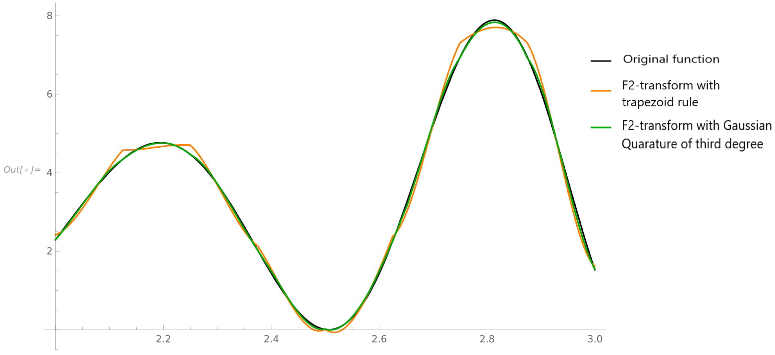
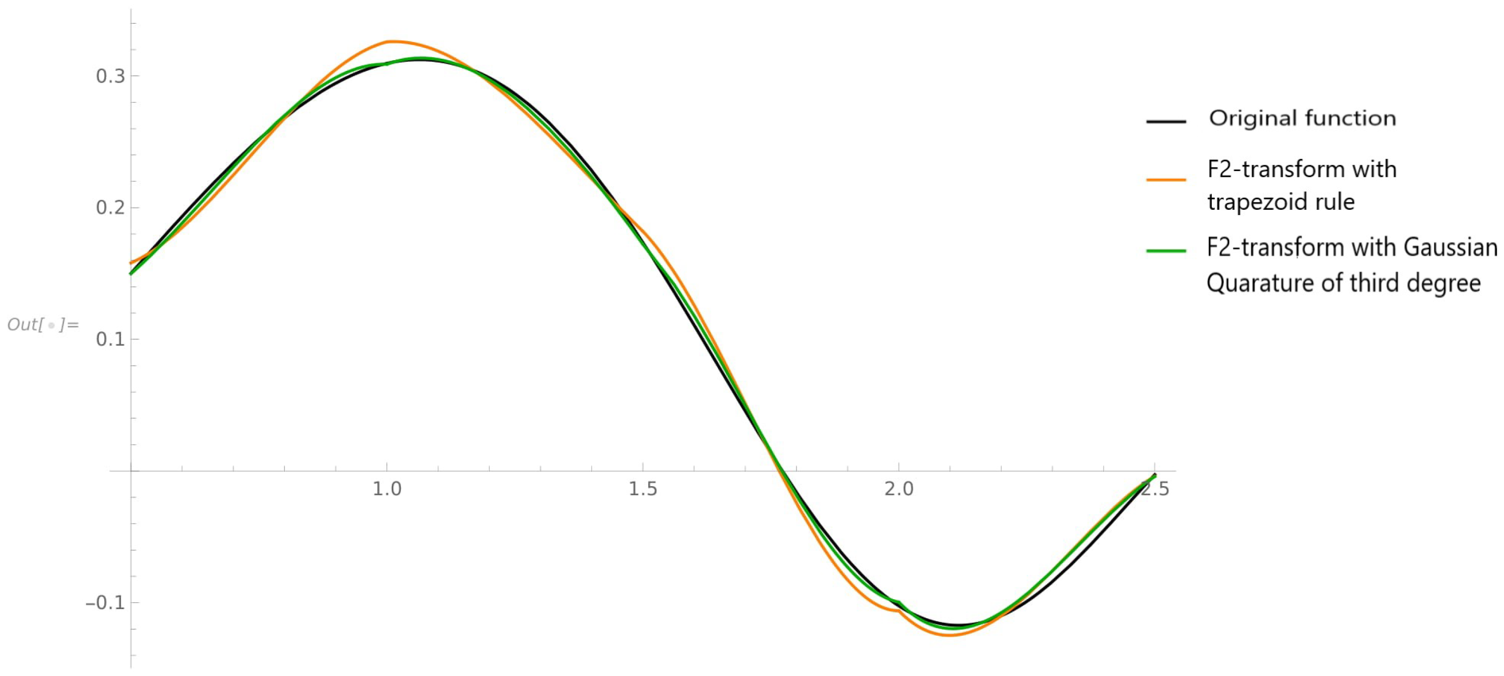
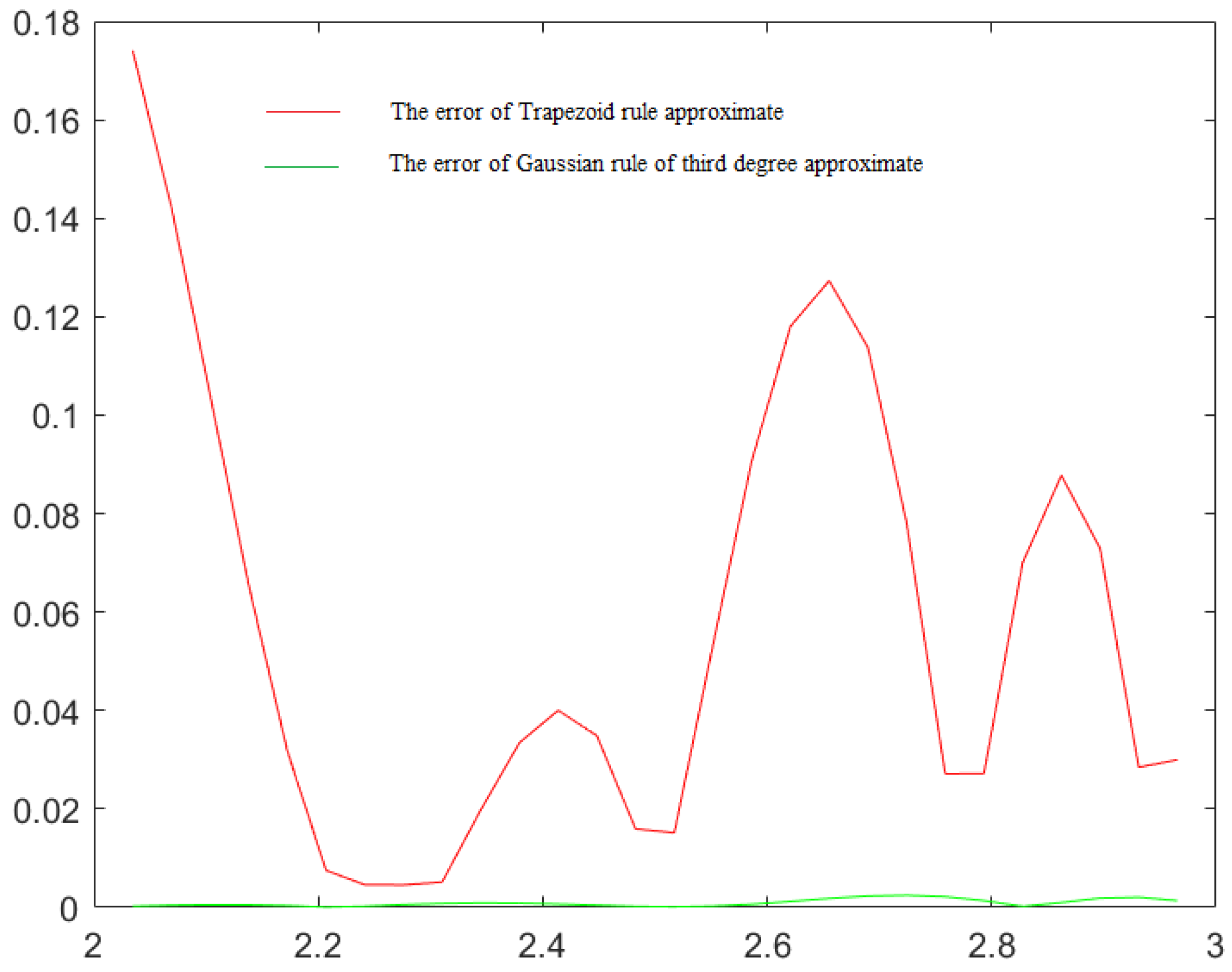
Remark 4.

It is worth noting that the proposed estimate in (59) is better than if we used the composite trapezoidal rule or Simpson’s rule (by [1], the order of estimation of the error of the composite Simpson rule is 4 vs. 6 in the proposed case) under the same conditions as for the (fuzzy) partition into sub-intervals of length h.

6. Numerical Tests

In this section, we show the usefulness of the Gaussian quadrature rules proposed above, defined by a new weight function and a new type of partitioning of the integration domain. Numerical tests were carried out to support two directions of scientific research: to reduce the complexity of calculating the components of the $F^m$-transform and its inverse, as well as to numerically substantiate a new method of numerical integration.

6.1. Towards Improving the Quality of Approximation by the Inverse $F^2$- and $F^3$-Transform

In all the examples in this subsection, the focus is on computing the inverse $F^m$-transform, where $m=2,3$, defined by a fuzzy partition with triangular basis functions. This problem is important for obtaining a good approximation using only algebraic functions. Since the calculation of the components of the $F^m$-transform is based on numerical integration, we use numerical methods and therefore we can evaluate their effectiveness by analyzing the quality of the approximation obtained by the inverse $F^m$-transforms.

In the examples below, we consider original functions with different smoothness characteristics and apply different quadrature rules to calculate the $F^m$-transform components. In all examples, we show that with the help of the proposed quadrature rules, a better quality of approximation can be achieved when compared with similar (in terms of the number of integration points) trapezoid rules and Gaussian quadratures based on Legendre or Chebyshev polynomials.

Example 2

(Smooth original function). In this example, we compute the inverse $F^2$-transform to approximate function $f\left(x\right)=\frac{sin{x}^2}{e^x}$ given in the domain $[0,2.5]$. For the computation of the components we use the composite trapezoid rule and the here proposed 3-point quadrature rule with the triangular weight functions $A_k$. Figure 1 shows the graphs of the original function and two corresponding inverse $F^2$-transforms. The error functions are presented in Figure 2 and show the obvious advantage of the proposed method.

Figure 1. Original function $f\left(x\right)=\frac{sin{x}^2}{e^x}$ and its two inverse $F^2$-transforms whose components were calculated using the trapezoid rule and the here proposed 3-point Gaussian quadrature rule.

Figure 2. Error functions of two approximations of the original function in Example 2, given by inverse $F^2$-transforms calculated using the trapezoid and the suggested quadratures. In the latter case, the errors are practically equal to zero.

Example 3.

(Slightly oscillatory original function) Similar to Example 2, we compute the inverse $F^2$-transform to approximate function $f\left(x\right)=x^2{(sin{x}^2)}^2$ given in the domain $[0,3]$. For the computation of the components we use the composite trapezoid rule and the here proposed 3- point quadrature rule with the triangular weight functions $A_k$. Figure 3 shows the graphs of the original function and two corresponding inverse $F^2$-transforms.

Figure 3. Original function $f\left(x\right)=x^2{(sin{x}^2)}^2$ and its two inverse $F^2$-transforms whose components were calculated using the trapezoid rule and the here proposed 3-point Gaussian quadrature rule.

The error functions are presented in Figure 4 and show an easily observable advantage of the proposed method.

Figure 4. Error functions of two approximations of the original function in Example 3, given by inverse $F^2$-transforms calculated using the trapezoid and the suggested quadratures. In the latter case, the errors are practically equal to zero.

Example 4

(Strongly oscillatory original function). Let $f\left(x\right)=sin{e}^{x^2}$ be considered in $[0,2]$. Because f oscillates strongly, the Newton–Cotes formulas based on equidistant points are inefficient [1]. Therefore, we increase the degree of the F-transform from 2 (previous examples) to 3 and perform calculations using 3 different four-point Gaussian quadrature rules based on Legendre, Chebyshev and the F-transform polynomials proposed here. Figure 5 shows the graphs of the original function and three corresponding inverse $F^3$-transforms. The error functions are presented in Figure 6 and as in the above examples, they show an easily observable advantage of the proposed method.

Figure 5. Original function $f\left(x\right)=sin{e}^{x^2}$ and its three inverse $F^3$-transforms whose components were calculated using the Legendre rule, Chebyshev and the here proposed 4-point Gaussian quadrature rule.

Figure 6. Error functions of three approximations of the original function in Example 4, given by inverse $F^3$-transforms calculated using the Legendre, Chebyshev and the suggested quadratures. In the latter case, the errors are zero almost everywhere.

6.2. Towards a New Method of Numerical Integration

Example 5.

This example confirms the results stated in Theorem 4. We use various Gaussian quadrature methods to approximate the integrals of functions with different smoothness. We consider three functions

$$\begin{array}{cc}\hfill f_1\left(t\right)& =|t-1|,t\in [0,2],\hfill \\ \hfill f_2\left(t\right)& =t^2{\left(sint\left(t^2\right)\right)}^2{A}_0(2t-1),t\in [0,1]\hfill \\ \hfill f_3\left(t\right)& =\left\{\begin{array}{cc}10\hfill & \mathrm{if}0\le t\le 2,\hfill \\ -1\hfill & \mathrm{if}2\le t\le 3,\hfill \end{array}\right.\hfill \end{array}$$

where $A_0\left(t\right)=1-\left|t\right|$.

Remark 5.

In the domains under consideration, the functions $f_1,f_2$ are non-differential, while the function $f_3$ is discontinuous.

In Table 1, we show the errors of the approximate values of the definite integrals calculated from the functions from Example 5 using various Gaussian methods in comparison with their exact values. We use the following abbreviations:

-

4 points quadrature rule with weight function $A_k$ (4.Gauss-FT).

-

3 points quadrature rule with weight function $A_k$ (3.Gauss-FT).

-

2 points Legendre method (2.Gauss-Leg).

-

3 points Legendre method (3.Gauss-Leg).

-

4 points Legendre method (4.Gauss-Leg).

-

5 points Legendre method (5.Gauss-Leg).

-

4 points Chebyshev method (4.Gauss-Cheb).

Table 1. The error estimates for various quadrature rules used in Example 5.

	Integrals	${\int }_0^2{\mathit{f}}_1\left(\mathit{t}\right)\mathbf{dt}$	${\int }_0^1{\mathit{f}}_2\left(\mathit{t}\right)\mathbf{dt}$	${\int }_0^3{\mathit{f}}_3\left(\mathit{t}\right)\mathbf{dt}$
Methods
4.Gauss-FT		0	4.0768 × 10−6	0
3.Gauss-FT		1.1102 × 10−16	2.3293 × 10−4	0.3208
2.Gauss-Leg		0.1547	0.0139	5.5
3.Gauss-Leg		0.1393	8.0056 × 10−4	1.8333
4.Gauss-Leg		0.042	1.3610 × 10−4	5.5
5.Gauss-Leg		0.0551	2.3937 × 10−4	0.8067
4.Gauss-Cheb		0.1107	0.0011	5.1467

Table 1. The error estimates for various quadrature rules used in Example 5.

	Integrals	${\int }_0^2{\mathit{f}}_1\left(\mathit{t}\right)\mathbf{dt}$	${\int }_0^1{\mathit{f}}_2\left(\mathit{t}\right)\mathbf{dt}$	${\int }_0^3{\mathit{f}}_3\left(\mathit{t}\right)\mathbf{dt}$
Methods
4.Gauss-FT		0	4.0768 × 10−6	0
3.Gauss-FT		1.1102 × 10−16	2.3293 × 10−4	0.3208
2.Gauss-Leg		0.1547	0.0139	5.5
3.Gauss-Leg		0.1393	8.0056 × 10−4	1.8333
4.Gauss-Leg		0.042	1.3610 × 10−4	5.5
5.Gauss-Leg		0.0551	2.3937 × 10−4	0.8067
4.Gauss-Cheb		0.1107	0.0011	5.1467

7. Conclusions

In this study, we focused on efficient numerical methods that we could use to calculate higher degree F-transform components. The latter are expressed as weighted orthogonal polynomials with weights given by fuzzy partition elements (basic functions) and coefficients (projections onto the corresponding polynomials) expressed using certain integrals. Therefore, in search of effective methods of numerical integration, we came to Gaussian quadrature rules, the accuracy of which depends on the number of integration points.

In this manuscript, we analyzed the 3- and 4-point Gaussian quadrature rules and found all their parameters, which allowed us to obtain exact analytical expressions for the values of certain integrals, in which the integrands are polynomials up to (inclusive) 7th degree. With their help, we have obtained good approximate estimates of the components of the $F^m$-transform for $m\le 3$, expressed without the use of definite integrals.

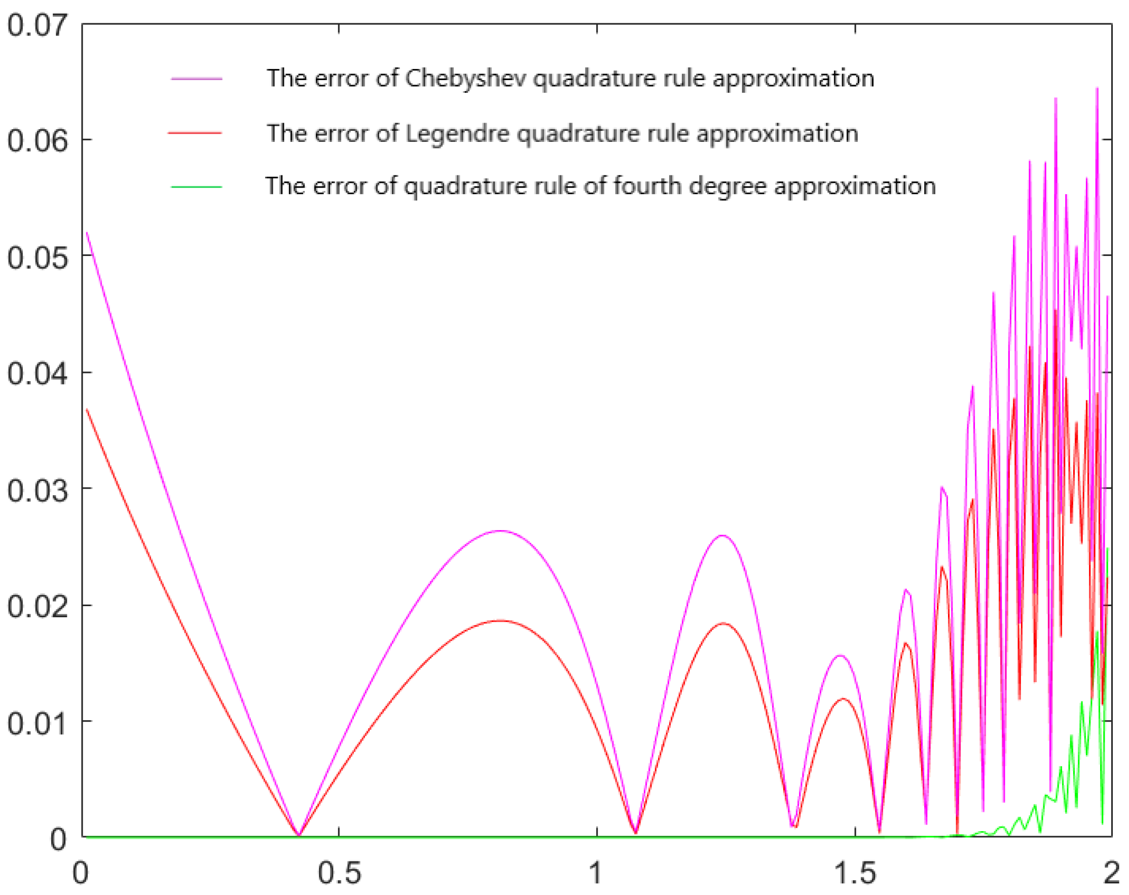
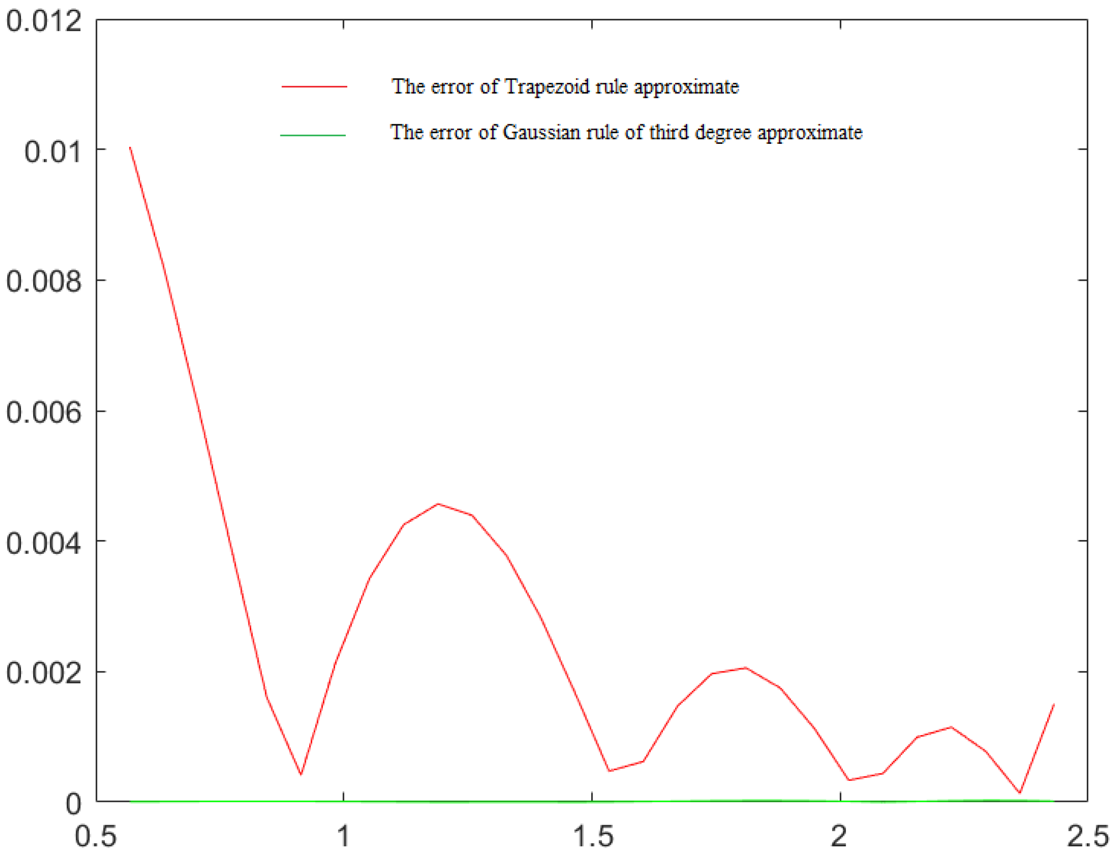
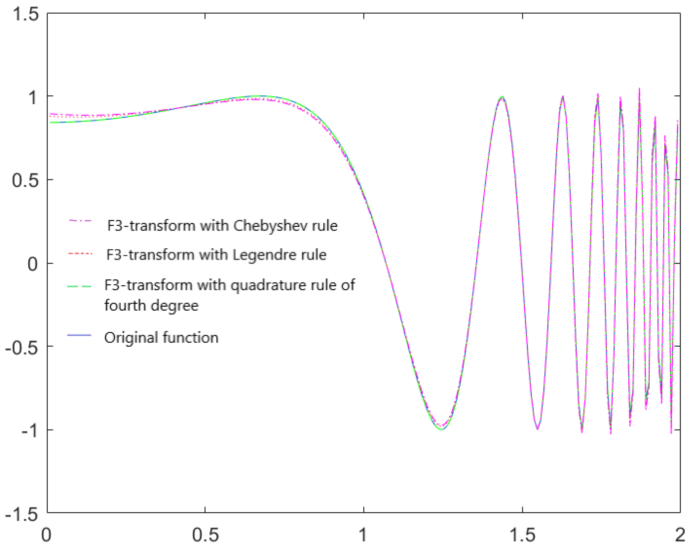
In addition, we have shown that our results can be useful for the numerical integration of arbitrary (integrable) functions. In this case, we gave an estimate of the error and compared it with the estimates of similar methods. We have shown that the approximation quality of the proposed method is at least two order better in comparison with the trapezoid and Simpson rules. We have compared our approach with other Gaussian quadrature rules, based on Legendre or Chebyshev polynomials. Finally, we performed numerical tests and confirmed all theoretical results.

In the future, we plan to use the received approximate estimates of the components of the $F^m$-transform for $m\le 3$, in all applications of F-transform methodology, where the main factors are accuracy and computational complexity. This includes numerical solutions of various differential and integral equations, processing images and time series.