Article

All Traveling Wave Exact Solutions of the Kawahara Equation Using the Complex Method

1
Department of Basic Courses Teaching, Software Engineering Institute of Guangzhou, Guangzhou 510990, China
2
School of statistics and Mathematics, Guangdong University of Finance and Economics, Guangzhou 510006, China
*
Authors to whom correspondence should be addressed.
Axioms 2022, 11(7), 330; https://doi.org/10.3390/axioms11070330
Submission received: 1 June 2022 / Revised: 28 June 2022 / Accepted: 29 June 2022 / Published: 7 July 2022
(This article belongs to the Special Issue Differential Equations and Genetic Algorithms)

Abstract

:
In this article, we prove that the p , q condition holds, first by using the Fuchs index of the complex Kawahara equation, and then proving that all meromorphic solutions of complex Kawahara equations belong to the class W. Moreover, the complex method is employed to get all meromorphic solutions of complex Kawahara equation and all traveling wave exact solutions of Kawahara equation. Our results reveal that all rational solutions u r ( x + ν t ) and simply periodic solutions u s , 1 ( x + ν t ) of Kawahara equation are solitary wave solutions, while simply periodic solutions u s , 2 ( x + ν t ) are not real-valued. Finally, computer simulations are given to demonstrate the main results of this paper. At the same time, we believe that this method is a very effective and powerful method of looking for exact solutions to the mathematical physics equations, and the search process is simpler than other methods.

1. Introduction and Main Results

In this article, we study all traveling wave exact solutions of the Kawahara equation [1]:
u t + a u u x + c u x x x d u x x x x x = 0 ,
where a , c , d are constants, x and t represent spatial and time variables, u u x is the nonlinear disturbance term, and u x x x and u x x x x x are the dispersion terms of order three and five, respectively. The solutions of Equation (1) could be used to analyze and interpret a lot of nonlinear dispersive phenomena that can arise in optical fiber, ocean, plasma physics, etc. [2,3]. Given the importance of this equation, it remains the subject of study for many researchers. Many different techniques were devoted to studying various solutions of Equation (1) and its family [4,5,6,7,8,9,10,11,12,13]. For example, Kudryashov [14], obtained exact meromorphic solutions of the Kawahara equation using the Laurent series. Wazwaz [15], found some different solutions (compacton and solitons) to Equation (1) in terms of trigonometric functions. Khan [16], analyzed the Kawahara equation using the variational approach and derived new conditions for obtaining solitary wave solutions. Using the traveling wave ansatz, Baiswas [17], studied the generalized Kawahara equation and derived a solitary wave solution for the family of the Kawahara equation. A lot of effective methods are applied to study the exact solutions, which makes the research more abundant [18,19,20,21,22,23]. Wang [24] used ansatz method to derive the exact solitary wave solution for the generalized Korteweg–de Vries–Kawahara (GKdV-K) equation. Aiman Zara [25] studied numerical approximation of the modified Kawahara equation using the Kernel smoothing method. El-Tantawy [26] derived a set of novel exact and approximate analytic solutions to the family of the forced damped Kawahara equation (KE) using the ansatz method.
In recent years, Yuan et al. [27,28] introduced the p , q condition to study a class of constant-coefficient complex algebraic differential equations with dominant terms, and obtained all possible meromorphic solutions which belong to the class W. That is to say, the general representation of rational function solutions, finitely growing simply periodic solutions and elliptic solutions, and both rational function solutions and simply periodic solutions can be obtained by degenerating elliptic general solutions. Futhermore, a complex method for obtaining exact solutions in the mathematical physics is presented. Using the complex method [27,28], we prove that all meromorphic solutions of complex Kawahara equation belong to the class W, and then get all meromorphic solutions of complex Kawahara equation and all traveling wave exact solutions of Equation (1). This method is simpler than other methods in the process of finding solutions, and can also be applied to the solution of other nonlinear differential equations.
Substitute the traveling wave transform
u = u ( x , t ) = w ( z ) , z = x + ν t
into Equation (1); integrate it to get
C 0 + ν w + 1 2 a w 2 + c w d w ( 4 ) = 0 ,
where C 0 is an integral constant.
Multiply Equation (3) by w , and integrate it; thus, we get the complex ordinary differential Kawahara equation
w w 1 2 ( w ) 2 A w 3 + B ( w ) 2 + C w 2 + D w + E = 0 ,
where A = a 6 d , B = c 2 d , C = ν 2 d , D = C 0 d , E = C 1 d , C 0 and C 1 are integral constants.
Now, we give the main results in our paper.
Theorem 1.
Let A 0 , then all meromorphic solutions w ( z ) of Equation (4) belong to the class W. Here, class W consists of elliptic functions and their degenerations with the form R ( z ) or R ( e α z ) , α C , where R is a rational function.
In addition, the solutions of Equation (4) have the forms:
(1) All elliptic function solutions
w d ( z ) = 35 2 A [ ( z ) + M ( z ) N ] 4 [ 140 ( ( z ) + N ) A 70 B 39 A ] [ ( z ) + M ( z ) N ] 2 + 280 A [ ( z ) + N ] 2 280 B 39 A [ ( z ) + N ] + C 3 A 62 B 2 1521 A 28 A g 2 ,
where g 3 = 31 B 3 593190 7 B 390 g 2 , M 2 = 4 N 3 g 2 N g 3 ,
g 2 2 2 B 2 507 g 2 + 1457 41384889 B 4 A D 1932 C 2 5796 = 0 ,
E = 1 A 2 [ ( 1148 69 A D + 1148 207 C 2 661248 656903 B 4 ) g 2 + 23808 4826809 B 6
+ ( 20 1521 A D + 20 4563 C 2 ) B 2 1 3 A C D 2 27 C 3 ] ,
D and N are constants.
(2) All simply periodic solutions
w s , 1 ( z ) = 2 B 2 169 A [ 35 coth 4 26 B i 26 ( z z 0 ) 70 coth 2 26 B i 26 ( z z 0 ) + 23 ] + C 3 A ,
and
w s , 2 ( z ) = B 2 507 A γ 2 [ 210 coth 4 B 26 γ ( z z 0 ) ( 140 γ + 560 ) coth 2 B 26 γ ( z z 0 ) + 166 γ + 352 ] + C 3 A ,
where z 0 C ; D = 1 85683 5184 B 4 28561 C 2 A ,
E = 1 130323843 746496 B 6 2628288 B 4 C + 4826809 C 3 A 2
in w s , 1 ( z ) , and
D = 1 23905557 ( 217620 γ 59724 ) B 4 γ 4 A C 2 3 A ,
E = 1 A 2 [ 16 B 6 448893237 3001 7007 γ γ 6 B 4 C 71716671 217620 γ 59724 γ 4 + C 3 27 ] ,
γ is a root of 31 z 2 31 z + 10 = 0 in w s , 2 ( z ) .
(3) All rational function solutions
w r ( z ) = 280 A 1 ( z z 0 ) 4 + C 3 A ,
where B = 0 , D = C 2 3 A , E = C 3 27 A 2 and z 0 C .
All traveling wave exact solutions of Equation (1) are obtained by substituting (2) into meromorphic solutions w of Equation (4). So, we get the following Theorem.
Theorem 2.
Let a d 0 , all traveling wave exact solutions u ( x , t ) of Equation (1) have the following forms:
(1) All elliptic function solutions
u d ( x + ν t ) = 105 d a [ ( x + ν t ) + M ( x + ν t ) N ] 4 ( 840 d ( ( x + ν t ) + N ) a + 70 c 13 a ) [ ( x + ν t ) + M ( x + ν t ) N ] 2 + 1680 d a [ ( x + ν t ) + N ] 2 + 280 c 13 a [ ( x + ν t ] + N ) 168 d a g 2 31 c 2 507 a d ν a ,
where M 3 = 4 N 3 g 2 N g 3 , g 3 = 31 c 3 4745520 d 3 + 7 c 780 d g 2 ,
g 2 2 c 2 1014 d 2 g 2 + 1457 c 4 662158224 d 4 + a C 0 11592 d 2 ν 2 23184 d 2 = 0 ,
and C 0 , N are constants.
(2) All simply periodic solutions
u s , 1 ( x + ν t ) = 3 c 2 169 a d [ 35 coth 4 ( 1 2 c 13 d ( x x 0 + ν ( t t 0 ) ) ) 70 coth 2 ( 1 2 c 13 d ( x x 0 + ν ( t t 0 ) ) ) + 23 ] ν a ,
and
u s , 2 ( x + ν t ) = c 2 338 a d γ 2 [ 210 coth 4 ( 1 2 c 13 d γ ( x x 0 + ν ( t t 0 ) ) ) ( 140 γ + 560 ) coth 2 ( 1 2 c 13 d γ ( x x 0 + ν ( t t 0 ) ) ) + 166 γ + 352 ] ν a ,
where γ is a root of 31 z 2 31 z + 10 = 0 .
(3) All rational function solutions
u r ( x + ν t ) = 1680 d a 1 ( x x 0 + ν ( t t 0 ) ) 4 ν a ,
where c = 0 , x 0 and t 0 are arbitrary real constants.
The rest of the article is organized in the following order: In Section 2, we will present the relevant lemmas and methodology. Section 3 gives the detailed proof process of Theorem 1 and concise proof method of Theorem 2. Section 4 illustrates our main results using computer simulations. In the last section, some conclusions are given.

2. Preliminary Lemmas and the Complex Method

We need some definitions and lemmas in order to prove Theorem 1 and present the complex method.
Set k , n N : = { 1 , 2 , 3 , . . . } , r j N 0 = N { 0 } , r = ( r 0 , r 1 , . . . , r k ) , j = 0 , 1 , . . . , k .
M r [ w ] ( z ) : = [ w ( z ) ] r 0 [ w ( z ) ] r 1 [ w ( z ) ] r 2 [ w ( k ) ( z ) ] r k .
The degree of M r [ w ] defined by d ( r ) : = r 0 + r 1 + + r k .
Definition 1 ([28]).
A differential polynomial is defined by
P [ w ] : = r Λ b r M r [ w ] ,
where Λ is a finite index set, and b r are constants. deg P [ w ] : = max r Λ { d ( r ) } is called the degree of P [ w ] .
Consider the differential equation
E ( z , w ) : = P [ w ] a w n = 0 ,
where a 0 is a constant.
The dominant part of E ( z , w ) composes all dominant terms which can determine the multiplicity q of w in E ( z , w ) , and is denoted by E ^ ( z , w ) . D ( q ) and D r ( q ) represent the multiplicity of pole of each term in E ^ ( z , w ) and the multiplicity of pole of each monomial in E ( z , w ) E ^ ( z , w ) , respectively.
Obviously
D r ( q ) = q d ( r ) + r 1 + 2 r 2 + + k r k < D ( q ) .
Definition 2 ([28]).
The derivative of E ^ ( z , w ) with respect to w can be calculated by the following formula, for any χ ,
E ^ ( z , w ) χ = lim λ 0 E ^ ( z , w + λ χ ) E ^ ( z , w ) λ .
Definition 3 ([28]).
Substituting Laurent series
w ( z ) = l = q c l z l ,
into Equation (15), where c q 0 , q > 0 . Then, we can get p different principle
l = q 1 c l z l
with pole of multiplicity q at z = 0 , Equation (15) is said to satisfy weak p , q condition. If Equation (15) has p different meromorphic solutions with pole of multiplicity q at z = 0 , Equation (15) satisfies p , q condition.
Definition 4 ([28]).
Let T 1 , T 2 be two given complex numbers, such that I m T 1 T 2 > 0 , L = L [ 2 T 1 , 2 T 2 ] is discrete subset L [ 2 T 1 , 2 T 2 ] = { T | T = 2 m T 1 + 2 n T 2 , m , n Z } , which is isomorphic to Z × Z . The discriminant Δ = Δ ( c 1 , c 2 ) : = c 1 3 27 c 2 2 and
s n = s n ( L ) : = T L \ { 0 } 1 T n .
Weierstrass elliptic function ( z ) : = ( z , g 2 , g 3 ) is a meromorphic function with double periods 2 T 1 , 2 T 2 , which satisfies the following formula
( ( z ) ) 2 = 4 ( z ) 3 g 2 ( z ) g 3 ,
where g 2 = 60 s 4 , g 3 = 140 s 6 and Δ ( g 2 , g 3 ) 0 .
Definition 5 ([29]).
The Fuchs index of Equation (15) can be defined as the root of the equation
P ( i ) = lim z 0 z i + D ( q ) E ^ ( z , c q z q ) z i q = 0
Lemma 1 ([28,30,31,32]).
Set p , q , m , n N , deg P [ w ] < n . If Equation (15) satisfies p , q condition, all meromorphic solutions w ( z ) of Equation (15) belong to class W.
Any elliptic function solution with pole at z = 0 is given in the form
w ( z ) = i = 1 m 1 j = 2 q ( 1 ) j c i j ( j 1 ) ! d j 2 d z j 2 ( 1 4 [ ( z ) + M i ( z ) N i ] 2 ( z ) ) + i = 1 m 1 c i 1 2 ( z ) + M i ( z ) N i + j = 2 q ( 1 ) j c m j ( j 1 ) ! d j 2 d z j 2 ( z ) + k 0 ,
where c i j can be determined by (18), c i j and k 0 are constants. M i 2 = 4 N i 3 g 2 N i g 3 and i = 1 m c i 1 = 0 .
Any rational function solution w : = R ( z ) is expressed as
R ( z ) = i = 1 m j = 1 q c i j ( z z i ) j + k 0 ,
which has m ( p ) different poles of multiplicity q.
Any simply periodic solution w : = R ( ξ ) is a rational function of ξ = e α z ( α C ) and can be given in the form
R ( ξ ) = i = 1 m j = 1 q c i j ( ξ ξ i ) j + k 0 ,
which has m ( p ) different poles of multiplicity q.
Lemma 2 ([33,34]).
Weierstrass elliptic functions ( z ) have the addition formula and two successive degeneracies, as shown below:
(I) Addition formula
( z z 0 ) = ( z ) ( z 0 ) + 1 4 [ ( z ) + ( z 0 ) ( z ) ( z 0 ) ] 2 .
(II) If Δ ( g 2 , g 3 ) = 0 , Weierstrass elliptic functions degenerate to simply periodic functions, which can be expressed as
( z , 3 δ 2 , δ 3 ) = 2 δ 3 δ 2 coth 2 3 δ 2 z .
(III) If g 2 = g 3 = 0 , Weierstrass elliptic functions degenerate to rational functions of z, which can be expressed as
( z , 0 , 0 ) = 1 z 2 .
Next, we give the complex method.
  • Substituting the transform T : u ( x , t ) w ( z ) , ( x , t ) z into a given PDE yields a nonlinear ODE: Equation (4) here.
  • Insert (18) into Equation (4) here to determine that weak p , q condition holds.
  • By (22)–(24), we obtain all meromorphic solutions w ( z ) of Equation (4) here with pole at z = 0 .
  • Get all meromorphic solutions w ( z z 0 ) by Lemmas 1 and 2.
  • Inserting the inverse transform T 1 into w ( z z 0 ) , we obtain all exact solutions u ( x , t ) of the given partial differential equation.

3. Proof of Theorem 1

From balance the order of the poles in Equation (4), yields
( q + 1 ) + ( q + 3 ) = 2 ( q + 2 ) = 3 q ,
and we get q = 4 .
Substitute (18) into Equation (4),and set the cofficients to zero, we have
c 4 = 280 A , c 3 = 0 , c 2 = 280 B 39 A , c 1 = 0 ,
c 0 = 62 B 2 507 C 1521 A , c 1 = 0 , c 2 = 62 B 3 59319 A , c 3 = 0 ,
c 4 = 1 425673144 11780 B 4 + 257049 A D + 85683 C 2 A , .
and then determine p = 1 . Therefore, Equation (4) is said to satisfy weak 1 , 4 condition. We also get that all meromorphic solutions of Equation (4) belong to W if Equation (4) satisfies 1 , 4 condition by Lemma 1.
In fact, since (17) and E ^ ( z , w ) = w w 1 2 ( w ) 2 A w 3 of Equation (4), we have D ( 4 ) = 12 ,
D r ( 4 ) < 12 , A c 4 = 280 ,
and
E ^ ( x , c 4 x 4 ) x i 4 = ( ( c 4 x 4 ) d 3 d x 3 + ( c 4 x 4 ) d d x ( c 4 x 4 ) d 2 d x 2 3 A ( c 4 x 4 ) 2 ) x i 4 = 4 ( i 1 ) ( i 4 ) ( i 5 ) + 120 i + 360 c 4 x i 12 .
Thus, from (29), (30) and (21), we infer that the Fuchs index of Equation (4) are zeros of the function
P ( i ) = 4 ( i 1 ) ( i 4 ) ( i 5 ) + 120 i + 360 c 4 .
It is easy to prove that f ( x ) : = 4 ( x 1 ) ( x 4 ) ( x 5 ) + 120 x + 360 > 0 if x > 1 . Hence, if i N , then P ( i ) 0 . That is to say, the Fuchs index of Equation (4) cannot be a positive integer. This implies that (ref. [29], p. 90): The principle part of the Laurent series of w ( z ) determines the whole Laurent series of w ( z ) . Therefore, weak 1 , 4 condition implies that 1 , 4 condition holds.
From, (23), we get the indeterminant form of rational function solutions of Equation (4) at pole z = 0
R 1 ( z ) = c 4 z 4 + c 2 z 2 + k 0 = 280 A 1 z 4 + 280 B 39 A 1 z 2 + k 0 .
Inserting (32) into Equation (4), and then setting the coefficients to zero, we get the system of Equations (1) which are given in Appendix A. Computing the system of Equations (1), we get
k 0 = C 3 A , B = 0 , D = C 2 3 A , E = C 3 27 A 2 .
So we find that the rational function solutions of Equation (4) are
w r 0 ( z ) = 280 A 1 z 4 + C 3 A ,
at pole z = 0 , here B = 0 , D = C 2 3 A , E = C 3 27 A 2 .
Hence, all rational function solutions of Equation (4) are
w r ( z ) = 280 A 1 ( z z 0 ) 4 + C 3 A ,
where B = 0 , D = C 2 3 A , E = C 3 27 A 2 and z 0 C .
By (22) and (26), we get the indeterminant form of simply periodic solutions of Equation (4) at pole z = 0
w s 0 ( z ) = 1 6 c 4 ( z , 3 δ 2 , δ 3 ) + c 2 ( z , 3 δ 2 , δ 3 ) + k 0 = 280 6 A ( z , 3 δ 2 , δ 3 ) + 280 B 39 A ( z , 3 δ 2 , δ 3 ) + k 0 ,
where ( z , 3 δ 2 , δ 3 ) = 2 δ 3 2 δ coth 2 3 δ 2 z .
Expanding ( z , 3 δ 2 , δ 3 ) at z 0 = 0 , we have
( z , 3 δ 2 , δ 3 ) = 1 z 2 + 3 δ 2 20 z 2 δ 3 28 z 4 + o ( z 4 )
Substituting (36) into (35), we get
w ( z ) = 280 A 1 z 4 + 280 B 39 A 1 z 2 + 14 δ 2 A + k 0 + ( 14 B δ 2 13 A 20 δ 3 A ) z 2 + ( 10 B δ 3 39 A + 21 δ 4 2 A ) z 4 + o ( z 4 )
Comparing coefficients of (37) and (28), we obtain the system of Equations (2) which are showed in Appendix A. Solving the system of Equations (2), we have
δ = B 39 , k 0 = 76 B 2 1521 A + C 3 A , D = 1 85683 5184 B 4 28561 C 2 A ,
and
δ = B 39 γ , k 0 = B 2 1521 A 6 62 γ γ 2 + C 3 A ,
D = 1 23905557 ( 217620 γ 59724 ) B 4 γ 4 A C 2 3 A . .
Substituting (35), (38) and (39) into Equation (4), from the correlation of coefficients we can obtain, respectively,
E = 1 130323843 746496 B 6 2628288 B 4 C + 4826809 C 3 A 2
and
E = 1 A 2 [ 16 B 6 448893237 3001 7007 γ γ 6 B 4 C 71716671 217620 γ 59724 γ 4 + C 3 27 ] ,
where γ is a root of 31 z 2 31 z + 10 = 0 .
Hence, we obtain the simply periodic solutions of Equation (4) at pole z = 0 are
w s , 1 ( z ) = 2 B 2 169 A [ 35 coth 4 26 B i 26 z 70 coth 2 26 B i 26 z + 23 ] + C 3 A ,
and
w s , 2 ( z ) = B 2 507 A γ 2 [ 210 coth 4 B 26 γ z ( 140 γ + 560 ) coth 2 B 26 γ z + 166 γ + 352 ] + C 3 A ,
where δ = B 39 , k 0 = 76 B 2 1521 A + C 3 A , D = 1 85683 5184 B 4 28561 C 2 A ,
E = 1 130323843 746496 B 6 2628288 B 4 C + 4826809 C 3 A 2
in w s , 1 ( z ) , and D = 1 23905557 ( 217620 γ 59724 ) B 4 γ 4 A C 2 3 A ,
E = 1 A 2 [ 16 B 6 448893237 3001 7007 γ γ 6 B 4 C 71716671 217620 γ 59724 γ 4 + C 3 27 ] ,
γ is a root of 31 z 2 31 z + 10 = 0 in w s , 2 ( z ) .
Furthermore, all simply periodic solutions of Equation (4) are given by
w s , 1 ( z ) = 2 B 2 169 A [ 35 coth 4 26 B i 26 ( z z 0 ) 70 coth 2 26 B i 26 ( z z 0 ) + 23 ] + C 3 A ,
and
w s , 2 ( z ) = B 2 507 A γ 2 [ 210 coth 4 B 26 γ ( z z 0 ) ( 140 γ + 560 ) coth 2 B 26 γ ( z z 0 ) + 166 γ + 352 ] + C 3 A ,
where z 0 C , D = 1 85683 5184 B 4 28561 C 2 A ,
E = 1 130323843 746496 B 6 2628288 B 4 C + 4826809 C 3 A 2
in w s , 1 ( z ) , and D = 1 23905557 ( 217620 γ 59724 ) B 4 γ 4 A C 2 3 A ,
E = 1 A 2 [ 16 B 6 448893237 3001 7007 γ γ 6 B 4 C 71716671 217620 γ 59724 γ 4 + C 3 27 ] ,
γ is a root of 31 z 2 31 z + 10 = 0 in w s , 2 ( z ) .
From (22), we infer the indeterminant forms of elliptic function solutions of Equation (4) are
w d 0 ( z ) = c 4 6 ( z ) + c 2 ( z ) + k 0 = 280 6 A + 280 B 39 A + k 0 .
with pole at z = 0 .
Expanding ( z , g 2 , g 3 ) at z = 0 , we have
( z , g 2 , g 3 ) = 1 z 2 + g 2 20 z 2 + g 3 28 z 4 + o ( z 4 ) .
Put (45) into (44) and apply (20), we get
w ( z ) = 280 A 1 z 4 + 280 B 39 A 1 z 2 + 14 g 2 3 A + k 0 + ( 14 B g 2 39 A + 20 g 3 A ) z 2 + ( 10 B g 3 39 A + 7 g 2 2 6 A ) z 4 + o ( z 4 ) .
Comparing coefficients of w ( z ) and (28), we obtain the system of Equations (3). which are shown in the Appendix. Computing the system of Equations (3), we derive
k 0 = C 3 A 14 3 A g 2 62 B 2 1521 A , g 3 = 31 B 3 593190 7 B 390 g 2 .
and g 2 satisfies
g 2 2 2 B 2 507 g 2 + 1457 B 4 41384889 A D 1932 C 2 5796 = 0 .
Substituting (44) and (47) into Equation (4), from the correlation of coefficients, we can get
E = 1 A 2 { ( 1148 69 A D + 1148 207 C 2 661248 656903 B 4 ) g 2 + 23808 4826809 B 6 + ( 20 1521 A D + 20 4563 C 2 ) B 2 1 3 A C D 2 27 C 3 } ,
then we have
w d 0 ( z ) = 280 A 2 ( z ) + 280 B 39 A ( z ) + C 3 A 62 B 2 1521 A 28 A g 2 .
Thus, all elliptic function solutions of Equation (4) are
w d ( z ) = 280 A 2 ( z z 0 ) + 280 B 39 A ( z z 0 ) + C 3 A 62 B 2 1521 A 28 A g 2 ,
where z 0 C , g 3 = 31 B 3 593190 7 B 390 g 2 ,
E = 1 A 2 { ( 1148 69 A D + 1148 207 C 2 661248 656903 B 4 ) g 2 + 23808 4826809 B 6 + ( 20 1521 A D + 20 4563 C 2 ) B 2 1 3 A C D 2 27 C 3 } ,
and g 2 satisfies
g 2 2 2 B 2 507 g 2 + 1457 B 4 41384889 A D 1932 C 2 5796 = 0 .
By using the addition formula, we can get another representation of it as
w d ( z ) = 35 2 A [ ( z ) + M ( z ) N ] 4 [ 140 ( ( z ) + N ) A 70 B 39 A ] [ ( z ) + M ( z ) N ] 2 + 280 A [ ( z ) + N ] 2 280 B 39 A [ ( z ) + N ] + C 3 A 62 B 2 1521 A 28 A g 2 ,
where
M 2 = 4 N 3 g 2 N g 3 , g 3 = 31 B 3 593190 7 B 390 g 2 ,
g 2 2 2 B 2 507 g 2 + 1457 41384889 B 4 A D 1932 C 2 5796 = 0 ,
E = 1 A 2 [ ( 1148 69 A D + 1148 207 C 2 661248 656903 B 4 ) g 2 + 23808 4826809 B 6
+ ( 20 1521 A D + 20 4563 C 2 ) B 2 1 3 A C D 2 27 C 3 ] ,
D and N are constants.
So far, we have completed the proof of Theorem 1.
Substituting (2) into all meromorphic solutions w ( z ) of Equation (4), we obtained Theorem 2. According to the theorem in ref. [35], we can get the following corollary.
Corollary. All rational solutions u r ( x + ν t ) and simply periodic solutions u s , 1 ( x + ν t ) of Equation (1) are real valued, while simply periodic solutions u s , 2 ( x + ν t ) are not real valued.

4. Computer Simulations

This subsection will show our results through computer simulations of u r ( x + ν t ) and u s , 1 ( x + ν t ) , as demonstrated in the following figures.
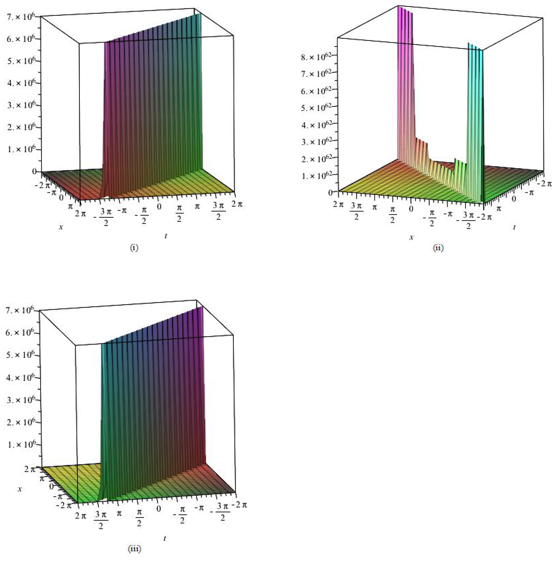
  • By applying the complex method, we are able to achieve the rational solution u r ( x + ν t ) of Equation (4). Figure 1 describes the 3D graphs of solution u r ( x + ν t ) for a = 1 , ν = 1 , and d = 1 1680 within the interval 5 x , t 5 . Figure 2 shows the 2D graphs of solution u r ( x + ν t ) for a = 1 , ν = 1 , and d = 1 1680 within the interval 10 x 10 when t = 0 . It could be observed that they have one generation pole, which is shown by Figure 1 and Figure 2.
  • By employing the complex method, we are able to obtain the simply periodic solutions u s , 1 ( x + ν t ) and u s , 2 ( x + ν t ) of Equation (4). Figure 3 shows the 3D graphs of solution u s , 1 ( x + ν t ) for a = 3 , c = 13 , d = 1 , and ν = 3 within the interval 2 π x , t 2 π . Figure 4 describes the 2D graphs of solution u s , 1 ( x + ν t ) for a = 3 , c = 13 , d = 1 , and ν = 3 within the interval 2 π x 2 π when t = 0 .

5. Conclusions

In this paper, we are the first to utilize the complex method to prove that all meromorphic solutions of complex Kawahara equation belong to the class W, and then we get all meromorphic solutions of complex Kawahara equation and all traveling wave exact solutions of Equation (1). In addition, we find that all rational solutions u r ( x + ν t ) and simply periodic solutions u s , 1 ( x + ν t ) of Equation (1) are solitary wave solutions, which could be used to analyze and interpret a lot of nonlinear dispersive phenomena. This research enriches the methods of solving differential equations. Our results also reveal that the complex method of looking for traveling wave exact solutions is general and feasible, and can be applied to other nonlinear partial differential equations.

Author Contributions

Conceptualization, J.T. and Y.G.; methodology, J.T. and Y.G.; software, C.J.; writing—original draft, F.Y. and X.Z.; writing—review, editing, T.O. All authors have read and agreed to the published version of the manuscript.

Funding

This work is supported by the NSF of China (11901111), Young Innovative Talents Project of Guangdong Universities (2021KQNCX130), Science Research Group Project of SEIG (ST202101).

Institutional Review Board Statement

Not applicable.

Informed Consent Statement

Not applicable.

Data Availability Statement

Not applicable.

Acknowledgments

The authors would like to express their hearty thanks to the editor and referees for their very helpful comments and useful suggestions.

Conflicts of Interest

The authors declare no conflict of interest.

Appendix A

  • The system of Equations (1):
    A k 0 3 + C k 0 2 + D k 0 + E = 0 ,
    280 13 B k 0 2 + 560 39 B C A k 0 + 280 B D 39 A = 0 ,
    840 k 0 2 + ( 560 C A 78400 B 2 507 A ) k 0 + 78400 B 2 C 1521 A 2 + 280 D A = 0 ,
    156800 B 13 A k 0 9721600 B 3 59319 A 2 + 156800 B C 39 A 2 = 0 ,
    235200 A k 0 4860800 B 2 507 A 2 + 78400 C A 2 = 0 .
  • The system of Equations (2):
    14 δ 2 A + k 0 = 62 B 2 507 C 1521 A ,
    14 B δ 2 13 A 20 δ 3 A = 62 B 3 59319 A ,
    10 B δ 3 39 A + 21 δ 4 2 A = 11780 B 4 + 257049 A D + 85683 C 2 425673144 .
  • The system of Equations (3):
    14 g 2 3 A + k 0 = 62 B 2 507 C 1521 A ,
    14 B g 2 39 A + 20 g 3 A = 62 B 3 59319 A ,
    10 B g 3 39 A + 7 g 2 2 6 A = 11780 B 4 + 257049 A D + 85683 C 2 425673144 .

References

  1. Kawahara, T. Oscillatory solitary waves in dispersive media. J. Phys. Soc. Jpn. 1972, 33, 260–264. [Google Scholar] [CrossRef]
  2. Wazwaz, A.M. New solitary wave solutions to the Kuramoto-Sivashinsky and the Kawahara equations. Appl. Math. Comput. 2006, 182, 1642–1650. [Google Scholar] [CrossRef]
  3. Yusufoǧlu, E.; Bekir, A.; Alp, M. Periodic and solitary wave solutions of Kawahara and modified Kawahara equations by using sine-cosine method. Chaos. Soliton. Fract. 2008, 37, 1193–1197. [Google Scholar] [CrossRef]
  4. Kaya, D.; Al-Khaled, K. A numerical comparison of a Kawahara equation. Phys. Lett. A. 2007, 363, 433–439. [Google Scholar] [CrossRef]
  5. Wazwaz, A.M. Partial Differential Equations and Solitary Waves Theory; Higher Education Press: Beijing, China, 2009. [Google Scholar]
  6. Jang, B. New exact travelling wave solutions of Kawahara type equations. Nonlinear Anal. 2009, 70, 510–515. [Google Scholar] [CrossRef]
  7. Kudryashov, N.A. A note on new exact solutions for the Kawahara equation using exp-function method. J. Comput. Appl. Math. 2010, 234, 3511–3512. [Google Scholar] [CrossRef] [Green Version]
  8. Kaur, L.; Gupta, R.K. Kawahara equation and modified Kawahara equation with time dependent coefficients: Symmetry analysis and generalized (G’/G)- expansion method. Math. Methods Appl. Sci. 2012, 36, 584–600. [Google Scholar] [CrossRef]
  9. Pinar, Z.; Öziş, Z.T. The periodic solutions to Kawahara equation by means of the auxiliary equation with a sixth-degree nonlinear term. J. Math. 2013, 2013, 106349. [Google Scholar] [CrossRef] [Green Version]
  10. Mahmood, B.A.; Yousif, M.A. A novel analytical solution for the modified Kawahara equation using the residual power series method. Nonlinear Dyn. 2017, 89, 1233–1238. [Google Scholar] [CrossRef]
  11. El-Tantawy, S.A.; Salas, A.H.; Alharthi, M.R. Novel analytical cnoidal and solitary wave solutions of the extended Kawahara equation. Chaos. Soliton. Fract. 2021, 147, 110965. [Google Scholar] [CrossRef]
  12. Ghanbari, B.; Kumar, S.; Niwas, M.; Baleanu, D. The life symmetry analysis and exact Jacobi elliptic solutions for the Kawahara-KDV type equations. Results. Phys. 2021, 23, 104006. [Google Scholar] [CrossRef]
  13. Dascioǧlu, A.; Cuiha, S. Unal New exact solutions for the space-time fractional Kawahara equation. Appl. Math. Model. 2021, 89, 952–965. [Google Scholar] [CrossRef]
  14. Demina, M.V.; Kudryashov, N.A. From Laurent series to exact meromorphic solutions: The Kawahara equation. Phys. Lett. A. 2010, 374, 4023–4029. [Google Scholar] [CrossRef] [Green Version]
  15. Wazwaz, A.M. Compacton solutions of the Kawahara-type nonlinear dispersive equation. Appl. Math. Comput. 2003, 145, 133–150. [Google Scholar] [CrossRef]
  16. Khan, Y. A new necessary condition of soliton solutions for Kawahara equation arising in physics. Optik 2018, 155, 273–275. [Google Scholar] [CrossRef]
  17. Biswas, A. Solitary wave solution for the generalized Kawahara equation. Appl. Math. Lett. 2009, 22, 208–210. [Google Scholar] [CrossRef] [Green Version]
  18. Khan, K.; Akbar, M. The exp(-ϕ(ξ))-expansion method for finding traveling wave solutions of Vakhnenko-Parkes equation. Int. J. Dyn. Syst. Differ. Equ. 2014, 5, 72–83. [Google Scholar]
  19. Khan, K.; Akbar, M.; Koppelaar, H. Study of coupled nonlinear partial differential equations for finding exact analytical solutions. R. Soc. Open Sci. 2015, 2, 140406. [Google Scholar] [CrossRef] [Green Version]
  20. Jafari, H.; Kadkhoda, N.; Baleanu, D. Fractional Lie group method of the time-fractional Boussinesq equation. Nonlinear Dyn. 2015, 81, 1569–1574. [Google Scholar] [CrossRef]
  21. Jafari, H.; Kadkhoda, N.; Azadi, M.; Yaghoubi, M. Group classification of the time-fractional Kaup-Kupershmidt equation. Sci. Iran. 2017, 24, 302–307. [Google Scholar] [CrossRef] [Green Version]
  22. Sahoo, S.; Ray, S. Solitary wave solutions for time fractional third order modified kdv equation using two reliable techniques G’/G-expansion method and improved G’/G-expansion method. Phys. Lett. A 2010, 374, 4023–4029. [Google Scholar] [CrossRef]
  23. Özkan, E.M.; Özkan, A. The soliton solutions for some nonlinear fractional differential equations with Beta-derivative. Axioms 2021, 10, 203. [Google Scholar] [CrossRef]
  24. Wang, X.F.; Cheng, H. Solitary wave solution and a linear mass-conservative difference scheme for the generalized Korteweg-de Vries Kawahara equation. Comput. Appl. Math. 2021, 40, 273. [Google Scholar] [CrossRef]
  25. Rehman, S.U.; Ahmad, F.; Kouser, S.; Pervaiz, A. Numerical approximation of modified Kawahara equation using Kernel smoothing method. Math. Comput. Simul. 2022, 194, 169–184. [Google Scholar]
  26. El-Tantawy, S.A.; Salas, A.H.; Alyousef, H.A.; Alharthi, M.R. Novel exact and approximate solutions to the family of the forced damped Kawahara equation and modeling strong nonlinear waves in a plasma. Chin. J. Phys. 2022, 77, 2454–2471. [Google Scholar] [CrossRef]
  27. Yuan, W.J.; Li, Y.Z.; Lin, J.M. Meromorphic solutions of an auxiliary ordinary differential equation using complex method. Math. Method Appl. Sci. 2013, 36, 1776–1782. [Google Scholar] [CrossRef]
  28. Yuan, W.J.; Wu, Y.H.; Chen, Q.H.; Huang, Y. All meromorphic solutions for two forms of odd order algebraic differential eqyations and its applications. Appl. Math. Comput. 2014, 240, 240–251. [Google Scholar]
  29. Conte, R. The Painlevé approach to nonlinear ordinary differential equations. In The Painlev Property, One Century Later, CRM Series in Mathematical Physics; Conte, R., Ed.; Springer: New York, NY, USA, 1999; pp. 77–180. [Google Scholar]
  30. Yuan, W.J.; Huang, Y.; Shang, Y.D. All travelling wave exact solutions of two nonlinear physical models. Appl. Math. Comput. 2013, 219, 6212–6223. [Google Scholar]
  31. Yuan, W.J.; Shang, Y.D.; Huang, Y.; Wang, H. The representation of meromorphic solutions of certain ordinary differential equations and its applications. Sci. Sin. Math. 2013, 43, 563–575. [Google Scholar]
  32. Yuan, W.J.; Meng, F.N.; Huang, Y.; Wu, Y.H. All traveling wave exact solutions of the variant Boussinesq equations. Appl. Math. Comput. 2015, 268, 865–872. [Google Scholar] [CrossRef]
  33. Lang, S. Elliptic Functions, 2nd ed.; Springer: New York, NY, USA, 1987. [Google Scholar]
  34. Conte, R.; Musette, M. Elliptic general analytic solutions. Stud. Appl. Math. 2009, 123, 63–81. [Google Scholar] [CrossRef]
  35. Gu, Y.Y.; Wu, C.F.; Yuan, W.J. Characterizations of all real solutions for the KdV equation and W R . Appl. Math. Lett. 2020, 107, 106446. [Google Scholar]
Figure 1. The 3D profiles of solution u r ( x + ν t ) of Equation (1) corresponding to (i) x 0 = 5 , t 0 = 3 , (ii) x 0 = 0 , t 0 = 0 , (iii) x 0 = 5 , t 0 = 3 .
Axioms 11 00330 g001
Figure 2. The 2D profiles of solution u r ( x + ν t ) of Equation (1) corresponding to (i) x 0 = 5 , t 0 = 0 , (ii) x 0 = 0 , t 0 = 0 , (iii) x 0 = 5 , t 0 = 0 .
Axioms 11 00330 g002
Figure 3. The 3D profiles of solution u s , 1 ( x + ν t ) of Equation (1) corresponding to (i) x 0 = 1 , t 0 = 1 , (ii) x 0 = 0 , t 0 = 0 , (iii) x 0 = 1 , t 0 = 1 .
Axioms 11 00330 g003
Figure 4. The 2D profiles of solution u s , 1 ( x + ν t ) of Equation (1) corresponding to (i) x 0 = 1 , t 0 = 0 , (ii) x 0 = 0 , t 0 = 0 , (iii) x 0 = 1 , t 0 = 0 .
Axioms 11 00330 g004
Publisher’s Note: MDPI stays neutral with regard to jurisdictional claims in published maps and institutional affiliations.

