
GM(1,1;λ) with Constrained Linear Least Squares

Abstract
:1. Introduction
2. GM(1,1) and Linear Least Squares Problems
2.1. GM(1,1)
2.2. Linear Least Squares Problems
3. GM(1,1;λ) with Constrained Linear Least Squares
3.1. Parameters Estimation of GM(1,1;λ)
3.2. Boundary Constraint on Estimated Parameters
- (i).
- :
- (ii).
- :
4. Simulation Results
4.1. Example 1
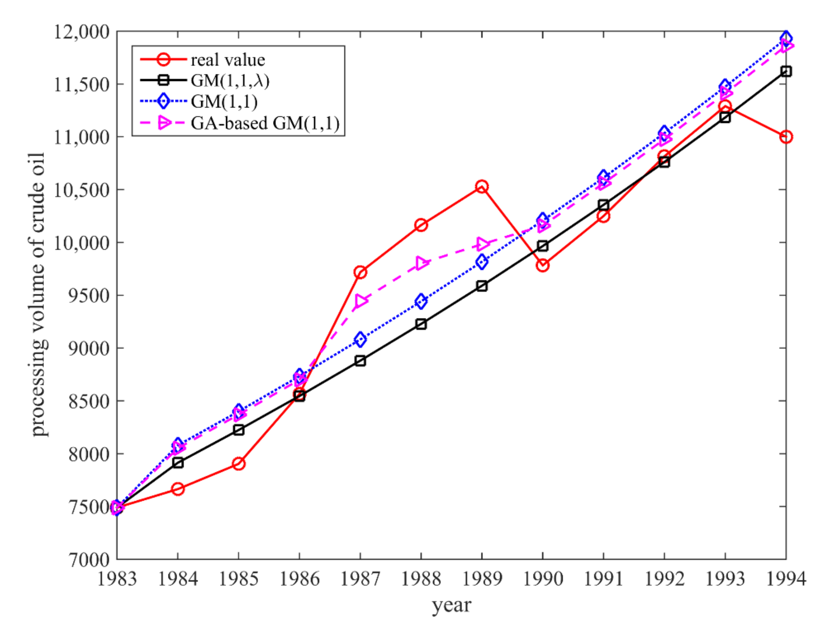
4.2. Example 2
5. Conclusions
Author Contributions
Funding
Data Availability Statement
Conflicts of Interest
References
- Deng, J. Control problems of grey system. Syst. Control. Lett. 1982, 1, 288–294. [Google Scholar]
- Liu, S.; Lin, Y. Grey Systems: Theory and Applications (Understanding Complex Systems); Springer: Heidelberg/Berlin, Germany, 2011. [Google Scholar]
- Wen, K.L. Grey Systems: Modeling and Prediction; Yang’s Scientific Press: Tucson, AZ, USA, 2004. [Google Scholar]
- Hodzic, M.; Tai, L.C. Grey predictor reference model for assisting particle swarm optimization for wind turbine control. Renew. Energy 2016, 86, 251–256. [Google Scholar] [CrossRef]
- Zhao, H.; Guo, S. An optimized grey model for annual power load forecasting. Energy 2016, 107, 272–286. [Google Scholar] [CrossRef]
- Zhou, W.; He, J.M. Generalized GM (1, 1) model and its application in forecasting of fuel production. Appl. Math. Model. 2013, 37, 6234–6243. [Google Scholar] [CrossRef]
- Shi, X.; Wang, Z.; Wang, Z. Adaptive genetic algorithm GM(1,1;λ) model and its application. Int. J. Nonlinear Sci. 2011, 11, 195–199. [Google Scholar]
- Ou, S.L. Forecasting agricultural output with an improved grey forecasting model based on the genetic algorithm. Comput. Electron. Agric. 2012, 85, 33–39. [Google Scholar] [CrossRef]
- Lee, Y.S.; Tong, L.I. Forecasting energy consumption using a grey model improved by incorporating genetic programming. Energy Convers. Manag. 2011, 52, 147–152. [Google Scholar] [CrossRef]
- Wang, Z.-X.; Hao, P. An improved grey multivariable model for predicting industrial energy consumption in China. Appl. Math. Model. 2016, 40, 5745–5758. [Google Scholar] [CrossRef]
- Hu, Y.C. Nonadditive grey prediction using functional-link net for energy demand forecasting. Sustainability 2017, 9, 1166. [Google Scholar] [CrossRef] [Green Version]
- Nan, H.T. Design a grey prediction model based on genetic algorithm for better forecasting international tourist arrivals. J. Grey Syst. 2016, 19, 7–12. [Google Scholar]
- Zhao, Z.; Wang, J.; Zhao, J.; Su, Z. Using a grey model optimized by differential evolution algorithm to forecast the per capita annual net income of rural households in China. Omega 2012, 40, 525–532. [Google Scholar] [CrossRef]
- Wang, C.H.; Hsu, L.C. Using genetic algorithms grey theory to forecast high technology industrial output. Appl. Math. Comput. 2008, 195, 256–263. [Google Scholar] [CrossRef]
- Lia, Y.; Lingb, L.; Chenb, J. Combined grey prediction fuzzy control law with application to road tunnel ventilation system. J. Appl. Res. Technol. 2015, 13, 313–320. [Google Scholar] [CrossRef]
- Yeh, M.F.; Lu, H.C. On some of the basic features of GM(1,1) mode. J. Grey Syst. 1996, 8, 19–35. [Google Scholar]
- Mead, J.L.; Renaut, R.A. Least squares problems with inequality constraints as quadratic constraints. Linear Algebra Appl. 2010, 432, 1936–1949. [Google Scholar] [CrossRef] [Green Version]
- Zulkifli, N.; Sorooshian, S.; Anvari, A. Modeling for regressing variables. J. Stat. Econom. Methods 2012, 1, 1–8. [Google Scholar]
- Seber, G.A.F.; Wild, C.J. Nonlinear Regression; John Wiley and Sons: New York, NY, USA, 1989. [Google Scholar]
- Coleman, T.F.; Li, Y. A reflective newton method for minimizing a quadratic function subject to bounds on some of the variables. SIAM J. Optim. 1996, 6, 1040–1058. [Google Scholar] [CrossRef]
- Myttenaere, A.; Golden, B.; Grand, B.; Rossi, F. Mean Absolute Percentage Error for regression models. Neurocomputing 2016, 5, 38–48. [Google Scholar] [CrossRef] [Green Version]
- DeLurgio, S.A. Forecasting Principles and Applications; Irwin/McGraw-Hill: New York, NY, USA, 1998. [Google Scholar]


| MAPE (%) | Forecasting Ability |
|---|---|
| <10 | High |
| 10–20 | Good |
| 20–50 | Reasonable |
| >50 | Inaccurate |
| Model | GM(1,1) | GA-Based GM(1,1) | Proposed GM(1,1;λ) | ||||
|---|---|---|---|---|---|---|---|
| Development coefficient a | −0.1313 | −0.1317 | −0.1154 | ||||
| Grey input b | 2,038,364.36 | 2,045,775,78 | 2,334,485.66 | ||||
| Background value λ | 0.5 | 0.47323 | 0.6667 | ||||
| Year | Real value | Fitting value | Relative error (%) | Fitting value | Relative error (%) | Fitting value | Relative error (%) |
| 2003 | 2,248,117 | 2,248,117 | 0 | 2,248,117 | 0 | 2,248,117 | 0 |
| 2004 | 2,950,342 | 2,493,504.536 | 15.48 | 2,503,172.299 | 15.16 | 2,749,456.515 | 6.80 |
| 2005 | 3,378,118 | 2,843,239.684 | 15.83 | 2,855,549.389 | 15.47 | 3,085,728.822 | 8.65 |
| 2006 | 3,519,827 | 3,242,028.150 | 7.89 | 3,257,531.379 | 7.45 | 3,463,128.918 | 1.61 |
| 2007 | 3,716,063 | 3,696,750.079 | 0.52 | 3,716,101.261 | 0.00 | 3,886,686.936 | 4.59 |
| 2008 | 3,845,187 | 4,215,250.612 | 9.62 | 4,239,225.037 | 10.25 | 4,362,048.222 | 13.44 |
| 2009 | 4,395,004 | 4,806,475.241 | 9.36 | 4,835,990.102 | 10.03 | 4,895,548.575 | 11.38 |
| 2010 | 5,567,277 | 5,480,624.135 | 1.56 | 5,516,763.102 | 0.91 | 5,494,298.694 | 1.31 |
| 2011 | 6,087,484 | 6,249,328.127 | 2.66 | 6,293,370.020 | 3.38 | 6,166,278.953 | 1.29 |
| 2012 | 7,311,470 | 7,125,849.368 | 2.54 | 7,179,301.608 | 1.81 | 6,920,445.764 | 5.34 |
| 2013 | 8,016,280 | 8,125,310.144 | 1.36 | 8,189,947.741 | 2.17 | 7,766,850.955 | 3.11 |
| 2014 | 9,910,204 | 9,264,953.766 | 6.51 | 9,342,864.761 | 5.72 | 8,716,775.741 | 12.04 |
| MAPE (%) | 6.67 | 6.58 | 6.33 | ||||
| Model | GM(1,1) | GA-Based GM(1,1) | Proposed GM(1,1;λ) | ||||
|---|---|---|---|---|---|---|---|
| Development coefficient a | −0.03897 | −0.03879 | −0.03841 | ||||
| Grey input b | 7631.41 | 7632 | 7475.61 | ||||
| Background value λ | 0.5 | 0.46 | 1.0 | ||||
| Year | Real value | Fitting value | Relative error (%) | Fitting value | Relative error (%) | Fitting value | Relative error (%) |
| 1983 | 7490 | 7490 | 0 | 7490 | 0 | 7490 | 0 |
| 1984 | 7665 | 8079.68 | 5.41 | 8052 | 5.04 | 7914.36 | 3.25 |
| 1985 | 7904 | 8400.75 | 6.28 | 8370 | 5.89 | 8224.29 | 4.05 |
| 1986 | 8565 | 8734.58 | 1.98 | 8700 | 1.57 | 8546.36 | 0.22 |
| 1987 | 9718 | 9081.67 | 6.54 | 9444 | 2.81 | 8881.05 | 8.61 |
| 1988 | 10,164 | 9442.56 | 7.09 | 9802 | 3.56 | 9228.84 | 9.20 |
| 1989 | 10,528 | 9817.78 | 6.74 | 9983 | 5.17 | 9590.25 | 8.91 |
| 1990 | 9783 | 10,207.92 | 4.34 | 10,158 | 3.83 | 9965.82 | 1.87 |
| 1991 | 10,250 | 10,613.56 | 3.54 | 10,560 | 3.02 | 10,356.09 | 1.03 |
| 1992 | 10,815 | 11,035.32 | 2.03 | 10,977 | 1.49 | 10,761.65 | 0.49 |
| MAPE (%) | 4.89 | 3.60 | 4.18 | ||||
| 1993 | 11,290 | 11,473.84 | 1.62 | 11,412 | 1.08 | 11,183.09 | 0.95 |
| 1994 | 11,000 | 11,929.78 | 8.45 | 11,946 | 8.60 | 11,621.03 | 5.65 |
| MAPE (%) | 5.04 | 4.84 | 3.30 | ||||
Publisher’s Note: MDPI stays neutral with regard to jurisdictional claims in published maps and institutional affiliations. |
© 2021 by the authors. Licensee MDPI, Basel, Switzerland. This article is an open access article distributed under the terms and conditions of the Creative Commons Attribution (CC BY) license (https://creativecommons.org/licenses/by/4.0/).
Share and Cite
Yeh, M.-F.; Chang, M.-H. GM(1,1;λ) with Constrained Linear Least Squares. Axioms 2021, 10, 278. https://doi.org/10.3390/axioms10040278
Yeh M-F, Chang M-H. GM(1,1;λ) with Constrained Linear Least Squares. Axioms. 2021; 10(4):278. https://doi.org/10.3390/axioms10040278
Chicago/Turabian StyleYeh, Ming-Feng, and Ming-Hung Chang. 2021. "GM(1,1;λ) with Constrained Linear Least Squares" Axioms 10, no. 4: 278. https://doi.org/10.3390/axioms10040278
APA StyleYeh, M.-F., & Chang, M.-H. (2021). GM(1,1;λ) with Constrained Linear Least Squares. Axioms, 10(4), 278. https://doi.org/10.3390/axioms10040278