Grey Estimator-Based Tracking Controller Applied to Swarm Robot Formation

Abstract

Mobile robots are widely used in many applications, while various types of mobile robots and their control researches have been proposed in literature. Since swarm robots have higher flexibility and capacity for teamwork, this paper presents a grey estimator-based tracking controller for formation trajectory tracking of swarm robots. First, wheel-type mobile robots are used and modeled for the controller design. Then, a grey dynamic estimator is developed to estimate the environmental disturbance and model uncertainty for linear feedback compensation. As a result, the asymptotic trajectory tracking is assured, so that the application on the swarm robot formation is achieved for a multi-agent system. The computational complexity is slightly reduced by the design. Finally, in order to verify the reliability of swarm robot formation, several types of formation are maintained by the grey estimator-based feedback linearization controller.

1. Introduction

Professor Deng published the grey system theory for data processing in the international journal System & Control Letters in 1982 [1]. From his first work, there are many applications proposed in literature, such as fields of environmental engineering, water conservancy, business management, electrical machinery, civil engineering, industry, transportation, etc. The complete grey theory is continuously developed including grey modeling [2], correlation analysis, grey control [3], grey prediction [4], grey decision-making [5,6], etc. To realize the prediction of data systems, the grey model GM (1,1) has been proposed, e.g., [7]. In detail, two steps are needed to obtain high prediction accuracy for data correction. The first is data preprocessing, which is to process the data entering the grey model, and the second step is to set the correction range and add it to GM (1,1) model. After the data preprocessing and adding correction factor into the grey data model, the accuracy of data prediction will be improved.

Currently, the grey theory is also applied on control systems, such as the speed control of servo motors [8], cyber security incidents [9,10], and road overtaking control [11]. In detail, to prevent the occurrence of network security incidents, the grey forecasts can be used to predict cyber risks based on limited dynamic data and to avoid harm [9,10]. Similarly, the grey theory realizes effective prediction of reasonable overtaking paths and data through electronic police to effectively control the safety of the road network [11]. In order to reduce the influence of external interference on the control system, a grey estimator for interference is used to compensate the interference in the feedback control loop. For example, the rod pumping system adopts the grey predictive control method, which effectively monitors the situation and performs targeted treatment in advance [12]. Additionally, the prediction performance of the grey theory [13] can be improved by combining neural network modeling. The other application on sensorless control is achieved by developing the grey estimator-based fuzzy PID [14], where the grey estimator can evaluate the torque of the motor. However, the above methods do not consider the robustness analysis in the design. This means that the grey estimator still needs to be improved.

There are many methods to achieve precise positioning, high repeatability, long-term investment for robots, such that robots can help people to do tasks which are difficult to achieve or perform by a human—such as automatic guiding, automatic storage, unmanned exploration, etc. Moreover, applying robotic systems can minimize the possible harm for people in the dangerous working environments. For the studies of robots, the autonomous mobile robot system [15] is an intelligent technology integrating navigation, sensing, electronics, image processing, and automatic control. The wheeled mobile robot (WMR) is a common autonomous mobile robot. With its non-radius of gyration and high flexibility, it is more valued than other autonomous mobile robots. For an unmanned operation and automatic navigation WMR, an important part is the ability to complete unmanned navigation technology. In detail, in a known navigation environment, the global path planning method [16], is proposed for the optimal path planning between the start point and the end point. After the path is planned, the WMR must track the reference path by designing controllers [17,18]. Furthermore, the grey theory was applied on controlling autonomous mobile robots, e.g., the authors in [19] put forward a new grey hierarchical fuzzy controller for position prediction and path tracking. However, there are still many problems to be considered in the tracking control of autonomous mobile robots on the general path tracking, e.g., unknown internal conditions or external disturbances. On the other hand, a multi-agent system is a collaborative intelligent system composed of many interactive computing entities which can solve complex tasks based on minimal or reduced data processing resources. These systems are composed of many homogeneous or heterogeneous intelligent software or hardware agents. They are agents with certain perception, communication, computing, and execution capabilities to form a system [20,21,22]. In other words, the swarm robot system can be a multi-agent system by properly designing the path tracking controller and the path profiles (i.e., several formation types). Thus, the control of swarm robots presents a challenge as to how to find a good way to achieve trajectory tracking and formation control.

In this study, the grey disturbance estimator is designed for feedback compensation. By adding the grey data prediction model, the path tracking is achieved with high robustness which is less discussed in literature. Since the grey estimator-based tracking controller assures stable path tracking, the trajectories of each robot of the swarm are achieved, such that the formation is assured for multi-agent system applications.

The remainder of this paper is organized as follows. First, we formulate the motion model of the two-wheeled mobile robot in Section 2. Next, Section 3 presents the grey estimator for the external interference to the robot, and the grey estimator-based feedback compensation is designed for robust trajectory tracking. Then, Section 4 introduces the robot multi-agent system and formation for the reference trajectory design. The simulation results are given in Section 5. Finally, some conclusions are made in Section 6.

2. Motion Model of Two-Wheeled Mobile Robot

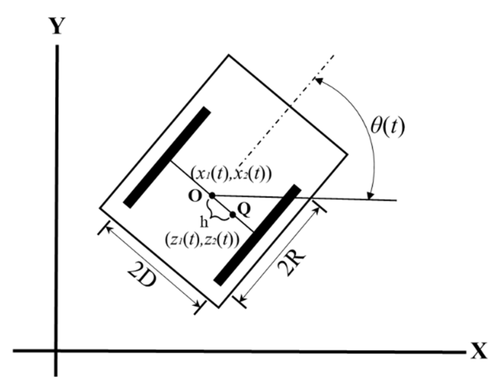
In this paper, the multi-agent system is consisted of several two-wheeled mobile robots. Here, the wheel-type autonomous mobile robot is illustrated as shown in Figure 1. The center position coordinates of the wheel-type autonomous mobile robot on the XY plane (O) can be expressed as $x_1(t)$ and $x_2(t)$. The angle between the X axis and the wheeled autonomous mobile robot on the two-dimensional plane is denoted as $x_3(t)$. The following formula is the wheel-type autonomous mobile robot model

$$\dot{x}=\mathsf{\Psi }(x(t))\overline{u}(t)$$

(1)

where $x(t)={\left[\begin{array}{ccc}{x}_1(t)& x_2(t)& x_3(t)\end{array}\right]}^T$; $\overline{u}(t)=\left[\begin{array}{l}{\overline{u}}_1(t)\\ {\overline{u}}_2(t)\end{array}\right]=\left[\begin{array}{l}\frac{1}{2}({\omega }_r+{\omega }_l)\\ \frac{1}{2}({\omega }_r-{\omega }_l)\end{array}\right]$ with the angular velocities of the right and left wheels expressed as ${\omega }_r$ and ${\omega }_l$; and

$$\mathsf{\Psi }(x(t))=\left[\begin{array}{cc}R\cos (x_3(t))& 0\\ R\sin (x_3(t))& 0\\ 0& R/D\end{array}\right]\left[\begin{array}{l}{\overline{u}}_1(t)\\ {\overline{u}}_2(t)\end{array}\right]$$

(2)

As shown in Figure 1, we add a reference point Q on the mobile robot. From the definition distance offset $h$ between the center position and the reference point Q, the following formula is the position coordinate of the reference point Q

$$z(t)=\left[\begin{array}{l}{z}_1(t)\\ z_2(t)\end{array}\right]=\left[\begin{array}{l}{x}_1(t)+h\sin (x_3(t))\\ x_2(t)-h\cos (x_3(t))\end{array}\right]$$

(3)

From (1) and (2), we can get the motion equation of Q as

$$\dot{z}(t)=\left[\begin{array}{l}{\dot{z}}_1(t)\\ {\dot{z}}_2(t)\end{array}\right]=\left[\begin{array}{l}R{z}_3(t)\cos (x_3(t))\\ R{z}_3(t)\sin (x_3(t))\end{array}\right]$$

(4)

In the above Equation (4), $z_3={\overline{u}}_1+\frac{h}{D}{\overline{u}}_2$. Here we assume that the above equation does not equal to zero, and ${\dot{z}}_3=v_1(t)$ has a virtual control input $v_1$. Next, the following equation is obtained

$$\ddot{z}(t)=\left[\begin{array}{cc}R\cos (x_3(t))& R^2{z}_3(t)\sin (x_3(t))\\ R\sin (x_3(t))& R^2{z}_3(t)\cos (x_3(t))\end{array}\right]\left[\begin{array}{l}{v}_1(t)\\ {\overline{u}}_2(t)\end{array}\right]$$

Thus, the previous formula can be expanded in the form

$$\begin{array}{cc}\dot{\overline{x}}& =\left[\begin{array}{l}{\dot{\overline{x}}}_1(t)\\ {\dot{\overline{x}}}_2(t)\\ {\dot{\overline{x}}}_3(t)\\ {\dot{\overline{x}}}_4(t)\end{array}\right]=\left[\begin{array}{l}{\dot{z}}_1(t)\\ {\dot{z}}_2(t)\\ {\ddot{z}}_1(t)\\ {\ddot{z}}_2(t)\end{array}\right]=\left[\begin{array}{cccc}0& 0& 1& 0\\ 0& 0& 0& 1\\ 0& 0& 0& 0\\ 0& 0& 0& 0\end{array}\right]\left[\begin{array}{l}{\overline{x}}_1(t)\\ {\overline{x}}_2(t)\\ {\overline{x}}_3(t)\\ {\overline{x}}_4(t)\end{array}\right]\\ & +\left[\begin{array}{cc}0& 0\\ 0& 0\\ R\cos (x_3(t))& -R^2{z}_3(t)\sin (x_3(t))\\ R\sin (x_3(t))& R^2{z}_3(t)\cos (x_3(t))\end{array}\right]\left[\begin{array}{l}{v}_1(t)\\ {\overline{u}}_2(t)\end{array}\right]\\ & \equiv A\overline{x}+B(z_3,x_3)u\hfill \end{array}$$

(5)

where $\overline{x}$ is the new defined control state vector; and $u$ is the virtual control input. Since the control input is transformed to the new coordinate, the original control target becomes a reference path tracking of the point Q for the autonomous mobile robot.

3. Grey Estimator-Based Tracking Control

There are many interference signals to mobile robots in the actual environment, most of these signals are unnecessary and disturbed for controlling autonomous mobile robots. This issue must be considered when designing path tracking control for better tracking performance. In order to solve the interference problem in the system, this study will design a grey estimator to evaluate interference and disturbance for feedback linearization compensation. Through the grey interference estimation and compensation, the grey estimator-based tracking controller will simplify the difficulty for implementing the swarm robot formation.

To this end, the dynamic model of one autonomous mobile robot of the swarm robots considering interference and disturbance is represented in the form

$$\begin{array}{cc}\dot{\overline{x}}(t)& =\left[\begin{array}{c}{\dot{\overline{x}}}_1(t)\\ {\dot{\overline{x}}}_2(t)\\ {\dot{\overline{x}}}_3(t)\\ {\dot{\overline{x}}}_4(t)\end{array}\right]=\left[\begin{array}{cccc}0& 0& 1& 0\\ 0& 0& 0& 1\\ 0& 0& 0& 0\\ 0& 0& 0& 0\end{array}\right]\left[\begin{array}{c}{\overline{x}}_1(t)\\ {\overline{x}}_2(t)\\ {\overline{x}}_3(t)\\ {\overline{x}}_4(t)\end{array}\right]\hfill \\ & +\left[\begin{array}{cc}0& 0\\ 0& 0\\ 1& 0\\ 0& 1\end{array}\right]\left[\begin{array}{c}{\tau }_1(t)+\omega (t)\\ {\tau }_2(t)+\omega (t)\end{array}\right]\hfill \\ & \equiv A\overline{x}(t)+\overline{B}(\tau (t)+\omega (t))\hfill \end{array}$$

(6)

where $\omega (t)$ is an equivalent disturbance; and the control input obtained after the coordinate conversion (5) is expressed as $\tau (t)={[{\tau }_1(t) {\tau }_2(t)]}^T$:

$$\begin{array}{l}\tau (t)=\left[\begin{array}{cc}R\cos (x_3(t))& -R^2{z}_3(t)\sin (x_3(t))\\ R\sin (x_3(t))& R^2{z}_3(t)\cos (x_3(t))\end{array}\right]\left[\begin{array}{c}{v}_1\\ {\overline{u}}_2\end{array}\right]\\ \equiv B_{s}u(t)\end{array}$$

For the application of swarm robot formation, the reference path tracking model for the robot (6) is represented by the reference state $x_R$(t) with the dynamics

$$\begin{array}{ll}{\dot{\overline{x}}}_R(t)& =\left[\begin{array}{c}{\dot{\overline{x}}}_{1R}(t)\\ {\dot{\overline{x}}}_{2R}(t)\\ {\dot{\overline{x}}}_{3R}(t)\\ {\dot{\overline{x}}}_{4R}(t)\end{array}\right]=\left[\begin{array}{cccc}0& 0& 1& 0\\ 0& 0& 0& 1\\ 0& 0& 0& 0\\ 0& 0& 0& 0\end{array}\right]\left[\begin{array}{c}{\overline{x}}_{1R}(t)\\ {\overline{x}}_{2R}(t)\\ {\overline{x}}_{3R}(t)\\ {\overline{x}}_{4R}(t)\end{array}\right]\\ & +\left[\begin{array}{cc}0& 0\\ 0& 0\\ 1& 0\\ 0& 1\end{array}\right]\left[\begin{array}{c}{\tau }_{1R}(t)\\ {\tau }_{2R}(t)\end{array}\right]\\ & \equiv A\overline{x}(t)+\overline{B}{\tau }_R(t)\end{array}$$

(7)

where ${\tau }_R(t)=\left[\begin{array}{cc}R\cos (x_{3R}(t))& -R^2{z}_{3R}(t)\sin (x_{3R}(t))\\ R\sin (x_{3R}(t))& R^2{z}_{3R}(t)\cos (x_{3R}(t))\end{array}\right]\left[\begin{array}{c}{v}_{1R}\\ u_{2R}\end{array}\right]\equiv B_s{u}_R(t)$; and the reference input $u_R(t)$ is designed for the desired swarm robot formation trajectory of corresponding mobile robot. In order to track the reference path $x_R$(t) for the autonomous mobile robot, it is necessary to design a control law to achieve the goal.

First, define a control error for the goal as $E(t)=\overline{x}(t)-x_R(t)$. The error equation is written as

$$\dot{E}(t)=AE(t)+\overline{B}(\tilde{\tau }(t)+\omega (t))$$

(8)

where $\tilde{\tau }(t)=\tau (t)-{\tau }_R(t)$ is an auxiliary control item. By using a grey feedback linearization, the auxiliary control law is designed as

$$\tilde{\tau }(t)=-\left(\widehat{\omega }(t)-KE(t)\right)$$

(9)

where K is an adjustable control gain; and $\widehat{\omega }(t)$ is an estimated value for the disturbance of the system by the grey disturbance estimator which is designed later. There is not much research related to the grey system theory for uncertain data modeling. In this study, the grey data model of the robot system is established. To get the grey interference estimator, the control law is rewritten in the form

$$u=B_S^{-1}({\tau }_R+KE-\widehat{\omega })$$

(10)

In addition, the following equation is obtained by substituting (9) into (8) as

$$\dot{E}(t)=(A+\overline{B}K)E(t)+\overline{B}(\omega (t)-\widehat{\omega }(t))$$

(11)

Here, it is necessary to adjust the feedback gain value K such that the closed-loop control system is asymptotically stable. In order to ensure the robustness of the control performance, the last term of the Equation (11) must be approached to zero. Besides, the grey interference estimator is designed to avoid external interference to the closed-loop system.

Then, to design the grey interference estimator, the data collection procedure is expressed for the state $\overline{x}(t)$ as

$$x_{new}^{(0)}(k)={\overline{x}}^{(0)}(t)$$

(12)

The sequence of the data obtained after discretization of ${\overline{x}}^{(0)}(t)$ is $x_{new}^{(0)}(k)$, and the result can be obtained using the formula

$$X_{new}^{(0)}=[x^{(0)}(k),x^{(0)}(k-1),x^{(0)}(k-2),x^{(0)}(k-3)]$$

Here the number of iterations is represented by k, and the total number of data is set to n. The grey model is defined after the accumulation sequence as

$${\overline{x}}_{new}^{(1)}(k)={\displaystyle \sum _{g=1}^k{\overline{x}}_{new}^{(0)}(g)}, k=1, 2,\dots , n$$

(13)

The superscript “(0)” in the above formula represents the original sequence, and the superscript “(1)” represents the accumulation and arrangement in order. The first-order ordinary differential equation of the grey model GM (1,1) is expressed by the differentiation

$$\frac{d{\overline{x}}_{new}^{(1)}}{dt}+a{\overline{x}}_{new}^{(1)}=b$$

(14)

where both a and b are grey model parameters; and a and b are the development factor and the weighting factor, respectively. The term $d{\overline{x}}_{}^{(1)}$/$dt$ is approximated by the form

$$\frac{d{\overline{x}}_{}^{(1)}}{dt}={\overline{x}}_{new}^{(1)}(k+1)-{\overline{x}}_{new}^{(1)}(k)={\overline{x}}_{new}^{(0)}(k+1)$$

(15)

Letting ${\overline{x}}_{new}^{(1)}$ of (14) replaced by the average of ${\overline{x}}_{new}^{(1)}(k+1)$ and ${\overline{x}}_{new}^{(1)}(k)$ and substituting (15) into (14), the following equation is obtained as

$${\overline{x}}_{new}^{(0)}(k+1)=a\left\{-\frac{1}{2}\left[{\overline{x}}_{new}^{(1)}(k+1)+{\overline{x}}_{new}^{(1)}(k)\right]\right\}+b$$

(16)

To obtain the grey model parameters of the GM(1,1) model, the linear regression method is used and leads to

$${[a b]}^T=(Y_G^T{Y}_G{}^{-1})Y_G^T{Y}_N$$

(17)

where

$$Y_N={\left[{\overline{x}}_{new}^{(0)}(1) {\overline{x}}_{new}^{(0)}\left(2\right) \cdots {\overline{x}}_{new}^{(0)}\left(n\right)\right]}^{\mathrm{T}},{\mathrm{Y}}_{\mathrm{G}}=\left(\begin{array}{cc}-0.5*({\overline{x}}_{new}^{(1)}\left(0\right)+{\overline{x}}_{new}^{(1)}\left(1\right)) \hfill & \hfill 1\\ -0.5*({\overline{x}}_{new}^{(1)}\left(1\right)+{\overline{x}}_{new}^{(1)}\left(2\right)) 1\hfill & \hfill 1\\ ⋮& \hfill ⋮\\ -0.5*({\overline{x}}_{new}^{(1)}(n-1)+{\overline{x}}_{new}^{(1)}(n\left)\right) 1\hfill & \hfill 1\end{array}\right)$$

(18)

Based on the grey model parameters (17), the first-order differential Equation (14) is solved as

$${\widehat{\overline{x}}}^{(1)}(k)=\frac{b}{a}+\left[{\overline{x}}^{(1)}(1)-\frac{b}{a}\right]e^{-ak}$$

(19)

Then, the estimated original state sequence is calculated by the inverse accumulation as

$${\widehat{\overline{x}}}^{(0)}(k+1)=-\left({\widehat{\overline{x}}}^{(1)}(k)-{\widehat{\overline{x}}}^{(1)}(k+1)\right)=\left[e^{-a}-1\right]\left[{\overline{x}}^{(0)}-\frac{b}{a}\right]e^{-ak}$$

(20)

By substitute (15) and (20) into (6) and sorting it out, we can obtain the grey inference estimator

$$\widehat{\omega }(k)=B_s^{-1}\left[0{ \mathrm{I}}_2\right]\times \left(-A{\widehat{\overline{x}}}^{(0)}(k)-\overline{B}\tau (k)+{\widehat{\overline{x}}}^{(0)}(k+1)-{\widehat{\overline{x}}}^{(0)}(k)\right)$$

(21)

By applying the above estimator, the error system is further simplified as

$$\dot{E}(t)=(A+\overline{B}K)E(t)+\overline{B}{e}_s$$

(22)

where $e_S$ is the estimation error of $\omega (t)-\widehat{\omega }(t)$. Here the gain value K will be designed arbitrarily because the above equation is said to be very basic in a linear system. We can use the eigenvalue setting method or the linear matrix inequality (LMI) method [23,24] to solve the control gain K.

To design the controller gain for system stability, we choose the Lyapunov function $V=E^{T}PE$ with the positive definite matrix P and take its differentiation as

$$\begin{array}{cc}\dot{V}& =E^T\left[\left(A^T+K^T{\overline{B}}^T\right)P+P(A+\overline{B}K)\right]E+E^{T}P\overline{B}{e}_s+e_s^T{\overline{B}}^{T}PE\hfill \\ & \le E^T\left[\left(A^T+K^T{\overline{B}}^T\right)P+P(A+\overline{B}K)\right]E+{\rho }^2{E}^{T}P\overline{B}{\overline{B}}^{T}PE+\frac{1}{{\rho }^2}{e}_s^T{e}_s\hfill \end{array}$$

(23)

To let $\dot{V}\le 0$, we obtain the stability condition

$$A^{T}P+K^T{\overline{B}}^{T}P+PA+P\overline{B}K+{\rho }^{2}P\overline{B}{\overline{B}}^{T}P+PQP<0$$

(24)

where $\rho >0$ is an error attenuation parameter; and Q is a choosing positive definite matrix. If the condition (24) is satisfied, then the system achieves

$$\dot{V}\le -E^{T}PQPE+\frac{1}{{\rho }^2}{e}_s^T{e}_s$$

As a result, the stability can be assured. By integrating both sides of the above inequality, we further obtain the robustness

$${\displaystyle {\int }_0^{t_f}{E}^T\left(t\right)}PQPE\left(t\right)dt\le E_{}^T\left(0\right)PE\left(0\right)+\frac{1}{{\rho }^2}{\displaystyle {\int }_0^{t_f}{\Vert e_s\left(t\right)\Vert }^{2}dt}$$

(25)

This means that the effect of the inference estimation error is attenuated the $1/\rho$ level. In addition, by premultiplying and postmultiplying above inequality (24) by $P^{-1}$, we reformulate the condition below

$$P^{-1}{A}^T+P^{-1}{K}^T{\overline{B}}^T+A{P}^{-1}+\overline{B}K{P}^{-1}+{\rho }^2\overline{B}{\overline{B}}^T+Q<0$$

Let M = KX and X = $P^{-1}$, and arrange the above inequality as in an LMI form

$$X{A}^T+M^T{\overline{B}}^T+AX+\overline{B}M+{\rho }^2\overline{B}{\overline{B}}^T+Q<0$$

(26)

The solution of the above LMI can be found by using the LMI toolbox of MATLAB software. Therefore, the following theorem is made below.

Theorem 1.

Considering the formation reference path of the swarm robot system (7) for the mobile robot (1) with the transformation (3) and applying the control law (10) with the grey GM (1,1) inference estimator (21), if there exist a positive definite matrix X and a control gain K satisfying the LMI (26), then the closed-loop error system assures the$H^{\infty }$tracking robustness performance (25). Moreover, when the grey inference estimation error$e_s$converges to zero, the trajectory tracking achieves the asymptotic stability.

Remark 1.

Being different to other grey estimator studies, this paper assures the robustness of the closed-loop control system even if there exist grey estimator errors. The control performance can be tuned by the LMI technique. Moreover, the grey inference compensation can be easily implemented without more measurement of the mobile robot.

Remark 2.

Based on the above design, the formation reference path for one mobile robot of the swarm robot system can be tracked in an asymptotic manner. Thus, the swarm formation can be achieved. Moreover, the formation control is performed in an individual manner, where we only need the coordination for the formation trajectories.

4. Robot Multi-Agent System and Formation

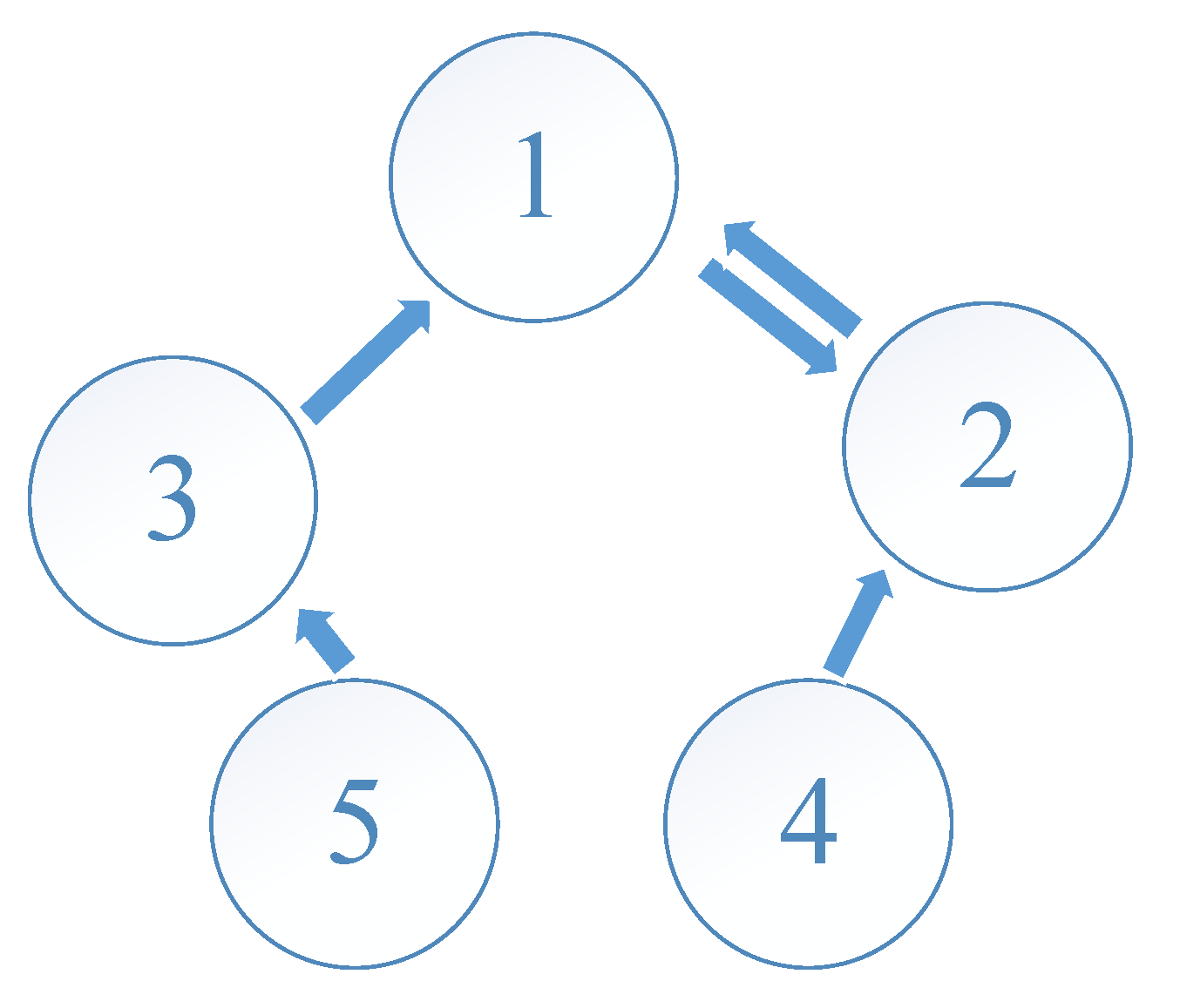
Next, the formation design is introduced for the coordination for the swarm robot system. As we know, multi-agent systems have different organizational structures depending on the interaction. Here, we will use the graphical theory to represent how messages are sent between multiple robots. Consider the directed graph shown in Figure 2, where the circle represents an agent node which is one mobile robot; the arrow direction is the direction of the massage transmission. If there are two arrows between the two agents, they can communicate in both directions. Only one arrow represents that the two nodes can only pass messages in one way.

For this agent link as shown in Figure 2, the architecture is usually described as degree matrix, Laplacian matrix, and adjacency matrix. In this study, the adjacency matrix is used and expressed as

$$\underset{\_}{A}=\left[\begin{array}{cccc}{a}_{11}& a_{12}& \cdots & a_{1m}\\ a_{21}& a_{22}& \cdots & a_{2m}\\ ⋮& ⋮& \ddots & ⋮\\ a_{m1}& a_{m2}& \cdots & a_{mm}\end{array}\right]\in R^{m\times m}$$

(27)

where $a_{ij}$ = 1, for (ν_j, ν_i)$\in \epsilon$; $a_{ij}$ = 0, for (ν_j, ν_i)$\notin \epsilon$; $a_{ii}$ = 0; ν_j and ν_i represent the j-th and i-th agents, respectively; $\epsilon$ is ν_j to ν_i connection set; m is the total number of agents. The degree matrix can be written as D = diag{d₁, d₂,…, d_m} $\in$ $R^{m\times m}$, where i = 1, 2,…, m. Then the Laplacian matrix of the graph is written as

$$L=D-\underset{\_}{A}=\left[\begin{array}{cccc}{d}_1& -a_{12}& \cdots & -a_{1m}\\ -a_{21}& d_2& \cdots & -a_{2m}\\ ⋮& ⋮& \ddots & ⋮\\ -a_{m1}& -a_{m2}& \cdots & d_m\end{array}\right]\in R^{m\times m}$$

(28)

Considering the leader-follower architecture of the multi-agent system, the (m + 1)-th robot is called a lead agent, and the other robots are called the follower agents. The lead agent can only send messages to follower agents in one way—i.e., which cannot receive messages from follower agents. This multi-agent system will amplify Laplacian’s description of its communication architecture as

$$L=\left[\begin{array}{ccccc}{\overline{d}}_1& -a_{12}& \cdots & -a_{1m}& -a_{1(m+1)}\\ -a_{21}& {\overline{d}}_2& \cdots & -a_{2m}& -a_{2(m+1)}\\ ⋮& ⋮& \ddots & ⋮& ⋮\\ -a_{m1}& -a_{m2}& \cdots & {\overline{d}}_m& -a_{m(m+1)}\\ 0& 0& \cdots & 0& 0\end{array}\right]=\left[\begin{array}{ccc}\overline{L}& |& -\overline{J}\\ ---& +& --\\ 0& |& 0\end{array}\right]$$

(29)

where ${\overline{d}}_i={\displaystyle {\sum }_{j=1}^{m+1}{a}_{ij}}$; $\overline{J}={[\begin{array}{cccc}{a}_{1(m+1)}& a_{2(m+1)}& \cdots & a_{m(m+1)}\end{array}]}^T$ is the link parameter from leader to followers, at least one of $a_{i(m+1)}$ is not zero. It is worth noting that $\overline{L}$ is a reversible matrix and has a positive real number eigenvalue.

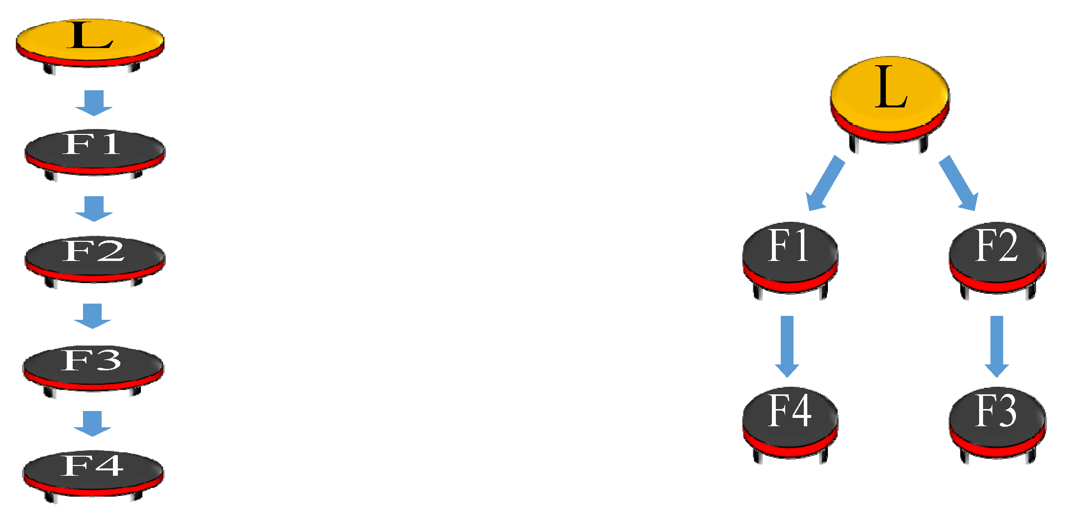
Since the above description matrix affects the design of the collaborative controller, different application forms are discussed. It is worth noting that the leadership agent can also be a virtual-leader agent, which allows the agent to make the agent system more flexibly by appropriately arrange the virtual-leader agent and make followers pursue the corresponding position to the virtual leader. As shown in Figure 3, the virtual leader (orange agent) leads the robot group. After the swarm robots pass through a narrow area by a column formation, the robot group can change to a rectangular formation. For the column formation, the virtual leader sends signals to the F1 follower, and then followers F2, F3, and F4 send signals in turn. On the other hand, for the rectangular formation, the virtual leader sends signals to F1 and F2 followers at the same time. Then F1 and F2 transmit signals to F4 and F3, respectively. The formation is maintained by the connection of these messages. While the Laplacian matrix L and $\overline{L}$ of the column formation (left of Figure 3) and the rectangular formation (right of Figure 3) are given below (30) and (31), respectively.

$$L=\left[\begin{array}{ccccc}1& 0& 0& 0& -1\\ -1& 1& 0& 0& 0\\ 0& -1& 1& 0& 0\\ 0& 0& -1& 1& 0\\ 0& 0& 0& 0& 0\end{array}\right], \overline{L}=\left[\begin{array}{cccc}1& 0& 0& 0\\ -1& 1& 0& 0\\ 0& -1& 1& 0\\ 0& 0& -1& 1\end{array}\right]$$

(30)

$$L=\left[\begin{array}{ccccc}1& 0& 0& 0& -1\\ 0& 1& 0& 0& -1\\ 0& -1& 1& 0& 0\\ -1& 0& 0& 1& 0\\ 0& 0& 0& 0& 0\end{array}\right], \overline{L}=\left[\begin{array}{cccc}1& 0& 0& 0\\ 0& 1& 0& 0\\ 0& -1& 1& 0\\ -1& 0& 0& 1\end{array}\right]$$

(31)

Based on the above connection, the positions of follower robots are designed according to relative neighbor robots. For example, considering a line formation, the position of the $\lambda -\mathrm{th}$ robot is set to

$$\begin{array}{l}{x}_{\lambda +1}=x_{\lambda }+\ell \cos {\theta }_{\lambda }\\ y_{\lambda +1}=y_{\lambda }+\ell \sin {\theta }_{\lambda }\end{array}$$

(32)

where $\left(x_{\lambda },y_{\lambda }\right)$ is the position coordinate of the $\lambda -\mathrm{th}$ robot; and ${\theta }_{\lambda }$ is the formation angle for the $(\lambda +1)-\mathrm{th}$ robot relative to the $\lambda -\mathrm{th}$ robot; and $\ell$ is the distance between the neighbor two robots. In Figure 4, the column formation has the same formation angle ${\theta }_{\lambda }=-{90}^{\circ }$. On the other hand, the row formation of the swarm in Figure 4 has the same formation angle ${\theta }_{\lambda }=0^{\circ }$. If all mobile robots can keep the relative position, the moving trajectory of the whole swarm robots can be set by designing the trajectory of the virtual leader—i.e., designing the trajectory of $\left(x_0,y_0\right)$. As a result, the motion of the formation of the swarm robots is able to be given from the task by only adjusting the reference model (7) for the virtual leader.

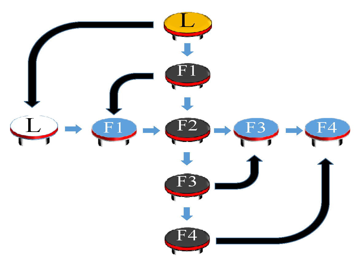
For different environments or tasks, the formation change is still achieved via the grey estimator tracking controller. The change of the design formation has three rules: (1) the moving speed of the whole formation is zero; (2) the paths of robots do not conflict; and (3) the distance required for movement is reduced as short as possible. For example, when a column formation needs to be changed to a row formation, the moving speed of the whole formation is kept at zero. The follower robots move to the fixed corresponding positions (i.e., ${\dot{\overline{x}}}_R=0$) by using the grey estimator-based tracking controller. Then, the formation transformation is completed as shown in Figure 5.

5. Simulation Results

To verify the validity of swarm robot formation control, several simulation cases are performed. In the simulation, it is assumed here that the radius R of all wheels of the autonomous mobile robot and the wheelbase h between the wheels are 0.02 m and 0.035 m, respectively. le robot and the wheelbase (h) between the wheels are 0.02 m and 0.035 m, respectively. The equivalent disturbance $\omega (t)$ is assumed as $0.001+0.001*\left(\mathrm{rand}-0.5\right)$, $rand\in \left[0,1\right]$. The controller gain K is obtained by solving the LMI (26) with the control parameters $\rho =1.1$ and Q = $\mathrm{diag}\left\{2,2,2,2\right\}$ as

$$K=\left[\begin{array}{cccc}\hfill 11.0607\hfill & \hfill 0 \hfill & \hfill -8.5611\hfill & \hfill 0\hfill \\ \hfill 0 \hfill & \hfill -11.0607\hfill & \hfill 0 \hfill & \hfill -8.5611\hfill \end{array}\right]$$

5.1. Simulation Case 1

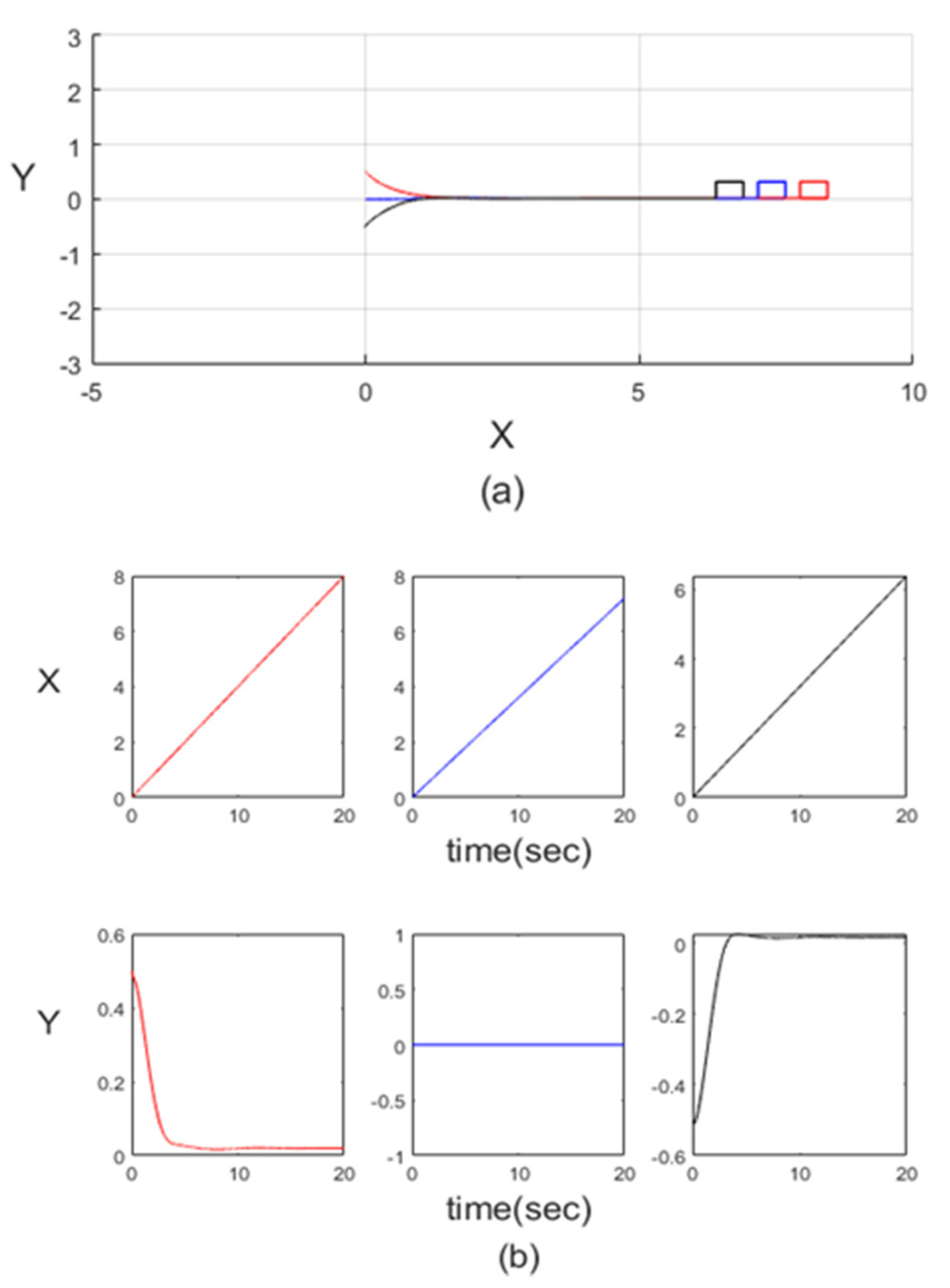
The starting points of robot 1 (red), robot 2 (blue), and robot 3 (black) are respectively set to

$$\begin{gathered} (x_{11},x_{21},x_{31})=(0, 0.5, 0.1) \\ (x_{12},x_{22},x_{32})=(0, 0, 0.1) \\ (x_{13},x_{23},x_{33})=(0,-0.5, 0.1) \end{gathered}$$

The goal is to drive the swarm robots to a column formation. To this end, the reference model (7) is used for follower robots with the position relation (32), $\lambda =1$, and ${\theta }_{\lambda }=0^{\circ }$. The motion of the whole formation is set with the reference control input $u_R={[20 0]}^T$. After applying the grey estimator-based tracking controller, the simulation result is obtained as shown in Figure 6. The swarm robots are formatted in a moving row formation.

5.2. Simulation Case 2

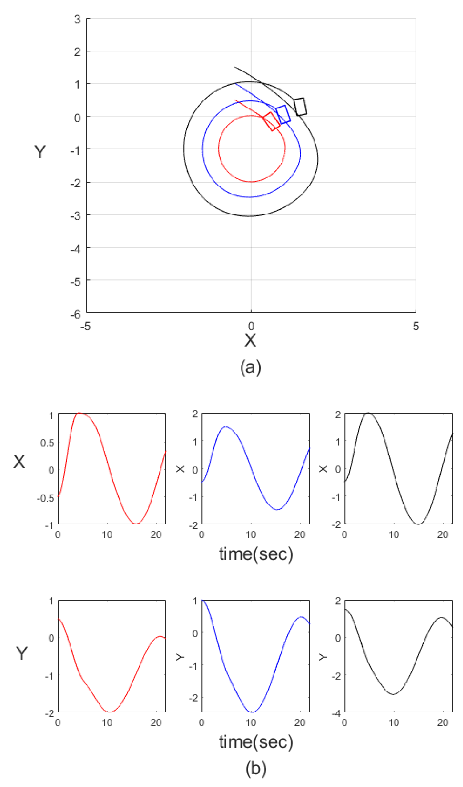
In this case, we consider a circle motion of the row formation. The reference model (7) is used for follower robots with the position relation (32) of the row formation, i.e., $\lambda =0.5$, and ${\theta }_{\lambda }=0^{\circ }$. The motion of the whole formation is set to a circle motion defined by the reference model with the control input $u={[15 -15]}^T$. Here, the starting points of robot 1 (red), robot 2 (blue), and robot 3 (black) are respectively

$$\begin{gathered} (x_{11},x_{21},x_{31})=(-0.5, 0.5, 0.1) \\ (x_{12},x_{22},x_{32})=(-0.5, 1, 0.1) \\ (x_{13},x_{23},x_{33})=(-0.5, 1.5, 0.1) \end{gathered}$$

After applying the grey estimator-based tracking controller, the simulation result is obtained as shown in Figure 7. As a result, the goal is achieved, where the swarm robots keep the row formation and take the circle motion.

Remark 3.

From the simulation verification, the swarm robot system can be easily implemented. The practical tests in a real-world environment can be realized by the proposed multi-agent structure. Each mobile robot is an agent of the formation task, while the motion trajectory can be tracked by the proposed grey estimator-based controller in a distributed manner. This means that the practical implementation will be easily achieved after the connection of the multi-agent system.

6. Conclusions

Swarm robots can do work that may not be accomplished by a single robot due to capacity limitations. In order to control swarm robots without collisions with each other, swarm robots are driven in a fixed formation which is achieved by using the proposed grey estimator-based tracking controller. By applying the grey estimator-based tracking controller, the robot reference trajectories of the desired formation can be easily designed. The asymptotic trajectory tracking is assured based on the grey estimation and LMI gain solution. Since each robot is driven to the pre-set trajectory, the formation control is achieved in an asymptotic manner. Moreover, due to the design of the virtual leader, the formation control of each robot is performed without requiring other information from other robots—i.e., the swarm robots are control in a distributed manner. Finally, the simulation has verified that the swarm robots can maintain the formation when doing different formation motion. In the future, practical tests of swarm robots in the real-world environment will be done as the research continues.

References

1. Shi, Y.; Zhu, Y. The Evaluation Model of Traditional Media Transformation Competency Based on the Grey System Theory. In Proceedings of the 2020 IEEE International Conference on Systems, Man, and Cybernetics (SMC), Toronto, ON, Canada, 11–14 October 2020; pp. 2882–2886. [Google Scholar]
2. Kang, Y.; Mao, S.; Zhang, Y.; Zhu, H. Fractional derivative multivariable grey model for nonstationary sequence and its application. J. Syst. Eng. Electron. 2020, 31, 1009–1018. [Google Scholar]
3. He, S.; Wang, M. Grey Prediction PI Control of Direct Drive Permanent Magnet Synchronous Wind Turbine. In Proceedings of the 2020 IEEE 4th Conference on Energy Internet and Energy System Integration (EI2), Wuhan, China, 30 October–1 November 2020; pp. 2032–2035. [Google Scholar]
4. Run, L.; Min, L.X.; Lu, Z.X. Research and Comparison of ARIMA and Grey Prediction Models for Subway Traffic Forecasting. In Proceedings of the 2020 International Conference on Intelligent Computing, Automation and Systems (ICICAS), Chongqing, China, 11–13 December 2020; pp. 63–67. [Google Scholar]
5. Xiao, Q.; Shan, M.; Gao, M.; Xiao, X. Grey information coverage interaction relational decision making and its application. J. Syst. Eng. Electron. 2020, 31, 359–369. [Google Scholar] [CrossRef]
6. Tian, G.; Hao, N.; Zhou, M.; Pedrycz, W.; Zhang, C.; Ma, F.; Li, Z. Fuzzy Grey Choquet Integral for Evaluation of Multicriteria Decision Making Problems with Interactive and Qualitative Indices. IEEE Trans. Syst. Man Cybern. Syst. 2021, 51, 1855–1868. [Google Scholar] [CrossRef]
7. Xiao, L.; Wang, H.; Duan, M. The Optimization of Grey Model GM (1,1) Based on Posterior Error. In Proceedings of the 2020 5th International Conference on Control, Robotics and Cybernetics (CRC), Wuhan, China, 16–18 October 2020; pp. 87–91. [Google Scholar]
8. Gao, F.; Wang, F.; Zhang, M.; Wu, Y. Study on Multi-Objective Intelligent Speed Controller Model of Automatic Train Operation for High Speed Train Based on Grey System Theory and Genetic Algorithm. In Proceedings of the 2018 11th International Symposium on Computational Intelligence and Design (ISCID), Hangzhou, China, 8–9 December 2018; pp. 189–194. [Google Scholar]
9. Gong, J. Network Information Security Pipeline Based on Grey Relational Cluster and Neural Networks. In Proceedings of the 2021 5th International Conference on Computing Methodologies and Communication (ICCMC), Erode, India, 8–10 April 2021; pp. 971–975. [Google Scholar]
10. Yao, J.; Wu, P.; Wang, Y.; Wang, Z.; Tang, Y. Research on Power Wireless Network Quality Evaluation Method Based on Multi-dimensional Index. In Proceedings of the 2020 IEEE International Conference on Information Technology, Big Data and Artificial Intelligence (ICIBA), Chongqing, China, 6–8 November 2020; pp. 376–381. [Google Scholar]
11. Zhang, Y.; Wu, Z.; Huang, M.; Wu, Z.; Wang, H. Application of Grey System Model in Overtaking with High Benefit. In Proceedings of the 2020 11th International Conference on Prognostics and System Health Management (PHM-2020 Jinan), Jinan, China, 23–25 October 2020; pp. 499–502. [Google Scholar]
12. Song, H.; Gao, W.; Ren, T. Research on Condition Prediction of Rod Pumping System Based on Grey Prediction Model. In Proceedings of the 2020 12th International Conference on Measuring Technology and Mechatronics Automation (ICMTMA), Phuket, Thailand, 28–29 February 2020; pp. 760–762. [Google Scholar]
13. Li, C.; Kang, Q.; Song, Y.; Wu, J. Analysis and Prediction of China’s Tourism Impact Factors Based on Grey Relational Entropy -BP Neural Network Model. In Proceedings of the 2020 International Conference on Big Data & Artificial Intelligence & Software Engineering (ICBASE), Bangkok, Thailand, 30 October–1 November 2020; pp. 250–253. [Google Scholar]
14. Liem, D.T.; Truong, D.Q.; Ahn, K. A torque estimator using online tuning grey fuzzy PID for applications to torque-sensorless control of DC motors. Mechatronics 2015, 26, 45–63. [Google Scholar] [CrossRef]
15. Tarao, S.; Fujiwara, Y.; Tsuda, N.; Takata, S. Development of Autonomous Mobile Robot Platform Equipped with a Drive Unit Consisting of Low-End In-Wheel Motors. In Proceedings of the 2020 5th International Conference on Control and Robotics Engineering (ICCRE), Osaka, Japan, 24–26 April 2020; pp. 42–47. [Google Scholar]
16. Jiang, C.; Sun, S.; Liu, J.; Fang, Z. Global path planning of mobile robot based on improved JPS+ algorithm. In Proceedings of the 2020 Chinese Automation Congress (CAC), Shanghai, China, 6–8 November 2020; pp. 2387–2392. [Google Scholar]
17. Bai, G.; Meng, Y.; Gu, Q.; Gan, X.; Liu, L. MPC-Based Path Tracking of Mobile Robots in the Non-Global Coordinate System. In Proceedings of the 2019 Chinese Control and Decision Conference (CCDC), Nanchang, China, 3–5 June 2019; pp. 6071–6075. [Google Scholar]
18. Jia, Q.; Chang, C.; Zhang, L.; Zhang, S. Path Tracking Control of Omnidirectional Mobile Robot Based on Bidirectional Visual Navigation. In Proceedings of the 2019 Chinese Control and Decision Conference (CCDC), Nanchang, China, 3–5 June 2019; pp. 5579–5584. [Google Scholar]
19. Moran, A.; Nagai, M. Autonomous Driving of Truck-Trailer Mobile Robots with Linear-Fuzzy Control for Trajectory Following. In Proceedings of the 2020 IEEE International Conference on Fuzzy Systems (FUZZ-IEEE), Glasgow, UK, 19–24 July 2020; pp. 1–8. [Google Scholar]
20. Feng, Y.; Lu, G.; Bai, W.; Zhao, J.; Bai, Y.; Xu, T. Rapid Coverage Control with Multi-agent Systems Based on K-Means Algorithm. In Proceedings of the 2020 7th International Conference on Information, Cybernetics, and Computational Social Systems (ICCSS), Guangzhou, China, 13–15 November 2020; pp. 870–874. [Google Scholar]
21. Victor, A.; Viorica, S.; Silvia, M.; Dimitrie, B.; Dmitri, C.; Ana, N.; Sergiu, D. Multi-agent cognitive system for optimal solution search. In Proceedings of the 2018 International Conference on Development and Application Systems (DAS), Suceava, Romania, 24–26 May 2018; pp. 53–56. [Google Scholar]
22. Stefanova-Stoyanova, V.; Stankov, I. Multi-agent systems (MAS) in the area of IoT and using a model with Distributed Shared Memory system (DSM). In Proceedings of the 2020 International Scientific Conference Electronics (ET), Sozopol, Bulgaria, 16–18 September 2020; pp. 1–4. [Google Scholar]
23. Faisal, M.; Singh Lather, J. State Derivative Feedback Control for Boost Converter via Linear Matrix Inequalities. In Proceedings of the 2020 First IEEE International Conference on Measurement, Instrumentation, Control and Automation (ICMICA), Kurukshetra, India, 24–26 June 2020; pp. 1–4. [Google Scholar]
24. Rapoport, L.; Tormagov, T. On the Solvability of Linear Matrix Inequalities under Quadratic Constraints. In Proceedings of the 2020 15th International Conference on Stability and Oscillations of Nonlinear Control Systems (Pyatnitskiy’s Conference) (STAB), Moscow, Russia, 3–5 June 2020; pp. 1–3. [Google Scholar]
Figure 1. Autonomous mobile robot model.
Axioms 10 00298 g001
Figure 2. Directed graph of multi agent system.
Axioms 10 00298 g002
Figure 3. Column formation (left) and rectangular formation (right).
Axioms 10 00298 g003
Figure 4. Column (left) and row (right) formation.
Axioms 10 00298 g004
Figure 5. Column formation changes to row formation.
Axioms 10 00298 g005
Figure 6. (a) Formation result of swarm robots; (b) position responses of the robots.
Axioms 10 00298 g006
Figure 7. (a) Formation control of the swarm robots; (b) position response in the XY axis of the three robots.
Axioms 10 00298 g007
Publisher’s Note: MDPI stays neutral with regard to jurisdictional claims in published maps and institutional affiliations.