Article

Turbulence Models for Single Phase Flow Simulation of Cyclonic Flotation Columns

1
School of Chemical Engineering and Technology, China University of Mining and Technology, Xuzhou 221116, China
2
School of Power Engineering, China University of Mining and Technology, Xuzhou 221116, China
3
Chinese National Engineering Research Center of Coal Preparation and Purification, Xuzhou 221116, China
*
Authors to whom correspondence should be addressed.
Minerals 2019, 9(8), 464; https://doi.org/10.3390/min9080464
Submission received: 10 June 2019 / Revised: 21 July 2019 / Accepted: 25 July 2019 / Published: 30 July 2019

Abstract

:
Cyclonic fields are important for cyclonic static microbubble flotation columns (FCSMCs), one of the most important developments in column flotation technology, particularly for separation of fine particles, where the internal flow field has enormous influence on flotation performance. PIV (particle image velocimetry) and CFD (computational fluid dynamics) are the most effective methods to study flow fields. However, data is insufficient for FCSMC flow fields and similar cyclonic equipment, with turbulence model simulations producing different views to measured data. This paper employs an endoscope and PIV to measure axial and cross sections for single-phase swirling flow fields in FCSMCs. We then compare various turbulence model simulations (Reynolds stress model (RSM), standard k-ε, realizable k-ε, and RNG (renormalization group) k-ε) to the measured data. The RSM (Reynolds stress model) predicts cyclonic flow field best in flotation columns with 16.22% average relative velocity deviation. Although the realizable k-ε model has less than 30% relative deviation in radial and tangential directions, axial deviations reach 78.11%. Standard k-ε and RNG k-ε models exhibited approximately 40% and 30% radial and tangential deviation, respectively, and cannot be used even for trend predictions for axial velocity. k-ε models are based on isotropic assumptions with semi-empirical formulas summarized from experiments, whereas RSM fundamentally considers laminar flow and Reynolds stress, and hence is more suitable for anisotropic performance. This study will contribute to flotation column and other cyclonic flow field equipment research.

1. Introduction

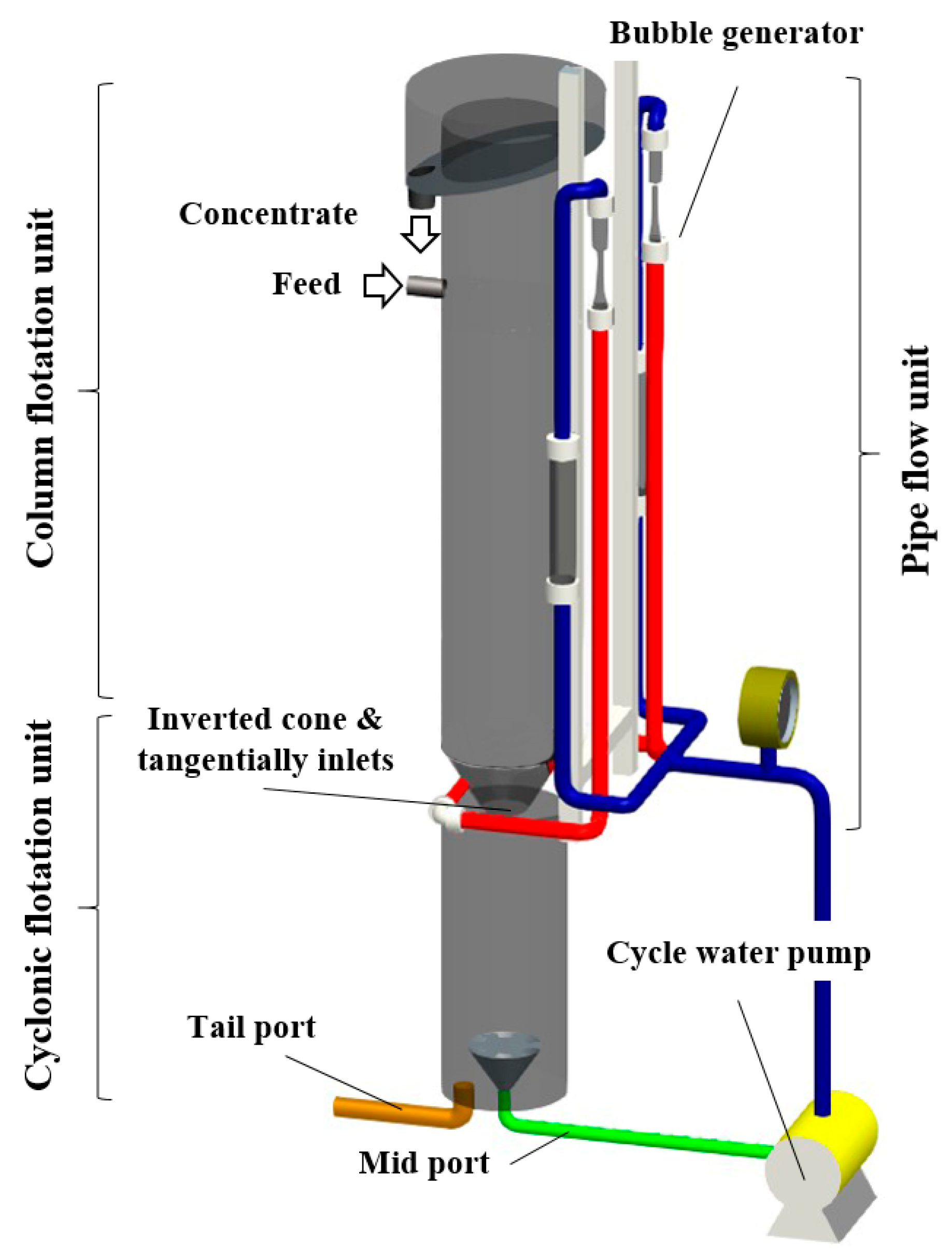
Cyclonic structures are employed in cyclonic static microbubble flotation columns (FCSMCs), which have sprung up since it was patented in 1999 [1] and been successfully applied to refining stages, to facilitate centrifugal separation [2], bubble dispersion [3], and the reduction of sorting granularity [4]. Figure 1 shows a typical FCSMC structure, incorporating an inverted cone in its middle part. Air is introduced and crushed into microbubbles by bubble generators in the pipe flow. The mixture of slurry and bubbles enters the flotation column from two symmetrical inlets on the swirl inverted cone, forming a swirl flow field. Hydrophobic mineral particles attach to the bubbles and are carried up to be concentrated. Under the centrifugal force in the swirling flow field, the high-density and coarse particles move outward and are discharged from the tail port. The remaining minerals enter the mid port and are separated again in the following pipe flow unit. This complex process involve lift, drag, and other interaction since gas and particles move in liquid. Under liquid forces and interface forces, collisions, adhesions, and detachments between particles and bubbles happen, as shown in Figure 2. Generally, this process happened in a turbulence flow environment [5] and are affected by the turbulent flow field. Therefore, the turbulence in cyclonic flow fields is an important research topic for this type of flotation column and other similar equipment.
Fine mineral particles and water are thoroughly mixed in a stirred tank to form a homogeneous slurry, and then introduced into the flotation column. Flotation feed particles are generally <0.074 mm in diameter, and flow well in the slurry. This work will provide an important reference for the study of multiphase flow in a flotation column and will have a positive impact on the industrial application of flotation columns.
Flow fields have been studied for many years with continuous developments in experimental fluid dynamics (EFD) and computational fluid dynamics (CFD). Particle image velocimetry (PIV) is an advanced EFD-based velocity measurement method developed in the late 1970s. PIV can record velocity distribution information for a large number of spatial points in the same transient state, providing flow field structure and characteristics [6].
Although PIV has been widely used for cyclonic flow field measurement, data remains inadequate to fully reflect detailed flow features. For example, Marins et al. [7] used PIV to measure axial and tangential velocity of a hydrocyclone without an air core to obtain the radial velocity. Cui et al. [8] used PIV to measure axial and radial velocity in the axial section of a hydrocyclone with an air core, but cross-section measurement was not possible due to overflow. Tangential velocity is particularly difficult to measure for flotation columns since the column top is open and the swirling flow interferes with the light path. Yan et al. [9] and Wang et al. [10] used PIV to measure single-phase cyclonic flow fields for flotation columns, but only obtained axial velocity by measuring one quasi axial section of the flotation column under a fixed volume flow rate.
Computational fluid dynamics provides effective methods to numerically study flow fields and has been successfully used to calculate various cyclonic equipment parameters. However, numerical simulations tend to simplify boundary conditions and material properties, and discretization differences can lead to different results. Therefore, numerical simulation requires experimental data to verify its reliability. Reasonable numerical simulation has a guiding effect on experimental and theoretical analysis, which can make up for the lack of experimental work. The turbulence model selection has significant influence on CFD simulation accuracy for single-phase cyclonic flow. Due to the large resources occupied by DNS (direct numerical simulation) and LES (large eddy simulation), the Reynolds stress model (RSM) and k-ε turbulence models are more commonly used for column simulation. Khan et al. [11] proposed a three-dimensional (3D) model of a bubble column simulated using k-ε and RSM models. They performed LDA (laser doppler anemometry measurements) in the column to verify the simulation, and confirmed that k-ε and RSM models could effectively predict bubble column internal flow fields. However, several issues remain for application of these turbulence models to cyclonic flow simulations. Wang et al. [10] compared single-phase PIV experiment results with CFD predictions, and concluded that the RSM model was more suitable for single-phase cyclonic field simulation in a FCSMC. Zhang et al. [12] and Yan et al. [13] used the standard k-ε turbulence model to simulate single-phase internal flow fields within flotation columns and analyze their benefits. Swain et al. [14] used RSM and standard k-ε models to simulate gas–liquid two-phase flow in a hydrocyclone, and concluded that both models could predict the hydrocyclone flow pattern. Azadi et al. [15] used RNG k-ε and Reynolds stress models to calculate cyclonic flow fields, and showed that RSM predictions produced smaller deviations but required higher computational power than the RNG k-ε model.
Two main problems have prevented flow field application to cyclonic flotation columns: Measured data is not available for the tangential section and turbulent numerical models remain uncertain.
Therefore, the current study first improved the traditional PIV experimental method for flotation columns, and then developed an experimental platform for measuring the swirling field axial and cross sections inside a flotation column, providing detailed flow field information including axial, radial and tangential velocity. We subsequently performed 3D and unsteady single-phase simulations for cyclonic flotation columns, and investigated different turbulence model suitability to accurately model single-phase flow fields inside the flotation column. This study provides a new reference for numerical studies and PIV tests on flotation columns and similar equipment flow fields.

2. PIV Experiment

2.1. Experiment Apparatus

We constructed a cyclonic flotation column as sown in Figure 1 for PIV tests, with height = 1400 mm and inner diameter = 190 mm. The flotation column was constructed from glass to ensure transparency. The experimental medium was deionized water at room temperature. A water-filled cube box surrounded the column flotation unit to eliminate cylindrical surface refraction. Water from the pump was divided into two symmetrical lines. After passing through a bubble generator with the air inlet closed, water tangentially flowed into the inverted cone, forming a cyclonic field. Since the single-phase experiment did not include particles, we neglected feeding and discharging effects.

2.2. Experiment Method

We measured flotation column axial and cross sections to obtain axial, radial, and tangential velocity. The flotation column position was fixed during the experiment, and measurements were performed by adjusting the relative positions of the laser light sheet and CCD camera. The scanning surface formed by the laser light sheet should be kept perpendicular to the imaging direction of the CCD camera. The tracer particles used for the PIV test were hollow glass spheres having a diameter of 10 μm, and its density was 1.05 g/cm3, which shows good water following performance. The software used for the PIV test was Dynamic Studio, which is a mature image system software platform for many fluid mechanics experiments, such as PIV, LIF, combustion, and atomization analysis. In the PIV test, Dynamic Studio processed image information into vectors, velocity, and other hydrodynamic parameters of the flow field.
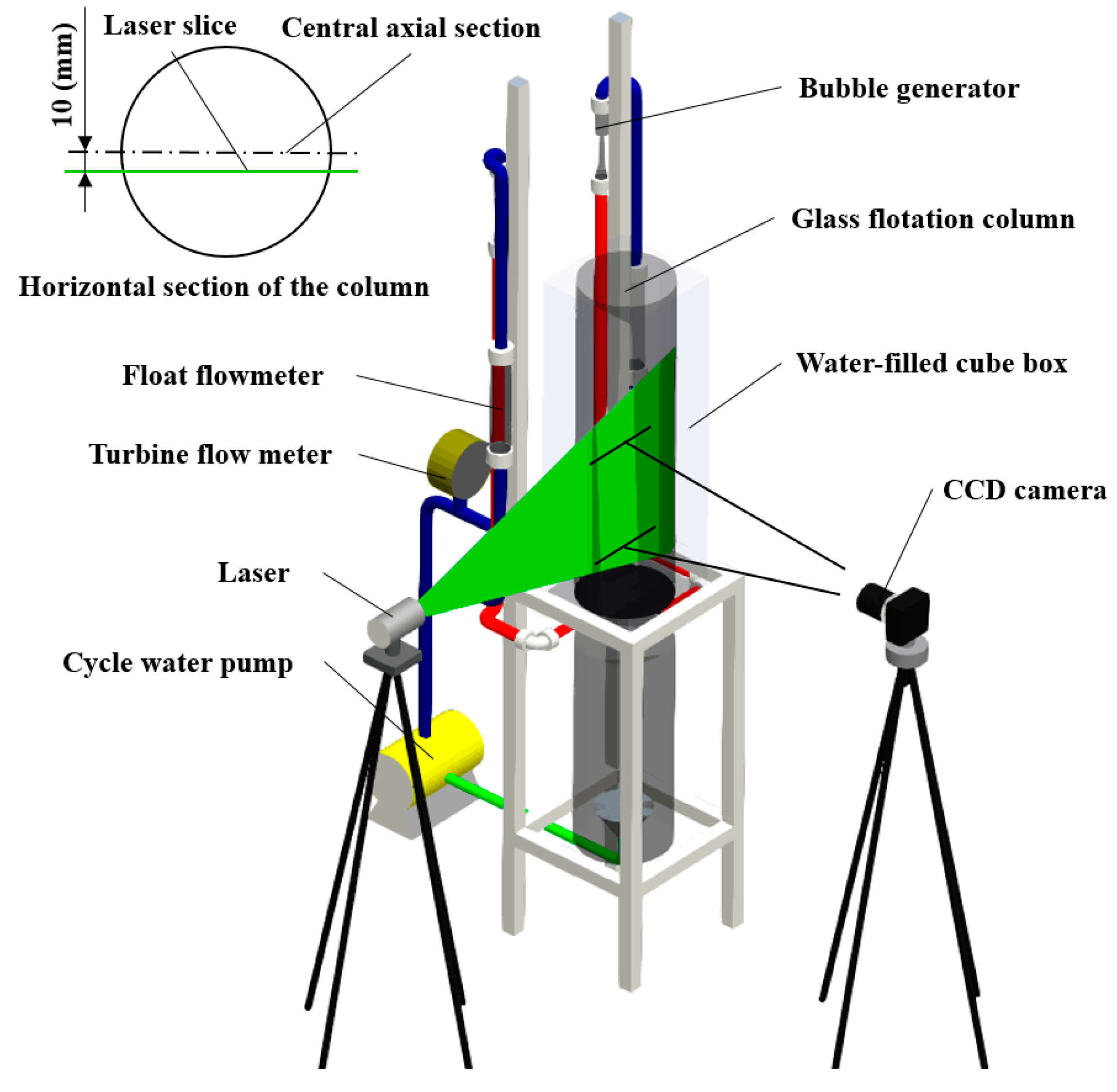
Figure 3 shows how the laser light sheet, CCD camera, and test sections were placed to measure the flotation column axial section. Several bubbles clustered near the column axis, which would interfere with the laser light sheet, reduce the flow field and luminance at the axis and in the other half of the flotation column, impacting measurement accuracy. This approach is similar to that employed by Wang et al. [10]. Therefore, following some initial experiments, we adopted the quasi-axial section, deviating 10 mm from the central axial section as the measurement plane to ensure more accurate experimental data, as shown in the dash-solid section in Figure 3 (260–340 mm above the inverted cone). The left side was illuminated by laser with sufficient intensity. Four circulating flow types were selected for experiments, considering industrial applications. Table 1 shows optimal experimental parameters derived from several trial experiments and adjustments, and we averaged 200 photograph pairs. Experimental data at 300 mm height was extracted for comparison with CFD simulations.
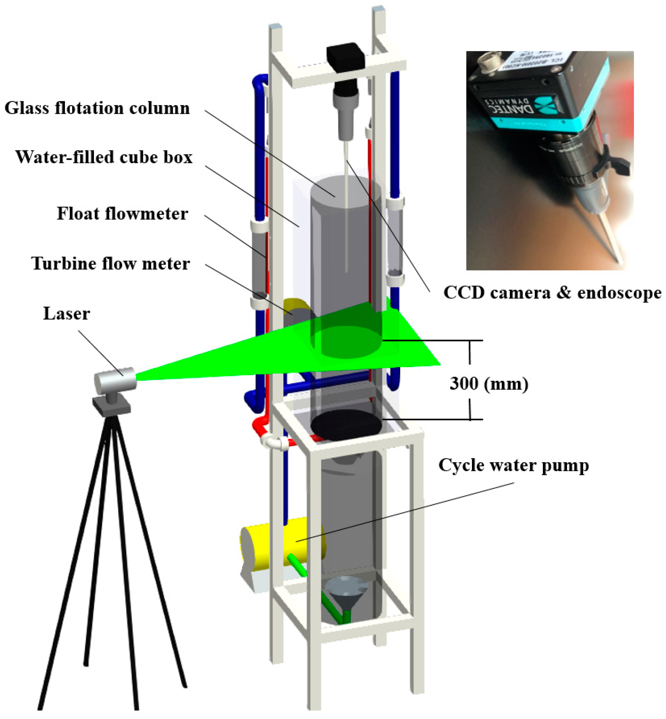
To obtain tangential velocity, we installed the CCD camera above the column, providing downward looking images to measure the horizontal section. However, the water swirls when the flotation column is in operation, and the free surface between air and water inside the column flotation zone, forms an inverted cone. Laser-illuminated tracer particles are refracted when passing through this free surface, causing deviations in the CCD images. To solve this problem, we employed an endoscope for the PIV test, allowing the lens to be inserted into the water to test the flow field, and hence eliminating most optical interference. Velarde [16] and Helmi [17] used an endoscopic laser PIV technique for dense gas–solid fluidized beds in 2016 and 2018, respectively, which inspired the current proposed PIV measurement system for cyclonic flow fields in the flotation column.
Figure 4 shows how an endoscope was installed onto the CCD camera and extended below the free surface. The measured horizontal section was 300 mm above the inverted cone. Table 2 shows optimal experimental parameters derived from many preliminary experiments, with 200 photograph pairs captured for averaging. Similar to flotation column axial section measurements discussed above, we selected data along a straight line in the radial direction, and the same four circulating flows were employed, as shown in Table 2.

3. Numerical Simulation

3.1. Turbulence Models

Turbulence models greatly impact results from single-phase numerical simulations (Table 3). Turbulence model expression establishment and application differ, producing inconsistent predictions for many flow field types. We compared the RSM, standard k-ε model, realizable k-ε model, and RNG k-ε models. As one of the most widely used turbulence models, the standard k-ε model is based on transport equations for turbulent kinetic energy, k, and its dissipation rate, ε [18], which are defined as
( ρ k ) t + ( ρ k u i ) x i = x j [ ( μ + μ t σ k ) k x j ] + G k + G b ρ ε Y M + S k ,
( ρ ε ) t + ( ρ ε u i ) x i = x j [ ( μ + μ t σ ε ) ε x j ] + C 1 ε ε k ( G k + C 3 ε G b ) C 2 ε ρ ε 2 k + S ε .
The RNG k-ε model was proposed by Yakhot and Orzga [19] in 1986. It is similar in form to the standard k-ε model, but includes some refinements. The RNG model has an additional term in its equation that improves the accuracy for rapidly strained flows. In addition, the effect of swirl on turbulence is included in the model, enhancing accuracy for swirling flows. What is more, it provides an analytical formula for turbulent Prandtl numbers, while the standard k-ε model uses user-specified, constant values. Therefore, these features make the RNG k-ε model more accurate and reliable for a wider class of flows than the standard k-ε model. The equations are given as:
( ρ k ) t + ( ρ k u i ) x i = x j [ a k μ e f f k x j ] + G k + G b ρ ε Y M + S k ,
( ρ ε ) t + ( ρ ε u i ) x i = x j ( a ε μ e f f ε x j ) + C 1 ε ε k ( G k + C 3 ε G b ) C 2 ε ρ ε 2 k R ε + S ε .
The realizable k-ε model was proposed by Moin et al. [20] who believe that the standard k-ε model may cause stress errors when the time-averaged strain rate is strong. The model [21] implements an alternative formulation for turbulent viscosity [22] based on a modified transport equation for dissipation derived from an exact equation for mean-square vorticity fluctuation transportation:
( ρ k ) t + ( ρ k u j ) x j = x j [ ( μ + μ t σ k ) k x j ] + G k + G b ρ ε Y M + S k ,
( ρ ε ) t + ( ρ ε u j ) x j = x j [ ( μ + μ t σ ε ) ε x j ] + ρ C 1 E ε ρ C 2 ε 2 k + ν ε + C 1 ε ε k C 3 ε G b + S ε .
RSM closes the Reynolds-averaged Naiver–Stokes equations by abandoning the isotropic eddy-viscosity hypothesis and solving transport equations for Reynolds stresses, together with an equation for the dissipation rate [23,24,25]. The control equations are as follows:
Continuity equations:
ρ t + ( ρ u i ) = 0 .
Momentum equation:
u i t + x j ( u i u j ) = 1 ρ p x i + 1 ρ x j [ μ ( u i x j + u j x i ) ] + x j ( u i u j ¯ ) ,
where
u i = u i ¯ + u i .
Turbulence production term P i j is defined as
P i j = ρ ( u i u k ¯ u j x k + u j u k ¯ u j x k ) .
Turbulence dissipation rate ε i j is given as
ε i j = 2 μ u i x k u j x k ¯ .
Press strain φ i j is defined as
φ i j = p ( u i x j + u j x i ) ¯ .
Turbulence diffusion D T , i j is given as
D T , i j = x k ( ρ u i u j u k ¯ + p u i ¯ δ j k μ x k u i u j ¯ ) .

3.2. Geometry and Mesh

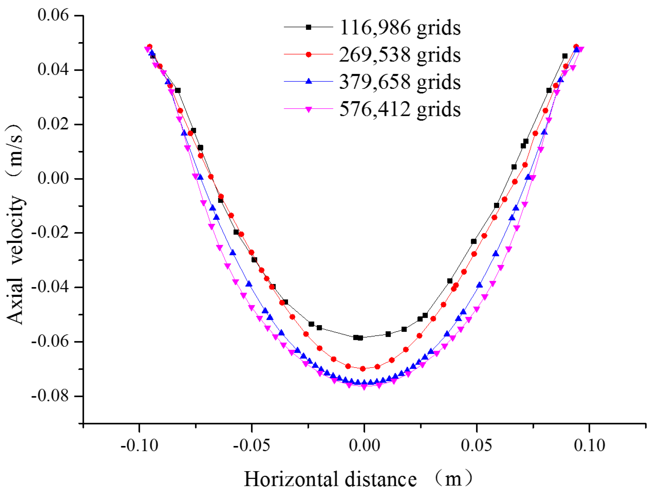
The 3D FCSMC model was established for the experimental device, as shown in Figure 5, and geometric model processing was consistent with Wang et al. [10] and Yan et al. [13]. A structured mesh was constructed aside from the inverted cone, which was unstructured mesh (see Figure 5), and grid independence was verified. Figure 6 shows axial velocity along the horizontal direction at 300 mm column height for different mesh schemes. We selected a model incorporating 379,658 grids.

3.3. Boundary Conditions and Solution

In order to match the numerical simulation with the PIV experiment, we set the boundary conditions according to the experiment. Two tangential inlets (Figure 5, Inlet 1 and 2) in the cyclonic unit are defined as velocity inlets, with fluid speeds of 0.11, 0.22, 0.44, and 0.66 m/s for 0.25, 0.50, 1.00, and 1.50 m3/h flow rates, respectively. Since the fluid was single phase, we assumed that all feed was discharged from the middling port, with the amount of feed equal to the amount of discharge. Therefore, the middling port outlet was defined as a negative velocity inlet with 0.22, −0.44, −0.88, and −1.32 m/s, respectively. The acceleration of gravity is 9.81 m/s, which is vertically downward along the axis. Table 4 shows all boundary conditions and calculation values.
Commercial CFD code ANSYS Fluent was employed to carry out the simulation. We used the SIMPLE algorithm for pressure–velocity coupling, the least squares cell based on gradient, the PRESTO! scheme for pressure discretization, and the second order upwind scheme for momentum discretization, turbulent kinetic energy, turbulent dissipation rate, and Reynolds stresses. The calculation used an unsteady solver, hence once the parameters and residuals of the monitored point reached statistical stability, the results of the previous 20 s duration were averaged and used for subsequent analysis.

3.4. CFD and PIV Comparison

3.4.1. Velocity Vectors

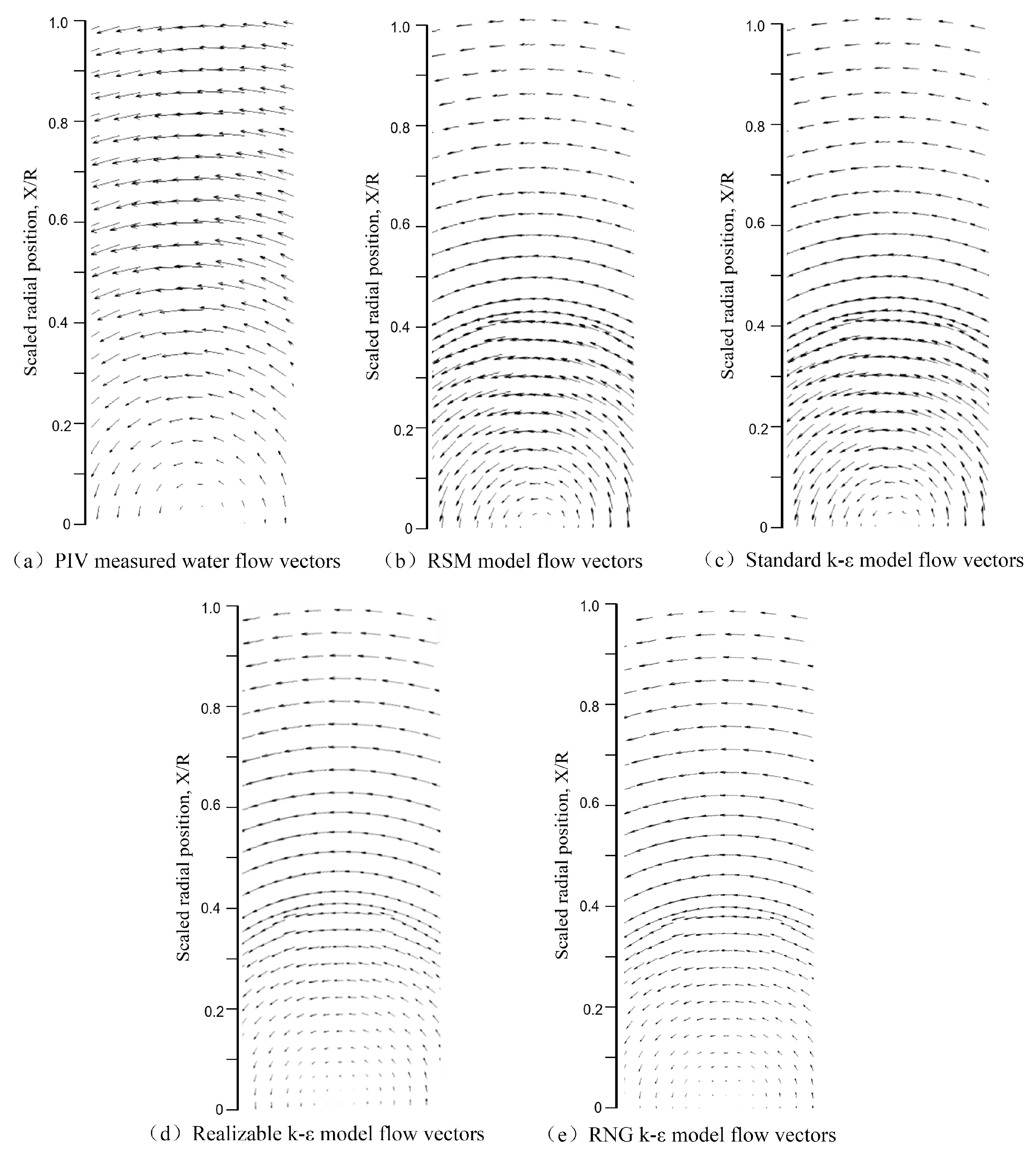
Figure 7a shows the vertical PIV experimental vectors located at the plane 260–340 mm above the inverted cone and parallel to the 10 mm axial section. Simulation and PIV results were compared at 1.00 m3/s to verify prediction accuracy. PIV showed gradually increasing water vector magnitude as distance from the column wall increased, followed by a sharp reduction, with water flowing approximately horizontally toward the axis. Figure 7b shows that RSM model vectors were consistent with the PIV results, whereas other models (Figure 7c–e) produced divergent directions close to the axis, being diagonally downwards.
Figure 8 compares PIV (Figure 8a) and model (Figure 8b–e) results for the horizontal plane 300 mm above the inverted cone. All the models are consistent with PIV in that the water rotates counterclockwise around the center.

3.4.2. Quantitative Analysis

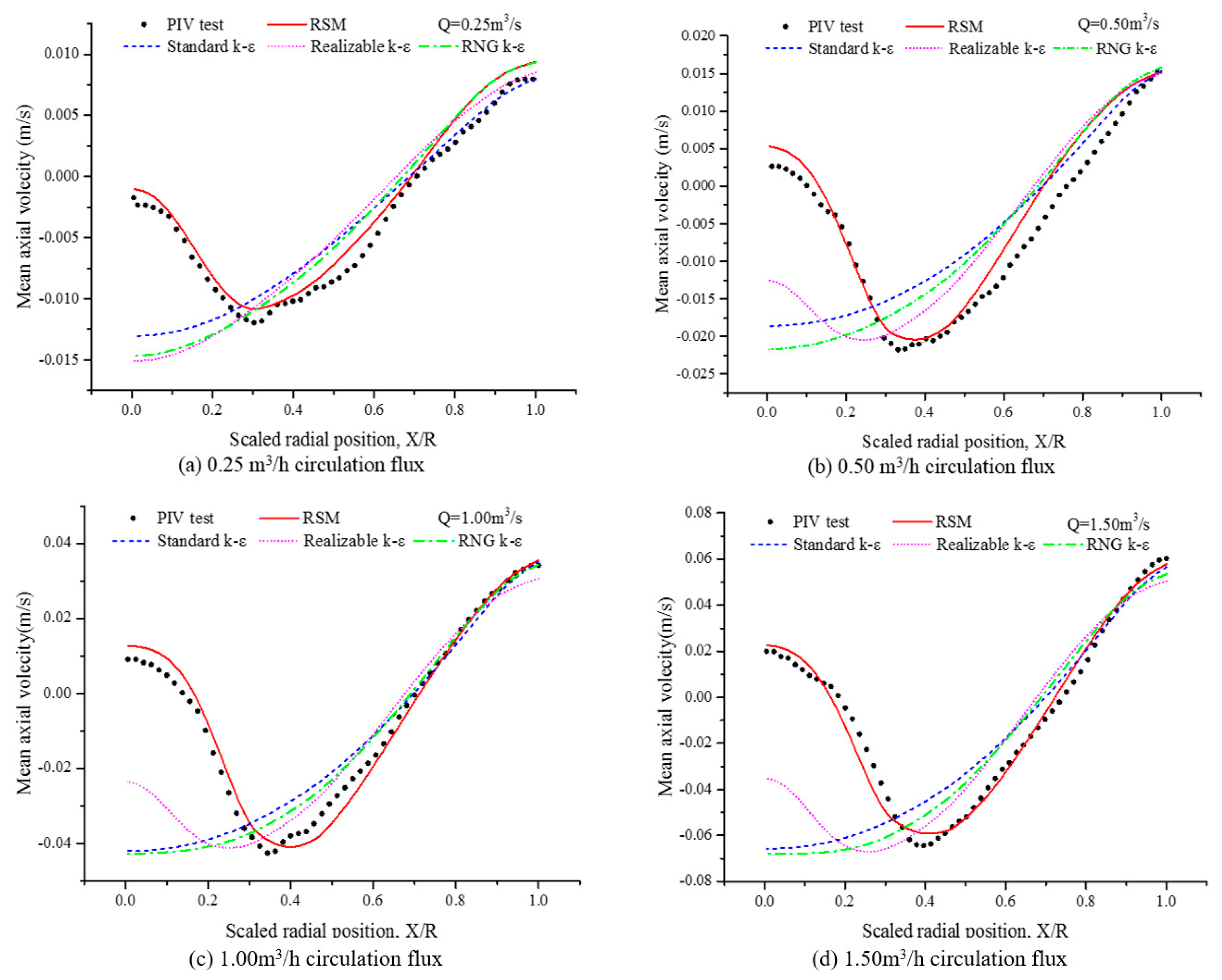
Figure 9 and Figure 10 compare the simulated and measured velocity profiles along the horizontal direction for a cyclic flux of 0.25, 0.50, 1.00, and 1.50 m3/h, respectively, at z = 300 mm, 10 mm off-axis. As for Figure 11, the velocity distribution of the simulation and measurement in the horizontal direction from the axis to the wall at z = 300 mm is compared. The RSM and realizable k-ε turbulent model axial velocity distribution trends exhibit the in “√” shape, consistent with PIV results. However, the standard k-ε and RNG k-ε model trends diverge widely.
Figure 10 and Figure 11 show radial and tangential velocity results, respectively. Distribution trends along the horizontal direction are consistent with PIV results for all turbulence models.
Thus, RSM and realizable k-ε models exhibit good prediction performance for velocity distributions in all directions, whereas the standard k-ε model and the RNG k-ε model can only predict velocity distribution trends in radial and tangential directions.
Table 5, Table 6 and Table 7 summarize absolute deviations between simulation and PIV results (excluding data within 3 mm of the zero velocity point) for axial, radial, and tangential velocities, respectively. Since the standard k-ε model and the RNG k-ε model cannot predict velocity distribution trends in the axial direction, only radial and tangential errors were analyzed. The RSM model achieved the smallest error for all directions.
The k-ε models are based on isotropic assumptions with semi-empirical formulas summarized from experimental results. However, the high-intensity swirling field has a large turbulent velocity gradient and fluctuating turbulent velocity, and hence is not even approximately isotropic. Therefore, k-ε models are less effective, and the swirling flow field inside the flotation column cannot be correctly modelled. The RSM model is the most accurate model among the four models considered. This model abandons the isotropic assumption, considering laminar flow and Reynolds stress, and hence is suitable for anisotropic cases.

4. Conclusions

We performed numerical simulations and PIV measurements for a single-phase swirling field in a lab-scale FCSMC at four circulation fluxes (0.25, 0.50, 1.00, and 1.50 m3/h). Axial and radial velocity distributions were measured and modelled on the flotation column quasi-axial section. Experimental errors due to refraction at the free surface were avoided by adding an endoscopic lens to the CCD camera, inserting the speculum below the free surface, and allowing tangential velocity distribution to be measured on the indicated section. The RSM, standard k-ε model, realizable k-ε model, and RNG k-ε model were used for CFD simulations for FCSMC single-phase swirling fields. Comparing the PIV experimental and simulation results and of the PIV, we made the following conclusions:
(1) Standard k-ε model and RNG k-ε model. Radial and tangential velocity distribution trends simulated by these models were consistent with PIV measurements, but axial velocity along the horizontal direction deviated widely from PIV results. Thus, axial errors were not considered. Mean absolute radial and tangential velocity deviations were 37.25% and 38.92%, for the standard k-ε model and slightly better for the RNG k-ε model (32.82% and 29.60%), respectively.
(2) RSM and realizable k-ε model. Radial, tangential, and axial velocity distribution trends simulated by these models were all consistent with PIV measurements. Mean absolute axial, radial, and tangential velocity deviations were 17.36%, 14.79%, and 13.48% for the RSM model, and 78.11%, 28.94%, and 26.12% for the realizable k-ε model, respectively. Therefore, the RSM model exhibited superior performance, particularly in the axial direction.
(3) The k-ε models [26] are based on isotropic assumptions with semi-empirical formulas summarized from experimental results. However, the internal flow field of the flotation column is a high-intensity vortex field with a large turbulent velocity gradient and fluctuating turbulent velocity, and hence is not approximately isotropic. The RSM model [27] abandons the isotropic assumption, considering laminar flow and Reynolds stress, and hence is suitable for anisotropic cases, especially the swirling flow field inside the flotation column. In fact, the RANS (Reynolds Averaged Navier-Stokes) model [28] does not distinguish between the size and direction of the vortex, and it is limited by the model conditions. Thus, it is difficult to get perfect results for complex problems such as an inverse pressure gradient numerical simulation. In addition, the RANS model relies on boundary conditions, so the calculations are very computationally dependent. DNS and even LES are good choices without considering computational costs and widespread adoption.
Author Contributions

Conceptualization, X.Y., Y.C.; methodology, S.M., L.W.; software, S.M., X.L.; validation, X.L.; investigation, H.Z.; data curation, S.M., X.Y.; writing-original draft preparation, S.M.; writing-review and editing, S.M., X.Y.; visualization, S.M., X.L.; and funding, Y.C., H.Z., L.W.

Funding

This research was funded by the National Natural Science Foundation of China (U1704252), the Fundamental Research Funds for the Central Universities (2017XKZD02) and the National Natural Science Foundation of China (51722405).

Conflicts of Interest

The authors declare no conflict of interest.

References

  1. Jiongtian, L. Cyclonic-Static Micro-Bubble Floatation Apparatus and Method. U.S. Patent 6073775, 19 January 1999. [Google Scholar]
  2. Tian, J.; Ni, L.; Song, T.; Olson, J.; Zhao, J. An overview of operating parameters and conditions in hydrocyclones for enhanced separations. Sep. Purif. Technol. 2018, 206, 268–285. [Google Scholar] [CrossRef]
  3. Li, X.; Xu, H.; Liu, J.; Zhang, J.; Li, J.; Gui, Z. Cyclonic state micro-bubble flotation column in oil-in-water emulsion separation. Sep. Purif. Technol. 2016, 165, 101–106. [Google Scholar] [CrossRef]
  4. Zhang, H.; Liu, J.; Wang, Y.; Cao, Y.; Ma, Z.; Li, X. Cyclonic-static micro-bubble flotation column. Miner. Eng. 2013, 45, 1–3. [Google Scholar] [CrossRef]
  5. Guichao, W.; Linhan, G.; Subhasish, M.; Evans, G.M.; Joshi, J.B.; Songying, C. A review of CFD modelling studies on the flotation process. Miner. Eng. 2018, 127, 153–177. [Google Scholar]
  6. Buchhave, P. Particle image velocimetry—Status and trends. Exp. Therm. Fluid Sci. 1992, 5, 586–604. [Google Scholar] [CrossRef]
  7. Marins, L.P.M.; Duarte, D.G.; Loureiro, J.B.R.; Moraes, C.A.C.; Freire, A.P.S. LDA and PIV characterization of the flow in a hydrocyclone without an air-core. J. Pet. Sci. Eng. 2010, 70, 168–176. [Google Scholar] [CrossRef]
  8. Cui, B.Y.; Wei, D.Z.; Gao, S.L.; Liu, W.G.; Feng, Y.Q. Numerical and experimental studies of flow field in hydrocyclone with air core. Trans. Nonferr. Met. Soc. China 2014, 24, 2642–2649. [Google Scholar] [CrossRef]
  9. Yan, X.; Meng, S.; Wang, A.; Wang, L.; Cao, Y. Hydrodynamics and separation regimes in a cyclonic-static microbubble flotation column. Asia Pac. J. Chem. Eng. 2018, 13, e2185. [Google Scholar] [CrossRef]
  10. Wang, A.; Yan, X.; Wang, L.; Cao, Y.; Liu, J. Effect of cone angles on single-phase flow of a laboratory cyclonic-static micro-bubble flotation column: PIV measurement and CFD simulations. Sep. Purif. Technol. 2015, 149, 308–314. [Google Scholar] [CrossRef]
  11. Khan, Z.; Bhusare, V.H.; Joshi, J.B. Comparison of turbulence models for bubble column reactors. Chem. Eng. Sci. 2017, 164, 34–52. [Google Scholar] [CrossRef]
  12. Zhang, M.; Li, T.; Wang, G. A CFD study of the flow characteristics in a packed flotation column: Implications for flotation recovery improvement. Int. J. Miner. Process. 2017, 159, 60–68. [Google Scholar] [CrossRef]
  13. Yan, X.; Liu, J.; Cao, Y.; Wang, L. A single-phase turbulent flow numerical simulation of a cyclonic-static micro bubble flotation column. Int. J. Min. Sci. Technol. 2012, 22, 95–100. [Google Scholar] [CrossRef]
  14. Swain, S.; Mohanty, S. A 3-dimensional Eulerian–Eulerian CFD simulation of a hydrocyclone. Appl. Math. Model. 2013, 37, 2921–2932. [Google Scholar] [CrossRef]
  15. Azadi, M.; Azadi, M.; Mohebbi, A. A CFD study of the effect of cyclone size on its performance parameters. J. Hazard. Mater. 2010, 182, 835–841. [Google Scholar] [CrossRef] [PubMed]
  16. Velarde, I.C.; Gallucci, F.; Annaland, M.V.S. Development of an endoscopic-laser PIV/DIA technique for high-temperature gas–solid fluidized beds. Chem. Eng. Sci. 2016, 143, 351–363. [Google Scholar] [CrossRef]
  17. Helmi, I.C.V.A.; Gallucci, F.; van Sint Annaland, M. Hydrodynamics of dense gas-solid fluidized beds with immersed vertical membranes using an endoscopic-laser PIV/DIA technique. Chem. Eng. Sci. 2018, 182, 146–161. [Google Scholar] [CrossRef]
  18. Spalding, B.D. Lectures in Mathematical Models of Turbulence; Academic Press: Cambridge, MA, USA, 1972. [Google Scholar]
  19. Victor Yakhot, S.A.O. Renormalization group analysis of turbulence: Basic theory. J. Sci. Comput. 1986, 1, 3–11. [Google Scholar] [CrossRef]
  20. Peinke Moin, J.K.; Gerrit, O. Progress in Large Eddy Simulation of Turbulent Flows; AIAA Paper 97-15761; American Institute of Aeronautics and Astronautics: Reston, VA, USA, 1997. [Google Scholar]
  21. Shih, T.H.; Liou, W.W.; Shabbir, A.; Yang, Z.; Zhu, J. A New Kappa-Epsilon Eddy Viscosity Model for high Reynolds Number Turbulent Flows-Model Development and Validation; Linthicum Heights Md Nasa Center for Aerospace Information |c: Linthicum Heights, MD, USA, 1995. [Google Scholar]
  22. Orszag, S.A.; Yakhot, V.; Flannery, W.S.; Boysan, F.; Choudhury, D.; Maruzewski, J.; Patel, B. Renormalization Group Modeling and Turbulence Simulations; Elsevier: Amsterdam, The Netherlands, 1993. [Google Scholar]
  23. Launder, B.E.; Reece, G.J.; Rodi, W. Progress in the development of a Reynolds-stress turbulence closure. J. Fluid Mech. 1975, 68, 537–566. [Google Scholar] [CrossRef] [Green Version]
  24. Launder, B.E. Second-moment closure: Present … and future? Int. J. Heat Fluid Flow 1989, 10, 282–300. [Google Scholar] [CrossRef]
  25. Gibson, M.M.; Launder, B.E. Ground effects on pressure fluctuations in the atmospheric boundary layer. J. Fluid Mech. 2006, 86, 491–511. [Google Scholar] [CrossRef]
  26. Mendoza-Escamilla, V.X.; Alonzo-García, A.; Mollinedo, H.R.; González-Neria, I.; Yáñez-Varela, J.A.; Martinez-Delgadillo, S.A. Assessment of k-ε models using tetrahedral grids to describe the turbulent flow field of a PBT impeller and validation through the PIV technique. Chin. J. Chem. Eng. 2018, 26, 942–956. [Google Scholar]
  27. Khan, Z.; Joshi, J.B. Comparison of k–ε, RSM and LES models for the prediction of flow pattern in jet loop reactor. Chem. Eng. Sci. 2015, 127, 323–333. [Google Scholar] [CrossRef]
  28. Xiao, H.; Cinnella, P. Quantification of Model Uncertainty in RANS Simulations: A Review. Prog. Aerosp. Sci. 2019, 108, 1–31. [Google Scholar] [CrossRef]
Figure 1. Typical cyclonic static microbubble flotation column structure.
Minerals 09 00464 g001
Figure 2. Forces and interactions inside an operating flotation column.
Minerals 09 00464 g002
Figure 3. Particle image velocimetry (PIV) measurement of a quasi-axial section.
Minerals 09 00464 g003
Figure 4. Horizontal section PIV measurement.
Minerals 09 00464 g004
Figure 5. Flotation column 3D model (a) and mesh (b).
Minerals 09 00464 g005
Figure 6. Grid independence: The curve of axial velocity along the horizontal direction on a section 300 mm above the inverted cone at 1.50 m3/h flux.
Minerals 09 00464 g006
Figure 7. Experimental and simulation water flow vectors in quasi-axis sections. (a) PIV measured water flow vectors; (b) RSM model flow vectors; (c) Standard k-ε model flow vectors; (d) Realizable k-ε model flow vectors; (e) RNG k-ε model flow vectors.
Minerals 09 00464 g007
Figure 8. Experiment model water flow vectors in horizontal sections. (a) PIV measured water flow vectors; (b) RSM model flow vectors; (c) Standard k-ε model flow vectors; (d) Realizable k-ε model flow vectors; (e) RNG k-ε model flow vectors.
Minerals 09 00464 g008
Figure 9. Axial velocity distribution calculated by turbulence models and PIV measurement along the horizontal direction, 300 mm high, and 10 mm from the axial section.
Minerals 09 00464 g009
Figure 10. Radial velocity distribution calculated by turbulence models and PIV measurement along the horizontal direction, 300 mm high, and 10 mm from the axial section.
Minerals 09 00464 g010
Figure 11. Tangential velocity distribution calculated by turbulence models and PIV measurement along the horizontal direction, 300 mm high.
Minerals 09 00464 g011
Table 1. PIV experimental parameters for cyclonic static microbubble flotation column vertical sections.
Measuring SurfaceRecycling Flow (m3/h)Measurement ParametersLaser Interval (μs)Trigger Frequency
Vertical section, 260–340 mm above the cyclonic flotation unit0.25Axial velocity, radial velocity12009.0 Hz
0.50800
1.00600
1.50300
Table 2. Cyclonic static microbubble flotation column (FCSMC) horizontal section PIV measurement parameters.
Measuring SurfaceRecycling Flow (m3/h)Measurement ParameterLaser Interval (μs)Trigger Frequency
Column cross-section, 300 mm above the column flotation unit0.25Tangential velocity10009.0 Hz
0.50600
1.00400
1.50200
Table 3. Symbol and interpretation.
SymbolInterpretationSymbolInterpretation
k Turbulence kinetic energy φ Press strain
ε Turbulence dissipation rate D Turbulence diffusion
ρ Density p Pressure
u Velocity μ Viscosity
C Constant t Time
P Turbulence production term δ Kronecker delta function
i , 1 x component j , 2 y component
k , 3 z component (in the RSM) S k , S ε User-defined source terms.
G k The generation of turbulence kinetic energy due to the mean velocity gradients, calculated as described in Modeling Turbulent Production in the k-ε Models.
G b The generation of turbulence kinetic energy due to buoyancy, calculated as described in Effects of Buoyancy on Turbulence in the k-ε Models.
Y M The contribution of the fluctuating dilatation in compressible turbulence to the overall dissipation rate, calculated as described in Effects of Compressibility on Turbulence in the k-ε Models.
σ k , σ ε The turbulent Prandt1 numbers for k and ε.
Table 4. Circulation flow boundary conditions.
BoundaryTypeCirculating Volume Rate (m3/h)
0.250.501.001.50
Inlet 1Inlet velocity (m/s)0.110.220.440.66
Inlet 2Inlet velocity (m/s)0.110.220.440.66
Concentrate outletSymmetry----
Middling port outletInlet velocity (m/s)−0.22−0.44−0.88−1.32
Table 5. Simulation model axial velocity absolute deviation from PIV measurement.
Flow Rate (m3/h)Turbulence Model
RSM (%)Standard k-ε (%)Realizable k-ε (%)RNG k-ε (%)
0.2519.8987.12106.15102.86
0.5018.7671.8768.4280.11
1.0014.3990.4267.2286.85
1.5016.3983.5870.6588.26
Mean absolute deviation17.3683.2578.1189.52
Table 6. Simulation model radial velocity absolute deviation from PIV measurement.
Flow Rate (m3/h)Turbulence Model
RSM (%)Standard k-ε (%)Realizable k-ε (%)RNG k-ε (%)
0.2511.5441.3330.8231.89
0.5018.2338.4230.5031.29
1.0013.5537.1729.2431.56
1.5015.8632.0625.2036.54
Mean absolute deviation14.7937.2528.9432.82
Table 7. Simulation model tangential velocity absolute deviation from PIV measurement.
Flow Rate (m3/h)Turbulence Model
RSM (%)Standard k-ε (%)Realizable k-ε (%)RNG k-ε (%)
0.2516.8746.8427.3932.86
0.5013.8737.7427.8830.79
1.0010.3936.4924.6128.14
1.5012.7734.6024.6026.61
Mean absolute deviation13.4838.9226.1229.60