Prospectivity Mapping of Mineral Deposits in Northern Norway Using Radial Basis Function Neural Networks


Abstract
1. Introduction
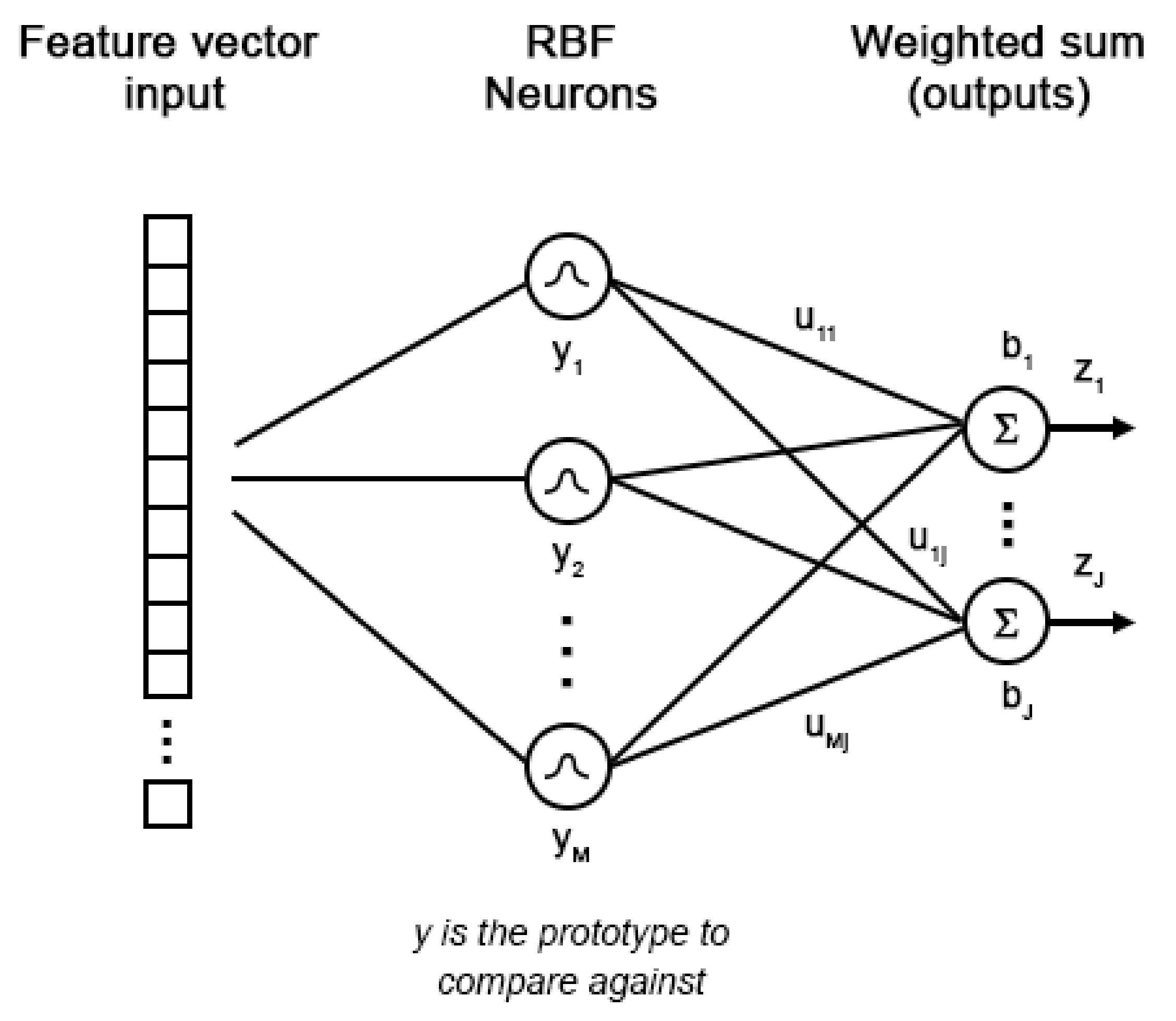
2. Radial Basis Function Neural Networks (RBFNN)
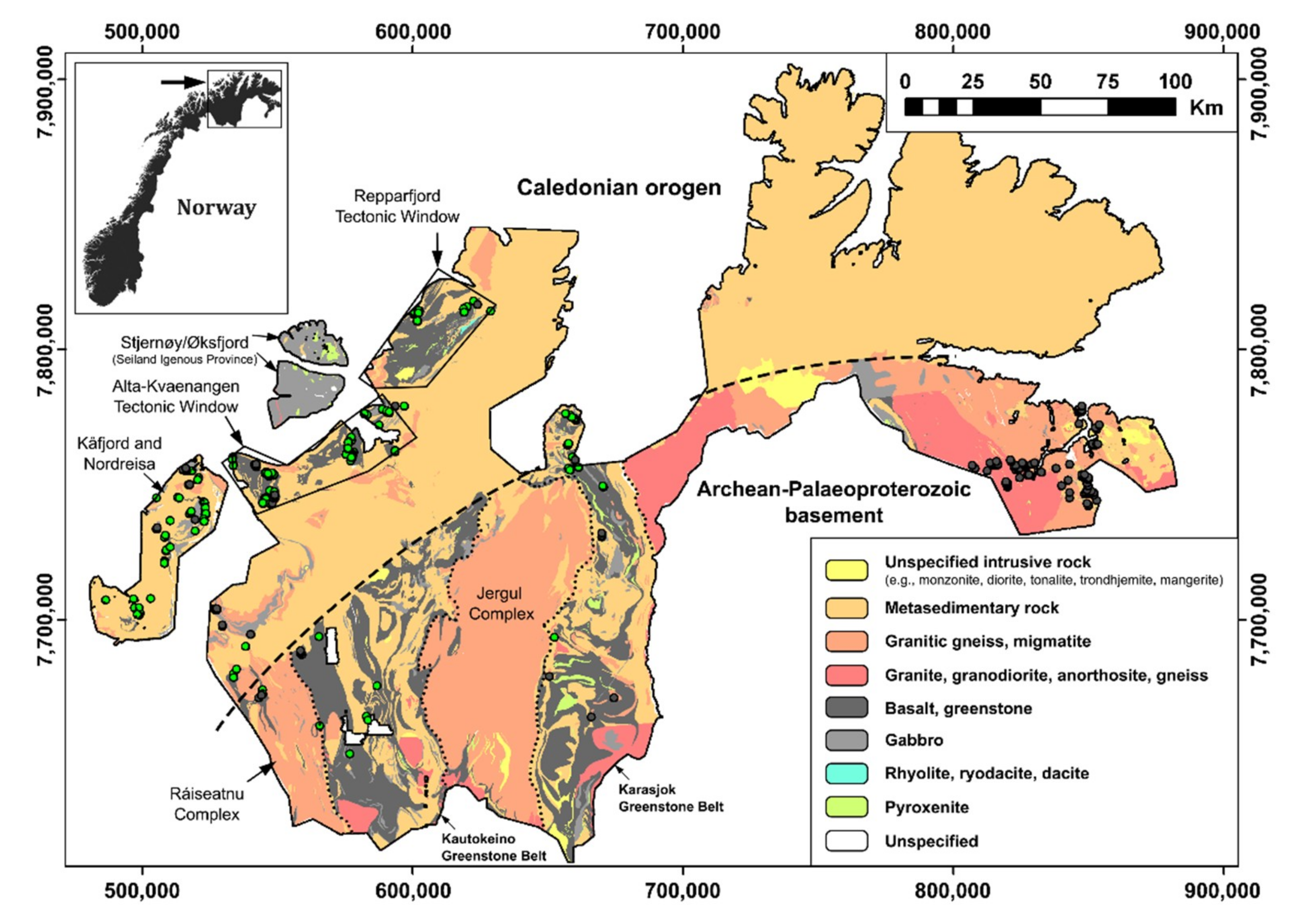
3. Regional Geology and Mineralization
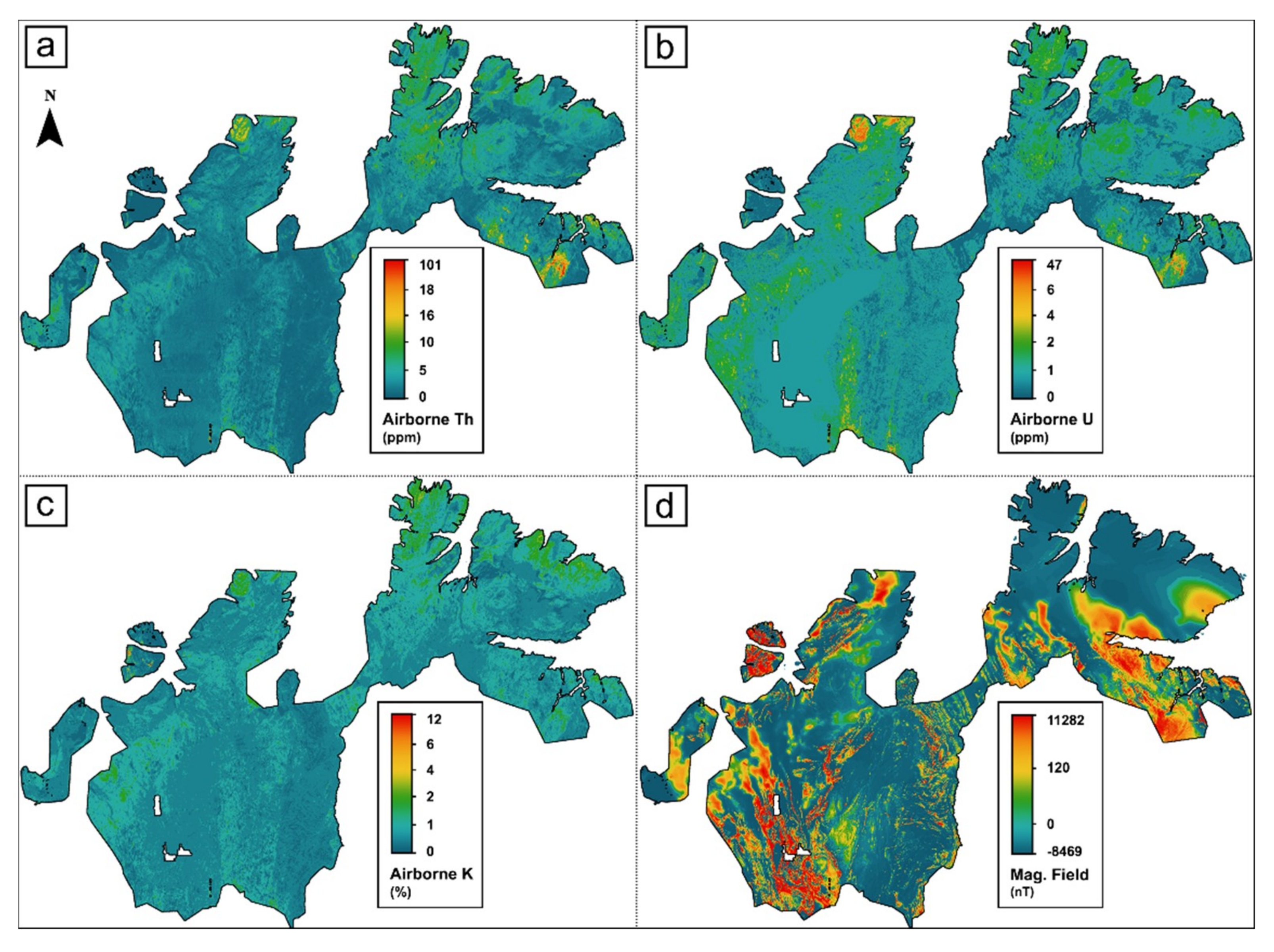
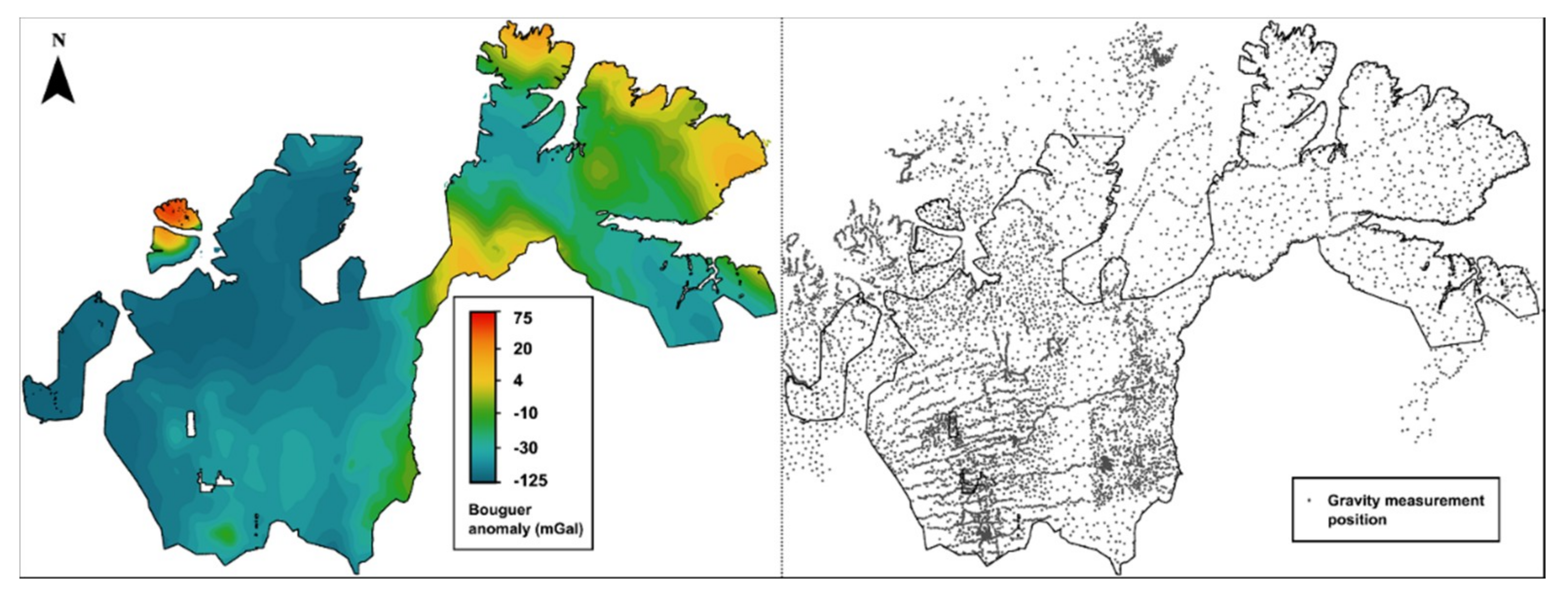
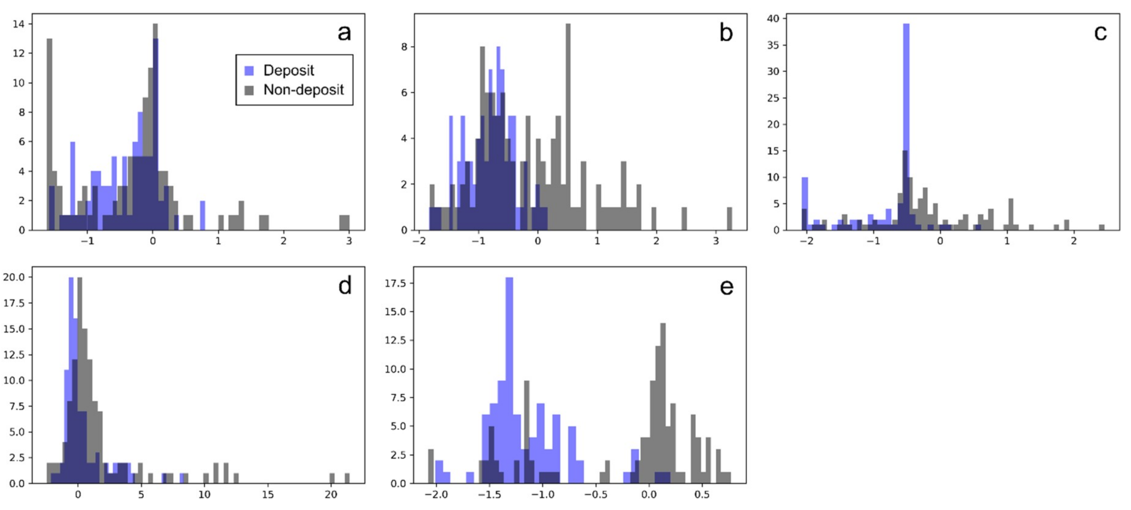
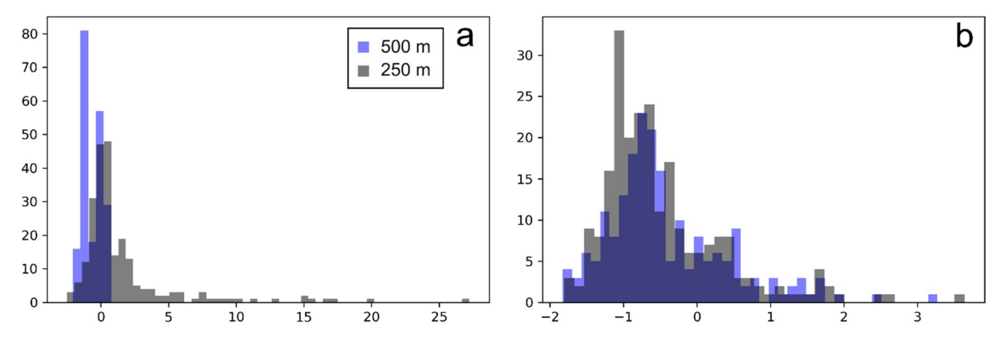
4. Data Processing
5. Network Implementation
5.1. Architecture and Training Phase
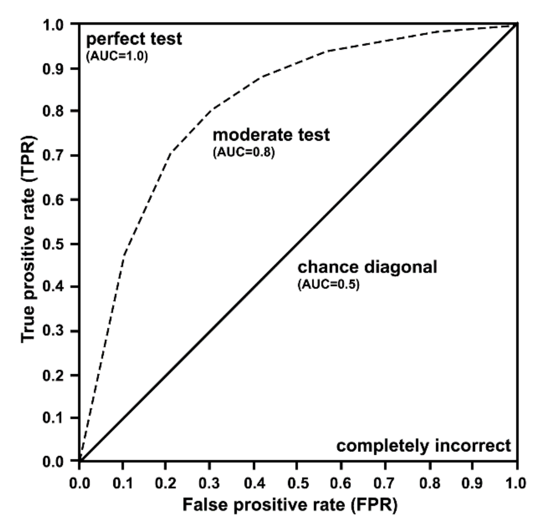
5.2. Metrics
6. Results and Discussion
6.1. Training and Validation
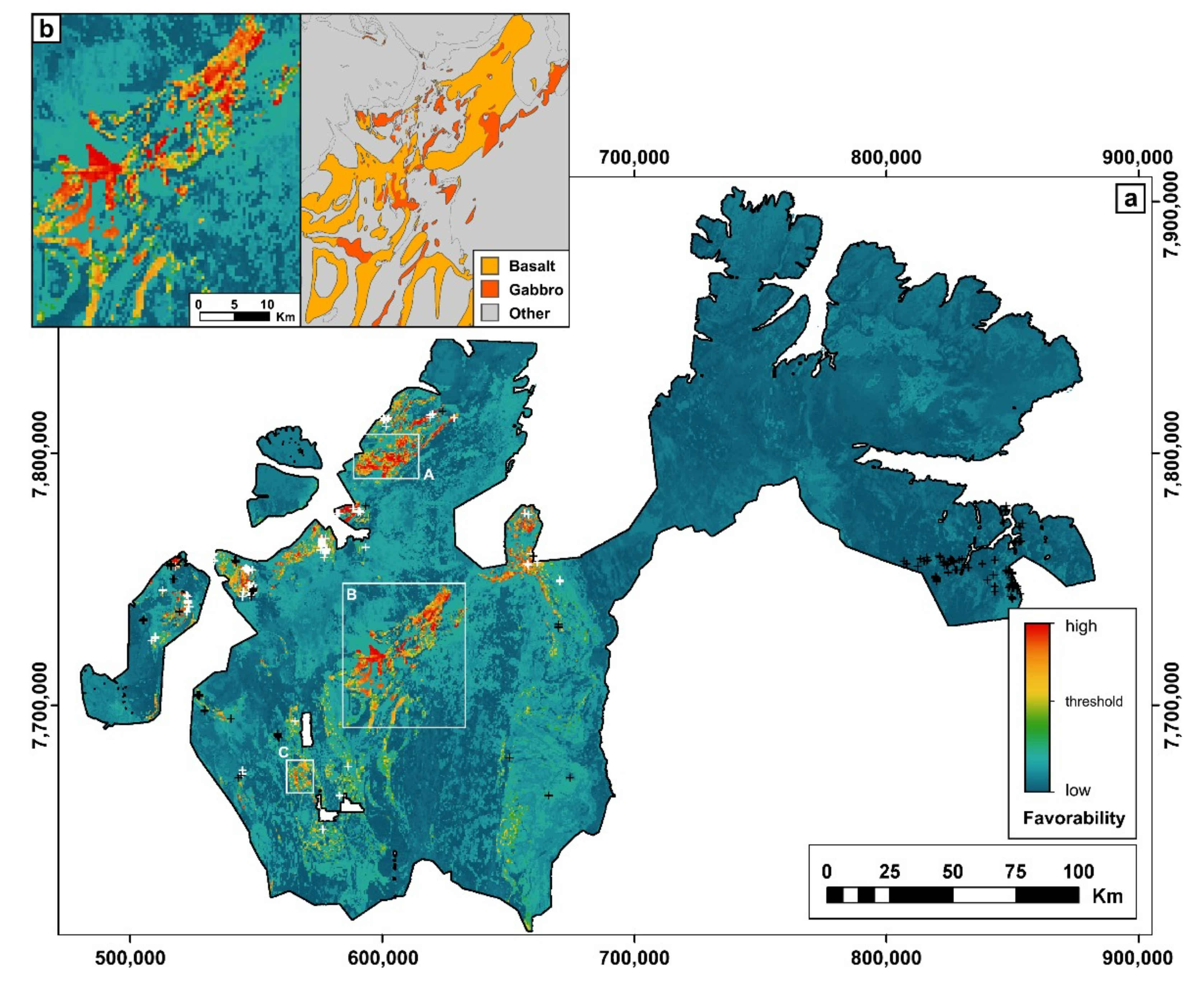
6.2. Classification and Limitations
7. Conclusions
Author Contributions
Funding
Conflicts of Interest
Appendix A.


References
- Porwal, A.K.; Carranza, E.J.M.; Hale, M. Artificial Neural Networks for Mineral-Potential Mapping: A Case Study from Aravalli Province, Western India. Nat. Resour. Res. 2003, 12, 155–171. [Google Scholar] [CrossRef]
- Porwal, A.K. Mineral Potential Mapping with Mathematical Geological Models. Ph.D. Thesis, University of Utrecht, Utrecht, The Netherlands, 2006. [Google Scholar] [CrossRef]
- Behnia, P. Application of Radial Basis Functional Link Networks to Exploration for Proterozoic Mineral Deposits in Central Iran. Nat. Resour. Res. 2007, 16, 147–155. [Google Scholar] [CrossRef]
- Nykänen, V. Radial Basis Functional Link Nets Used as a Prospectivity Mapping Tool for Orogenic Gold Deposits Within the Central Lapland Greenstone Belt, Northern Fennoscandian Shield. Nat. Resour. Res. 2008, 17. [Google Scholar] [CrossRef]
- Singer, D.A.; Kouda, R. Application of a Feedforward Neural Network in the Search for Kuroko Deposits in the Hokuroku District, Japan. Math. Geol. 1996, 28. [Google Scholar] [CrossRef]
- Singer, D.A.; Kouda, R. Use of a Neural Network to Integrate Geoscience Information in the Classification of Mineral Deposits and Occurrences. Integrated Exploration Information Management. In Proceedings of the Exploration 97: Fourth Decennial International Conference on Mineral Exploration, Toronto, ON, Canada, 14–18 September 1997; pp. 127–134. [Google Scholar]
- Harris, D.-V.; Pan, G. Mineral Favorability Mapping: A Comparison of Artificial Neural Networks, Logistic Regression, and Discriminant Analysis. Nat. Resour. Res. 1999, 8, 93–109. [Google Scholar] [CrossRef]
- Brown, W.M.; Gedeon, T.D.; Groves, D.I.; Barnes, R.G. Artificial neural networks: A new method for mineral prospectivity mapping. Aust. J. Earth Sci. 2000, 47, 757–770. [Google Scholar] [CrossRef]
- Bradley, A.P. The use of the area under the ROC curve in the evaluation of machine learning algorithms. Pattern Recognit. 1997, 30, 1145–1159. [Google Scholar] [CrossRef]
- Rigol-Sanchez, J.P.; Chica-Olmo, M.; Abarca-Hernandez, F. Artificial neural networks as a tool for mineral potential mapping with GIS. Int. J. Remote Sens. 2003, 24, 1151–1156. [Google Scholar] [CrossRef]
- Skabar, A.A. Mineral Potential Mapping Using Bayesian Learning for Multilayer Perceptrons. Math. Geol. 2007, 39, 439–451. [Google Scholar] [CrossRef]
- Skabar, A.A. Mapping Mineralization Probabilities using Multilayer Perceptrons. Nat. Resour. Res. 2005, 14, 109–123. [Google Scholar] [CrossRef]
- Leite, E.P.L.; de Souza Filho, C.R. Artificial neural networks applied to mineral potential mapping for copper-gold mineralizations in the Carajás Mineral Province, Brazil. Geoph. Prosp. 2009, 57, 1049–1065. [Google Scholar] [CrossRef]
- Abedi, M.; Norouzi, G.-H. Integration of various geophysical data with geological and geochemical data to determine additional drilling for copper exploration. J. Appl. Geophys. 2012, 83, 35–45. [Google Scholar] [CrossRef]
- Broomhead, D.S.; Lowe, D. Multivariable functional interpolation and adaptive networks. Complex Syst. 1988, 2, 321–355. [Google Scholar]
- Moody, J.E.; Darken, C.J. Fast learning in networks of locally-tuned processing units. Neural Comput. 1989, 1, 281–294. [Google Scholar] [CrossRef]
- Bishop, C.M. Pattern Recognition and Machine Learning; Springer: Berlin, Germany, 2006; 758p. [Google Scholar]
- Rumelhart, D.E.; McClelland, J.L. Parallel Distributed Processing; Volume 1: Foundations; MIT Press: Cambridge, MA, USA, 1986. [Google Scholar]
- Siedlecka, A.; Roberts, D. Finnmark Fylke. Berggrunnsgeologi M 1:500 000; Norges Geologiske Undersøkelse (NGU): Trondheim, Norway, 1996. [Google Scholar]
- Gayer, R.A.; Hayes, S.J.; Rice, A.H.N. The structural development of the Kalak Nappe Complex of eastern and central Porsangerhalvøya, Finnmark, Norway. Nor. Geol. Unders. Bull. 1985, 400, 67–87. [Google Scholar]
- Gayer, R.A.; Rice, A.H.N.; Roberts, D.; Townsend, C.; Welbon, A. Restoration of the Caledonian Baltoscandian margin from balanced cross-sections: The problem of excess continental crust. Trans. R. Soc. Edinb. Earth Sci. 1987, 78, 197–217. [Google Scholar] [CrossRef]
- Sturt, B.A.; Pringle, I.R.; Ramsay, D.M. The Finnmarkian phase of the Caledonian orogeny. J. Geol. Soc. 1978, 135, 597–610. [Google Scholar] [CrossRef]
- Laird, M.G. Stratigraphy and sedimentology of the Laksefjord Group. Finnmark. Nor. Geol. Unders. Bull. 1972, 278, 13–40. [Google Scholar]
- Roberts, D. The terrane concept and the Scandinavian Caledonides: A synthesis. Nor. Geol. Unders. Bull. 1988, 413, 93–99. [Google Scholar]
- Siedlecka, A.; Roberts, D.; Nystuen, J.P.; Olovyanishnikov, V.G. Northeastern and northwestern margins of Baltica in Neoproterozoic time: Evidence from the Timanian and Caledonian Orogens. In The Neoproterozoic Timanide Orogen of Eastern Baltica; Gee, D.G., Pease, V., Eds.; Geological Society of London Memoirs: London, UK, 2004. [Google Scholar] [CrossRef]
- Pharaoh, T.C.; Warren, A.; Walsh, N.J. Early Proterozoic volcanic suites of the northernmost of the Baltic Shield. In Geochemistry and Mineralization of Proterozoic Volcanic Suites; Pharaoh, T.C., Beckinsale, R.D., Rickard, D., Eds.; Geological Society of London Special Publications: London, UK, 1987. [Google Scholar] [CrossRef]
- Pharaoh, T.C.; Brewer, T.S. Spatial and temporal diversity of early Proterozoic volcanic sequences - comparisons between the Baltic and Laurentian shields. Precambrian Res. 1990, 47, 169–189. [Google Scholar] [CrossRef]
- Hanski, E.; Huhma, H. Central Lapland greenstone belt. In Precambrian Geology of Finland. Key to the Evolution of the Fennoscandian Shield; Lehtinen, M., Nurmi, P.A., Rämö, O.T., Eds.; Elsevier Science B.V.: Amsterdam, The Netherlands, 2005; pp. 139–193. [Google Scholar]
- Melezhik, V.A.; Hanski, E.J. Palaeotectonic and palaeogeographic evolution of Fennoscandia in the Early Palaeoproterozoic (Chapter 3.3). In Reading the Archive of Earth’s Oxygenation; Volume 1: The Palaeoproterozoic of Fennoscandia as Context for the Fennoscandian Arctic Russia-Drilling Early Earth Project; Melezhik, V.A., Prave, A.R., Fallick, A.E., Kump, L.R., Strauss, H., Lepland, A., Hanski, E.J., Eds.; Springer-Verlag: Berlin, Germany, 2013; pp. 111–178. [Google Scholar] [CrossRef]
- Braathen, A.; Davidsen, B. Structure and stratigraphy of the Palaeoproterozoic Karasjok Greenstone Belt, North Norway—Regional implications. Nor. Geol. Tidsskr. 2000, 80, 33–50. [Google Scholar] [CrossRef]
- Sandstad, J.S.; Bjerkgård, T.; Boyd, R.; Ihlen, P.; Korneliussen, A.; Nilsson, L.P.; Often, M.; Eilu, P.; Hallberg, A. Metallogenic areas in Norway. In Mineral Deposits and Metallogeny of Fennoscandia; Eilu, P., Ed.; Geological Survey of Finland Special Paper: Helsinki, Finland, 2012. [Google Scholar] [CrossRef]
- Olesen, O.; Sandstad, J.S. Interpretation of the Proterozoic Kautokeino Greenstone Belt, Finnmark, Norway from combined geophysical and geological data. Nor. Geol. Unders. Bull. 1993, 425, 43–64. [Google Scholar]
- Pharaoh, T.C.; Pearce, J.A. Geochemical Evidence for the Geotectonic Setting of Early Proterozoic Metavolcanic Sequences in Lapland. Precambrian Res. 1984, 25, 283–308. [Google Scholar] [CrossRef]
- Zwaan, K.B.; Gautier, A.M. Alta and Gargia. Description of the geological maps (AMS-M711) 1834 1 and 1934 IV 1:50 000. Nor. Geol. Unders. Bull. 1980, 357, 1–47. [Google Scholar]
- Pharaoh, T.C.; Ramsay, D.M.; Jansen, Ø. Stratigraphy and structure of the Repparfjord-Komagfjord Window, Finnmark, Northern Norway. Nor. Geol. Unders. Bull. 1983, 377, 1–45. [Google Scholar]
- Bergh, S.G.; Torske, T. Palaeovolcanology and tectonic setting of a Proterozoic metatholeiitic sequence near the Baltic Shield margin, northern Norway. Precambrian Res. 1988, 39, 227–246. [Google Scholar] [CrossRef]
- Torgersen, E.; Viola, G.; Sandstad, J.S. Revised structure and stratigraphy of the northwestern Repparfjord Tectonic Window, northern Norway. Nor. J. Geol. 2015, 95. [Google Scholar] [CrossRef]
- Pharaoh, T.C. The stratigraphy and sedimentology of autochthonous metasediments in the Repparfjord-Komagfjord Tectonic Window, west Finnmark. In The Caledonide Orogen—Scandinavia and Related Areas; Gee, D.G., Sturt, B.A., Eds.; John Wiley & Sons Ltd.: Chichester, UK, 1985; pp. 347–372. [Google Scholar] [CrossRef]
- Bjørlykke, A.; Olerud, S.; Sandstad, J.S. Metallogeny of Finnmark, North Norway. Nor. Geol. Unders. Bull. 1985, 403, 183–196. [Google Scholar]
- Koistinen, T.; Stephens, M.B.; Bogatchev, V.; Nordgulen, Ø.; Wennerström, M.; Korhonen, J. Geological map of the Fennoscandian shield, scale 1:2,000,000, Geological Surveys of Finland, Norway and Sweden and the North-West Department of Natural Resources of Russia; Karelian Research Center: Petrozavodsk, Russia, 2001. [Google Scholar]
- Dumais, M.-A. Reprocessing and Compilation of Radiometrics Data from Finnmark and Northern Troms; Report No. 2014.015; Geological Survey of Norway (NGU): Trondheim, Norway, 2013; 48p.
- Rodionov, A.; Ofstad, F.; Stampolidis, A.; Tassis, G. Helicopter-Borne Magnetic, Electromagnetic and Radiometric Geophysical Survey at Stjernøy, Finnmark County; Report No. 2014.033; Geological Survey of Norway (NGU): Trondheim, Norway, 2014.
- Nasuti, A.; Roberts, D.; Dumais, M.-A.; Ofstad, F.; Hyvönen, E.; Stampolidis, A.; Radionov, A. New high-resolution aeromagnetic and radiometric surveys in Finnmark and North Troms: Linking anomaly patterns to bedrock geology and structure. Nor. J. Geol. 2016, 96. [Google Scholar] [CrossRef]
- Olesen, O.; Roberts, D.; Henkel, H.; Lile, O.B.; Torsvik, T.H. Aeromagnetic and gravimetric interpretation of regional structural features in the Caledonides of West Finnmark and North Troms, northern Norway. Nor. Geo. Unders. Bull. 1990, 419, 1–24. [Google Scholar]
- Bridle, J.S. Training stochastic model recognition algorithms as networks can lead to maximum mutual information estimation of parameters. Adv. Neural Inf. Process. Syst. 1990, 2, 211–217. [Google Scholar]
- Chen, Z.; Haykin, S. On different facets of regularization theory. Neural Comput. 2002, 14, 2791–2846. [Google Scholar] [CrossRef] [PubMed]
- Sokolova, M.; Lapalme, G. A systematic analysis of performance measures for classification tasks. Inf. Process. Manag. 2009, 45, 427–437. [Google Scholar] [CrossRef]
- Carranza, E.J.M.; Hale, M.; Faassen, C. Selection of coherent deposit-type locations and their application in data-driven mineral prospectivity mapping. Ore Geol. Rev. 2008, 33, 536–558. [Google Scholar] [CrossRef]
- Stensgaard, B.M.; Chung, C.J.; Rasmussen, T.M.; Stendal, H. Assessment of mineral potential using cross-validation techniques and statistical analysis: A case study from the Paleoproterozoic of West Greenland. Econ. Geol. 2006, 101, 1297–1413. [Google Scholar] [CrossRef]


| Metallic Ore Category | Total in Area | Main Ore Component |
|---|---|---|
| Base metals (Cu, Zn, Pb, Fe-sulfide, As, Sb, Bi, Sn) | 231 | Cu (218), Pb (1), Zn (6), Sulfides (6) |
| Ferrous metals (Fe, Mn, Ti) | 94 | Fe (84), Mn (9), Ti (1) |
| Iron Alloy Metals (Cr, Ni, Co, V, Mo, W) | 17 | Co (3), Cr (1), Mo (1), Ni (12) |
| Energy metals (U, Th) | 2 | U (2) |
| Noble Metals (Au, Ag, PGE) | 13 | Au (13) |
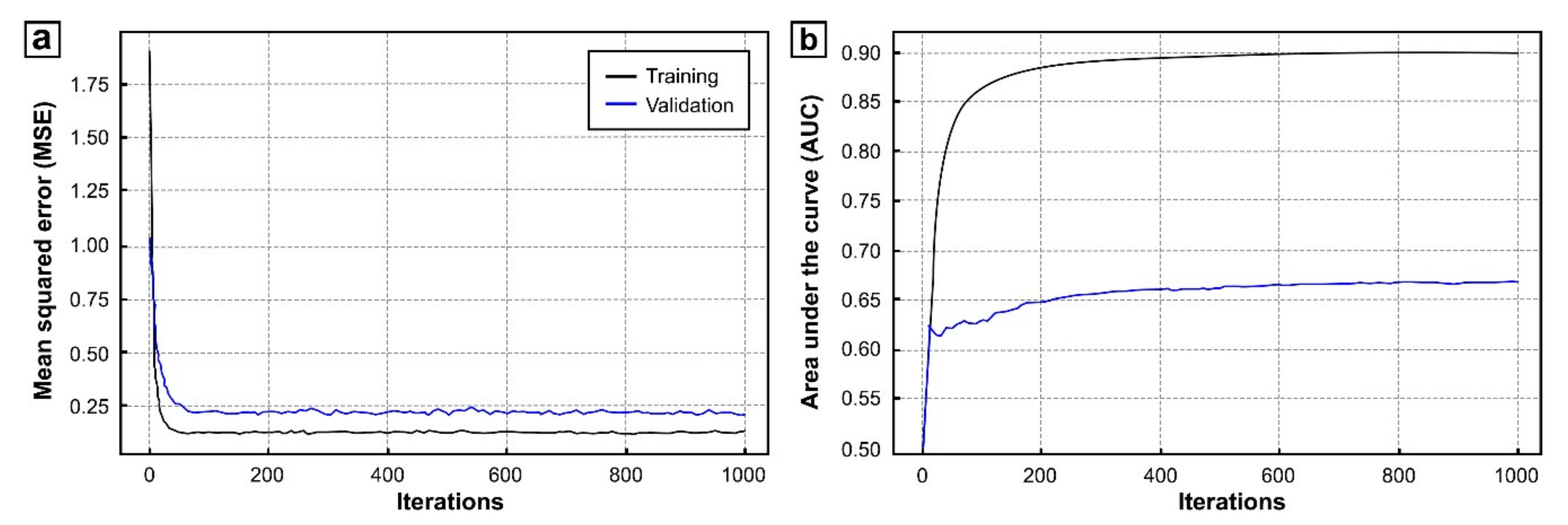
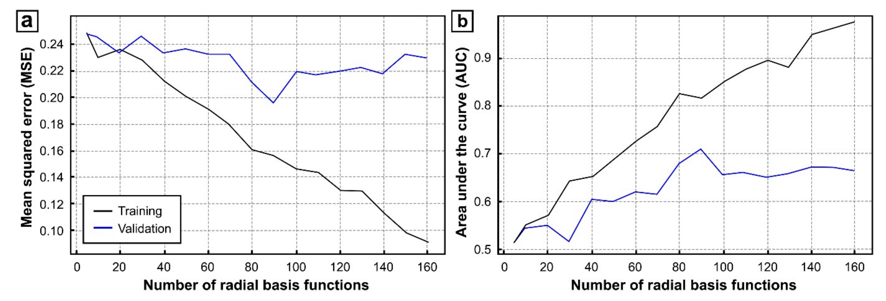
| Resolution | Phase | Iterations | Number of Hidden Neurons | Mean Squared Error (MSE) | Area under the Curve (AUC) |
|---|---|---|---|---|---|
| 500 m | training | 500 | 90 | 0.15 | 0.90 |
| validation | 0.20 | 0.65 | |||
| 250 m | training | 500 | 150 | 0.10 | 0.94 |
| validation | 0.22 | 0.63 |
© 2019 by the authors. Licensee MDPI, Basel, Switzerland. This article is an open access article distributed under the terms and conditions of the Creative Commons Attribution (CC BY) license (http://creativecommons.org/licenses/by/4.0/).
Share and Cite
Juliani, C.; Ellefmo, S.L. Prospectivity Mapping of Mineral Deposits in Northern Norway Using Radial Basis Function Neural Networks. Minerals 2019, 9, 131. https://doi.org/10.3390/min9020131
Juliani C, Ellefmo SL. Prospectivity Mapping of Mineral Deposits in Northern Norway Using Radial Basis Function Neural Networks. Minerals. 2019; 9(2):131. https://doi.org/10.3390/min9020131
Chicago/Turabian StyleJuliani, Cyril, and Steinar L. Ellefmo. 2019. "Prospectivity Mapping of Mineral Deposits in Northern Norway Using Radial Basis Function Neural Networks" Minerals 9, no. 2: 131. https://doi.org/10.3390/min9020131
APA StyleJuliani, C., & Ellefmo, S. L. (2019). Prospectivity Mapping of Mineral Deposits in Northern Norway Using Radial Basis Function Neural Networks. Minerals, 9(2), 131. https://doi.org/10.3390/min9020131