Stochastic Modeling of Chemical Compounds in a Limestone Deposit by Unlocking the Complexity in Bivariate Relationships


Abstract
1. Introduction
2. Methodology
2.1. Gaussian (Co)-Simulation
2.2. Projection Pursuit Multivariate Transform Steps
2.2.1. Preprocessing Steps
Normal Score Transformation
Data Sphering
Projection Pursuit
Stopping Criteria
Application
2.3. Proposed Algorithm
- Exploratory data analysis of multivariate data
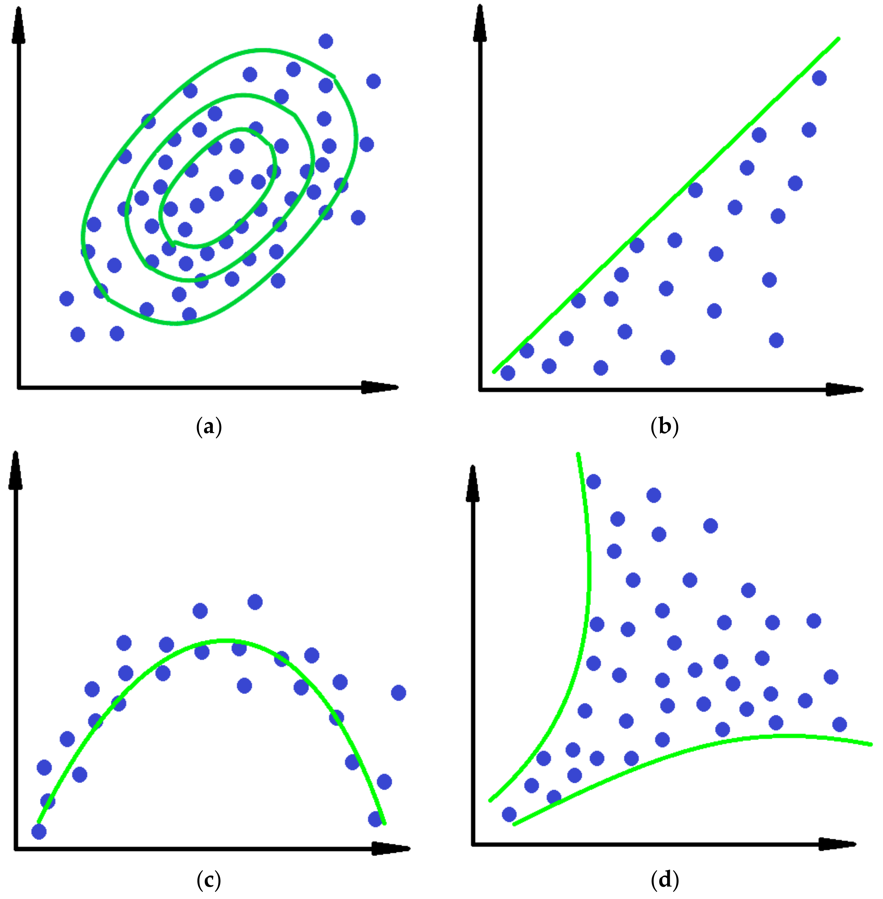
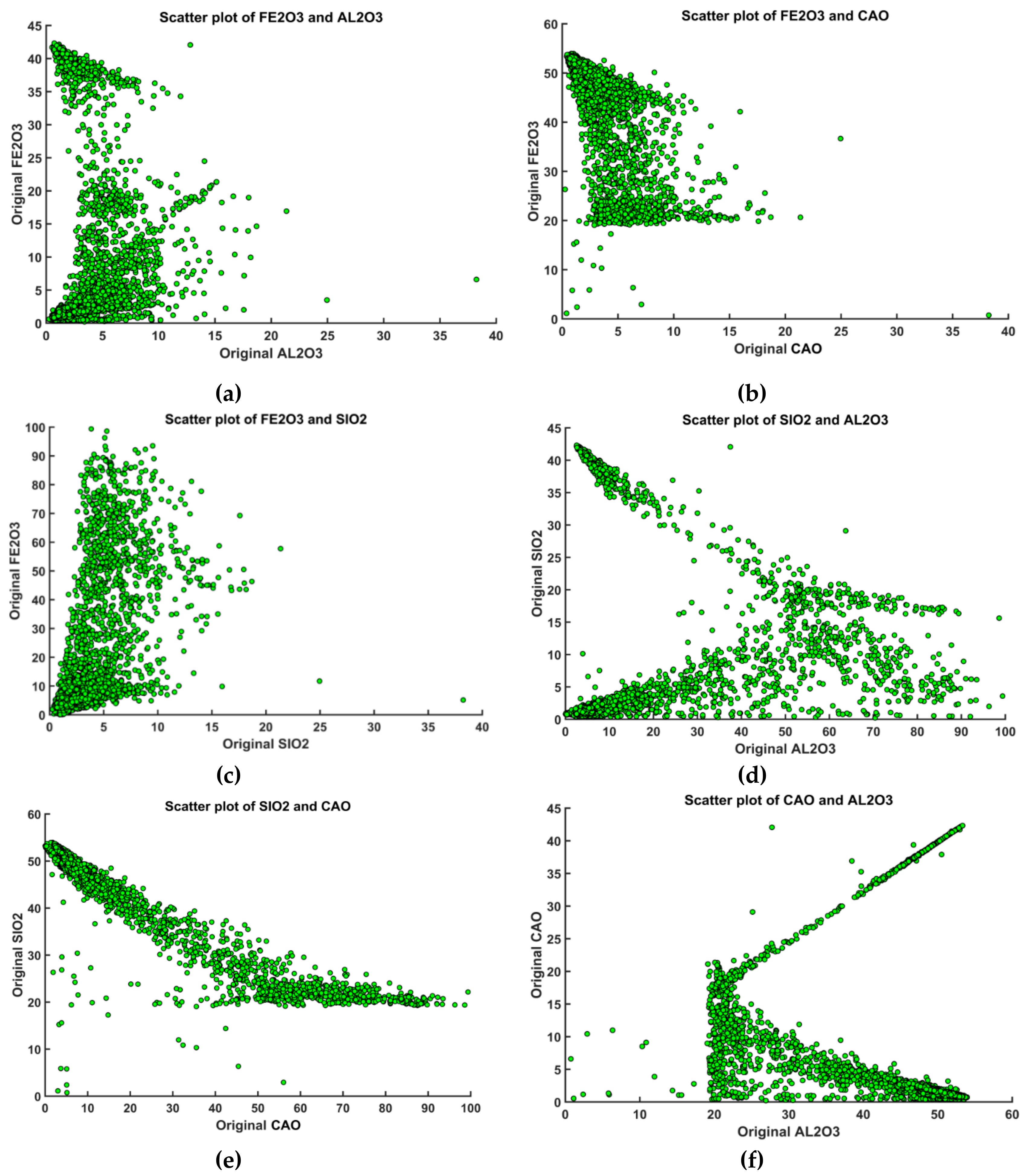
- Investigation of the level of complexity in bivariate relation analysis
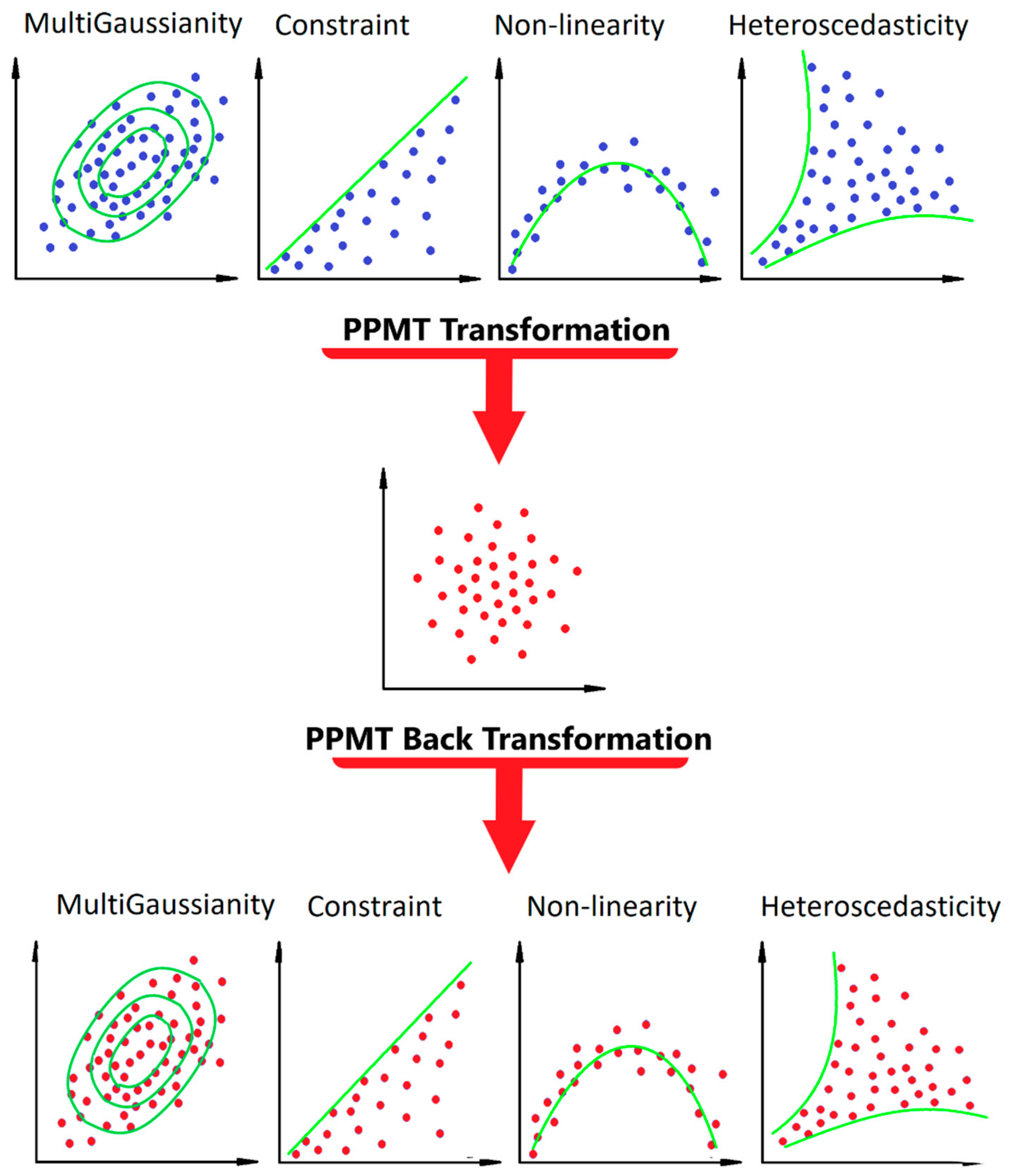
- PPMT forward transformation
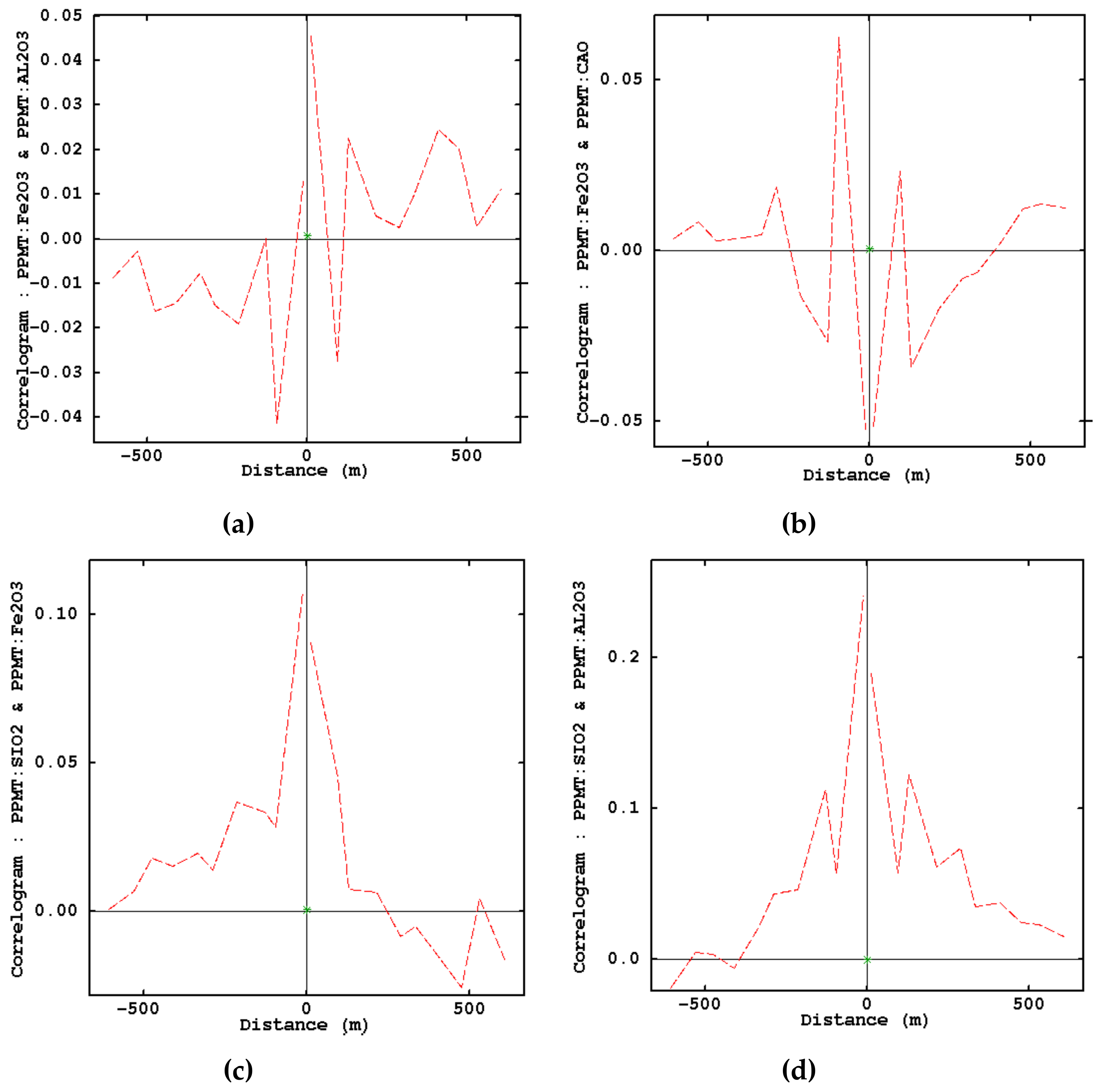
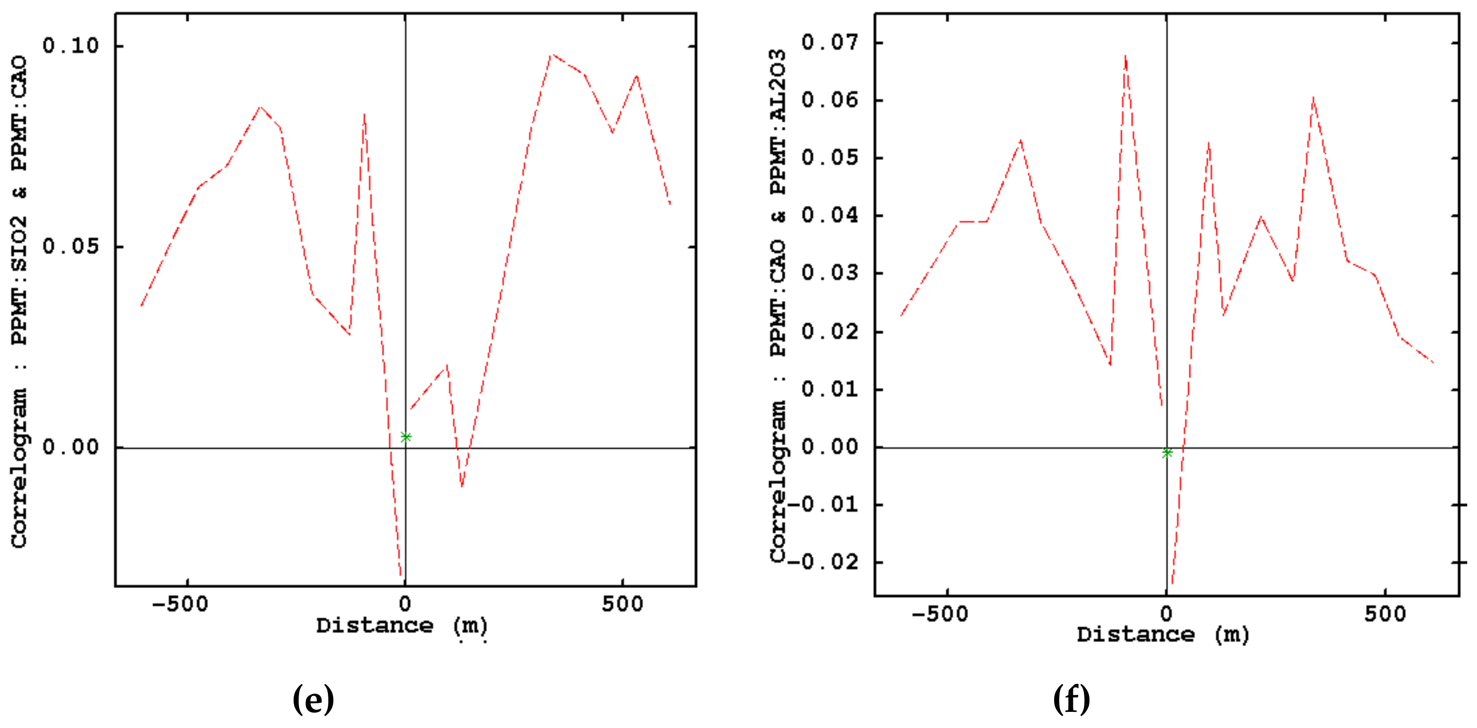
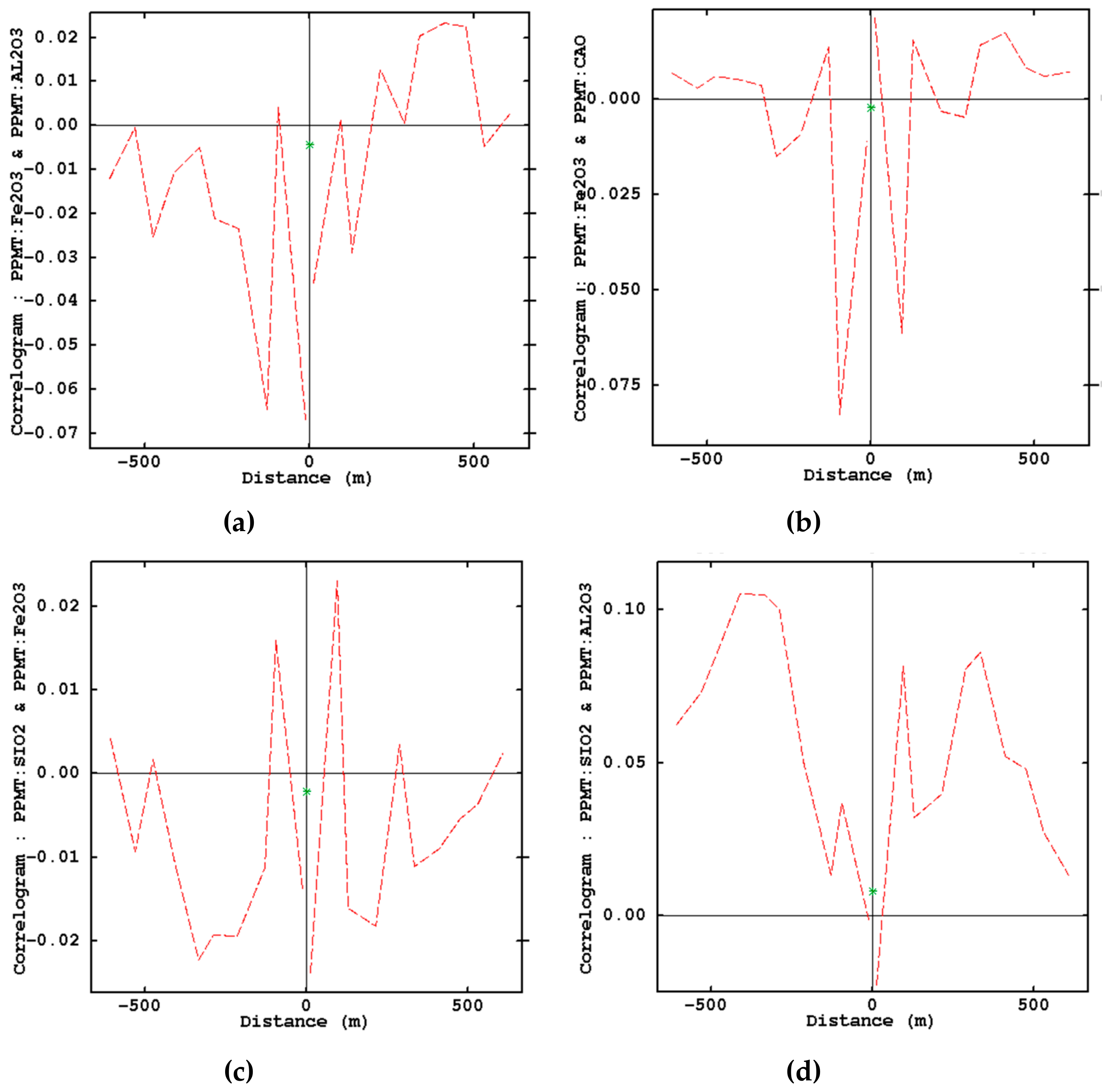
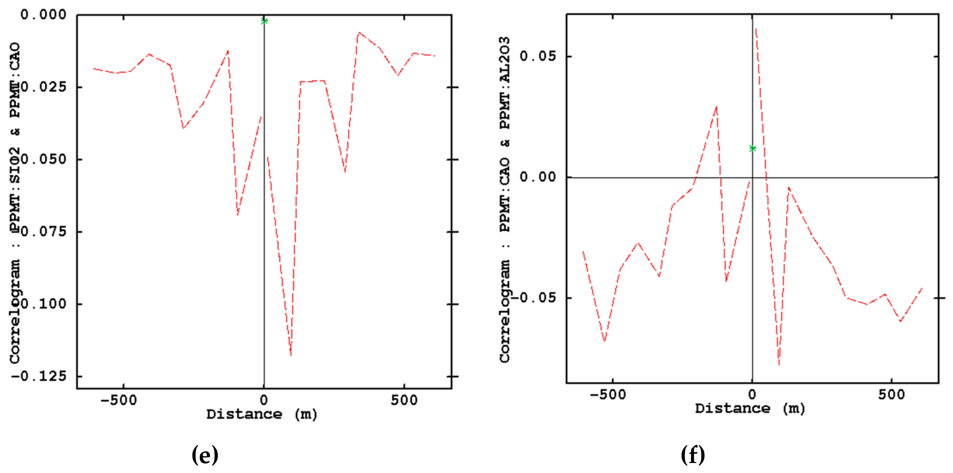
- Examination of removing cross-correlations among variables by using cross-correlogram
- Inference of cross-dependency functions by linear model of co-regionalization (LMC)
- (Co)-simulation of PPMT transformed factors taking into account the fitted LMC
- PPMT backward transformation of simulated results (realizations) into original scale
- Validation of the output by statistical analysis tools
3. Case Study: Aktas-South Deposit in Kazakhstan
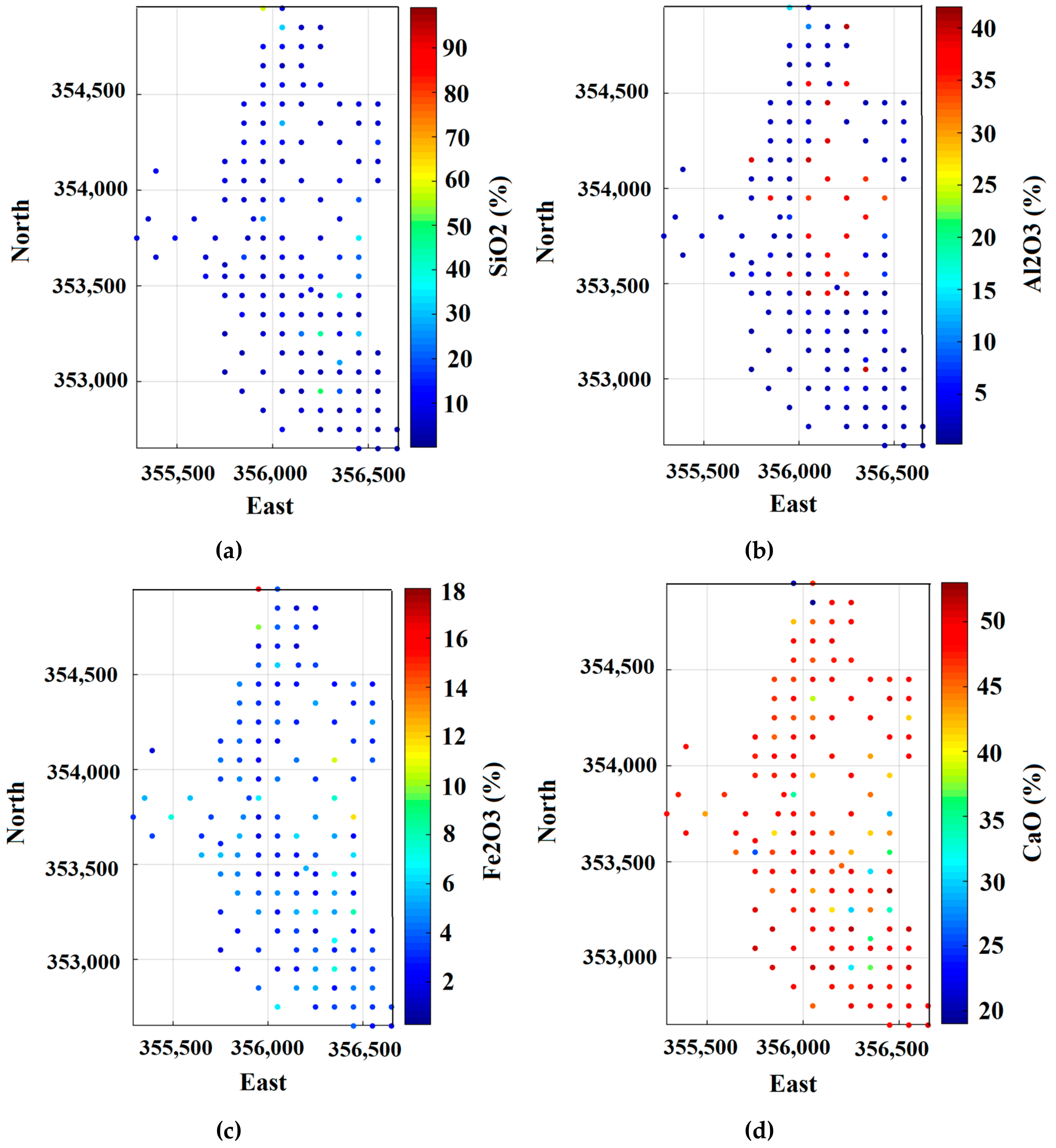
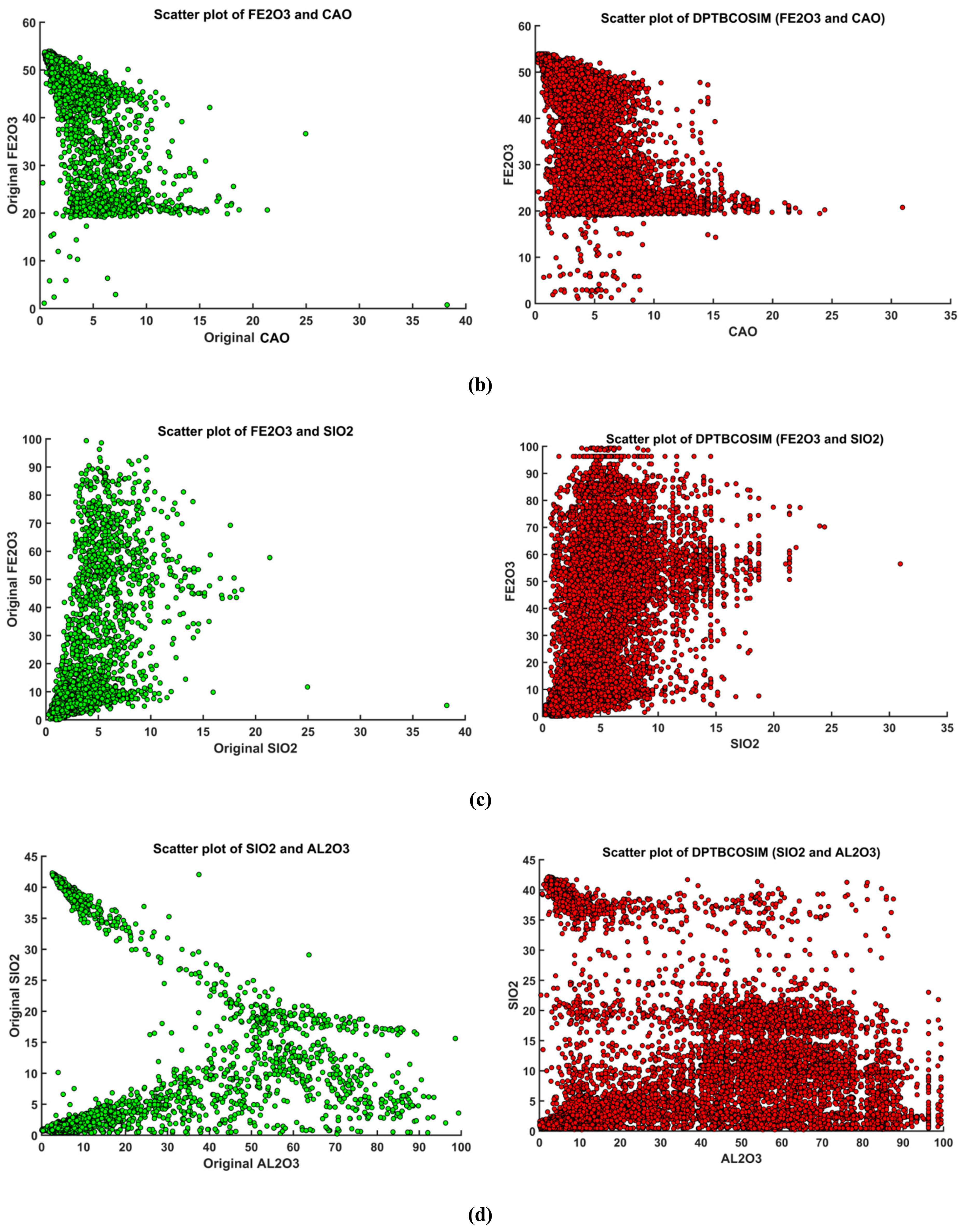
3.1. Exploratory Data Analysis in Limestone Deposit
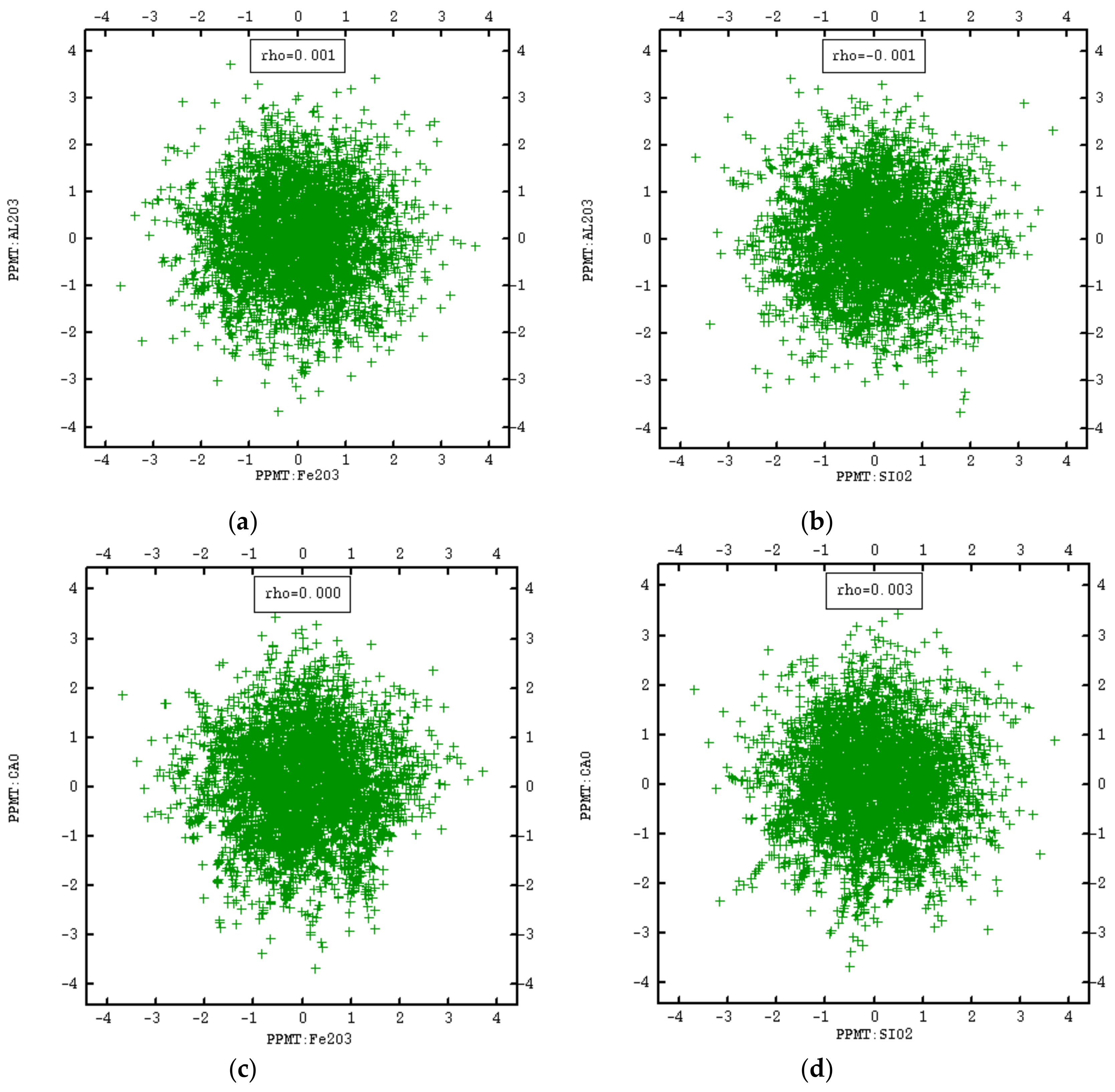
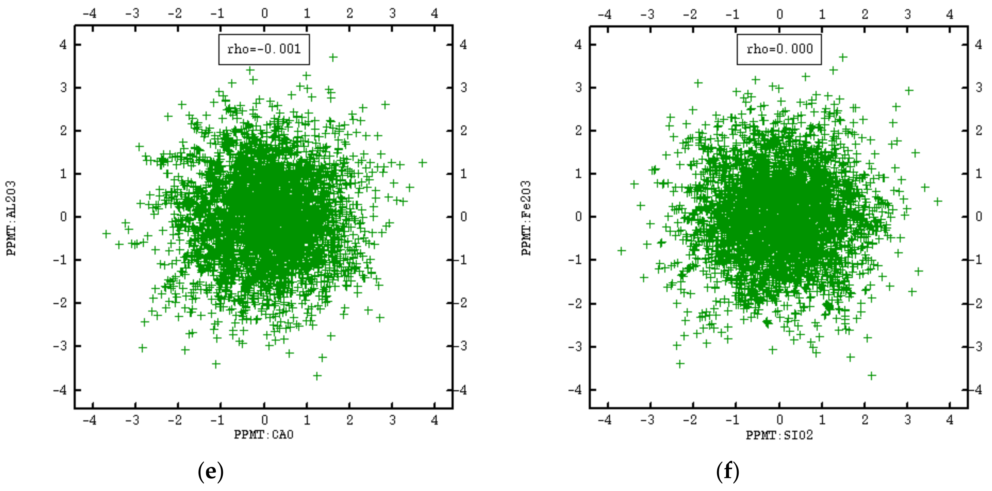
3.2. PPMT Forward Transformation
3.3. Variogram Inference
3.4. Stochastic Modeling in Limestone Deposit
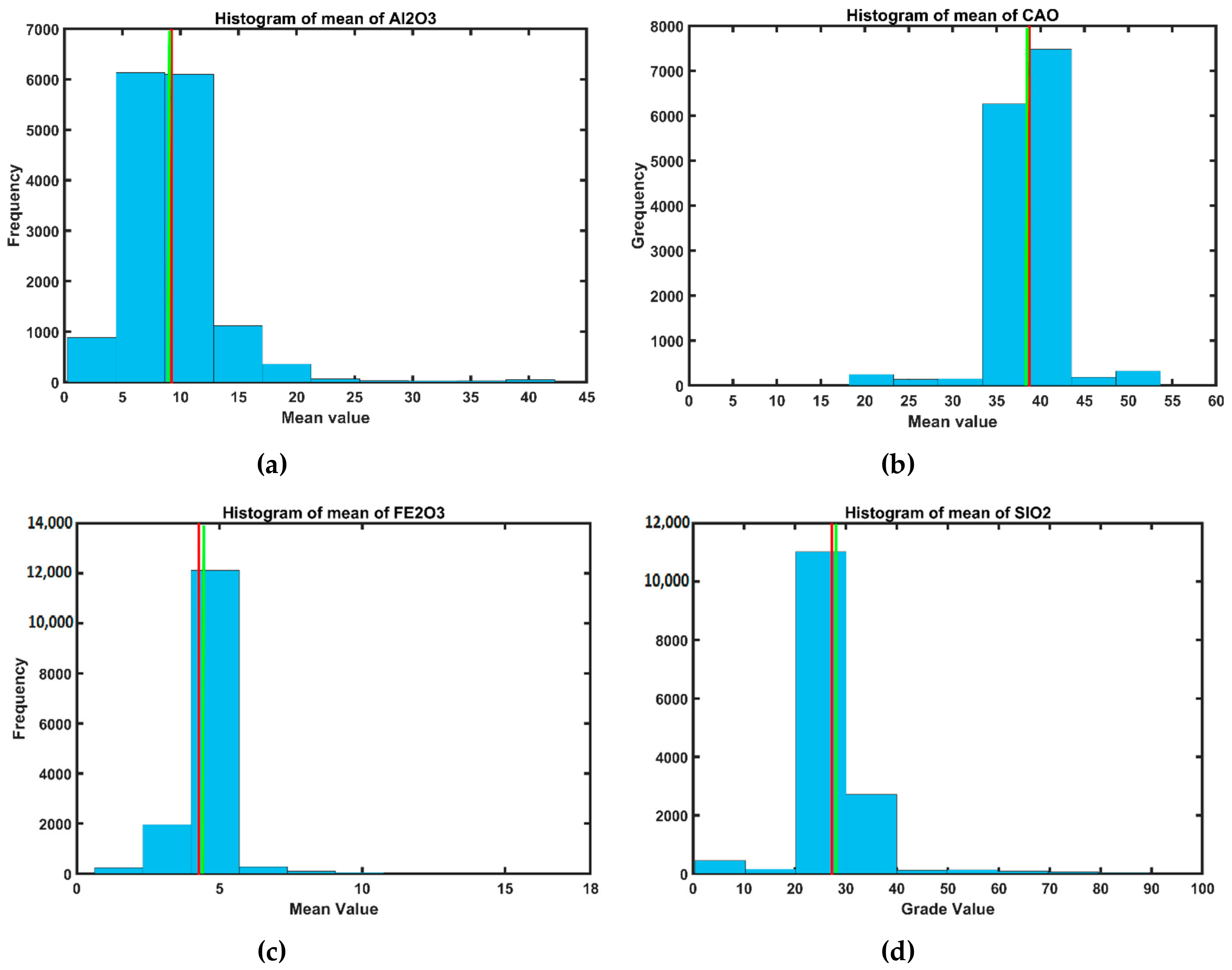
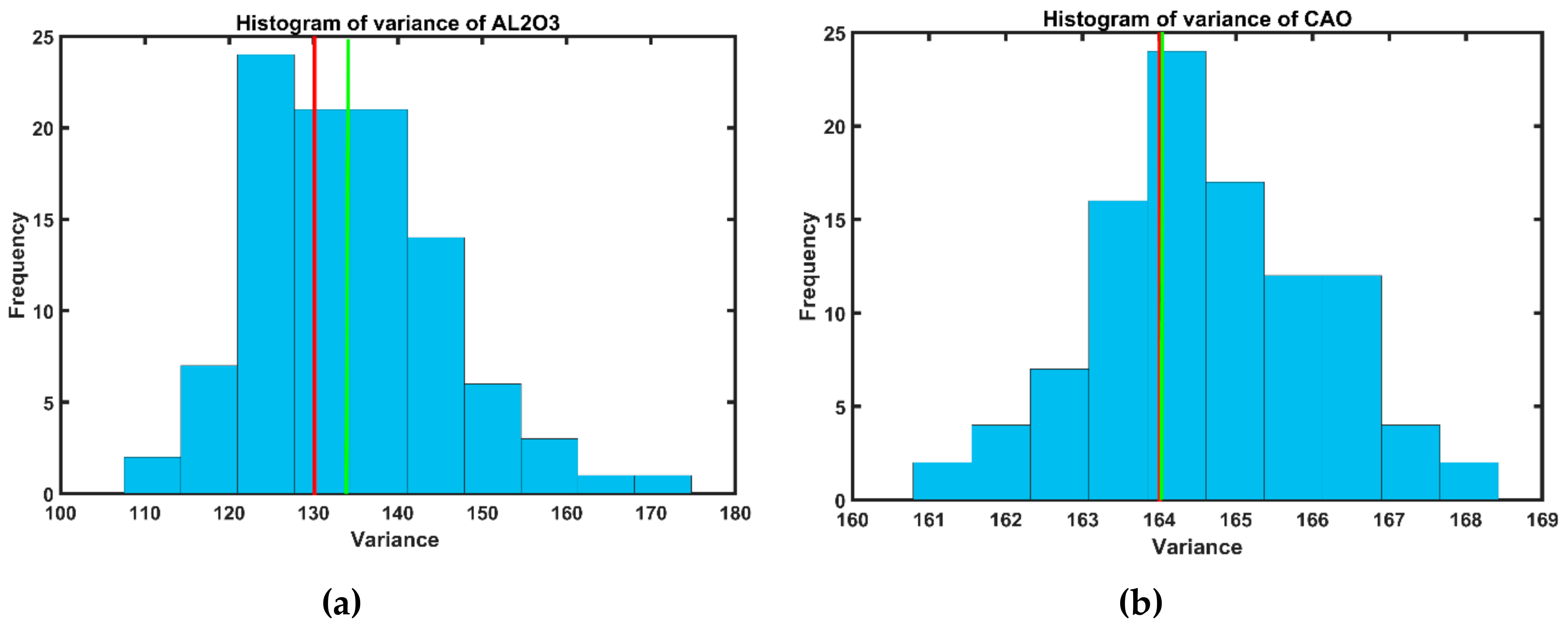
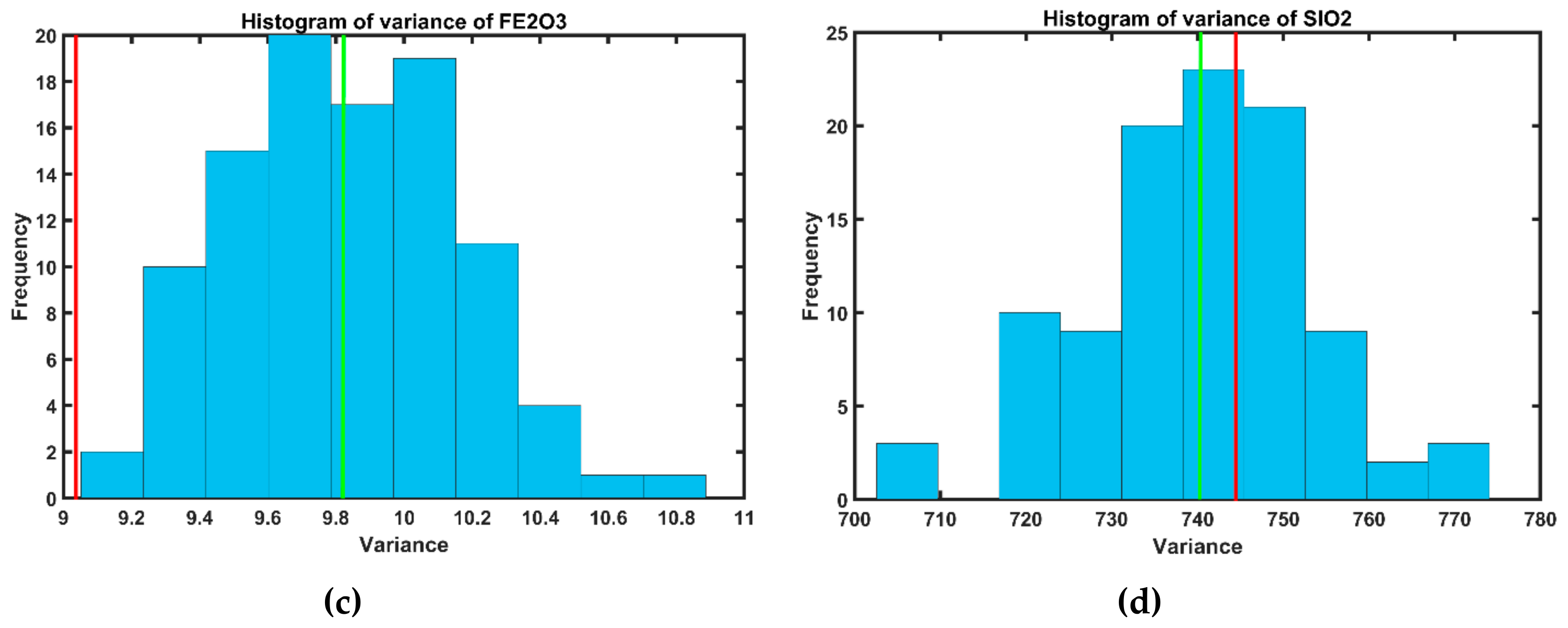
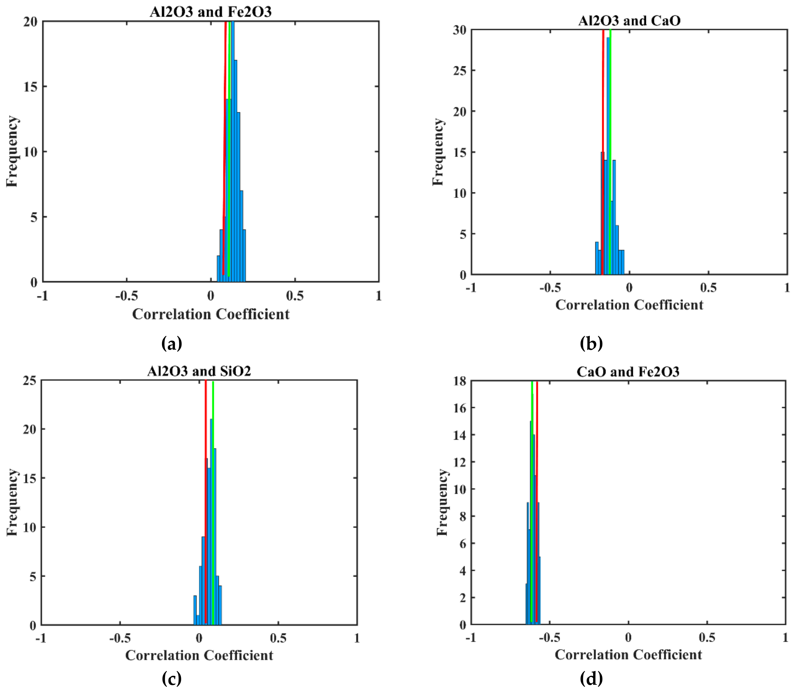
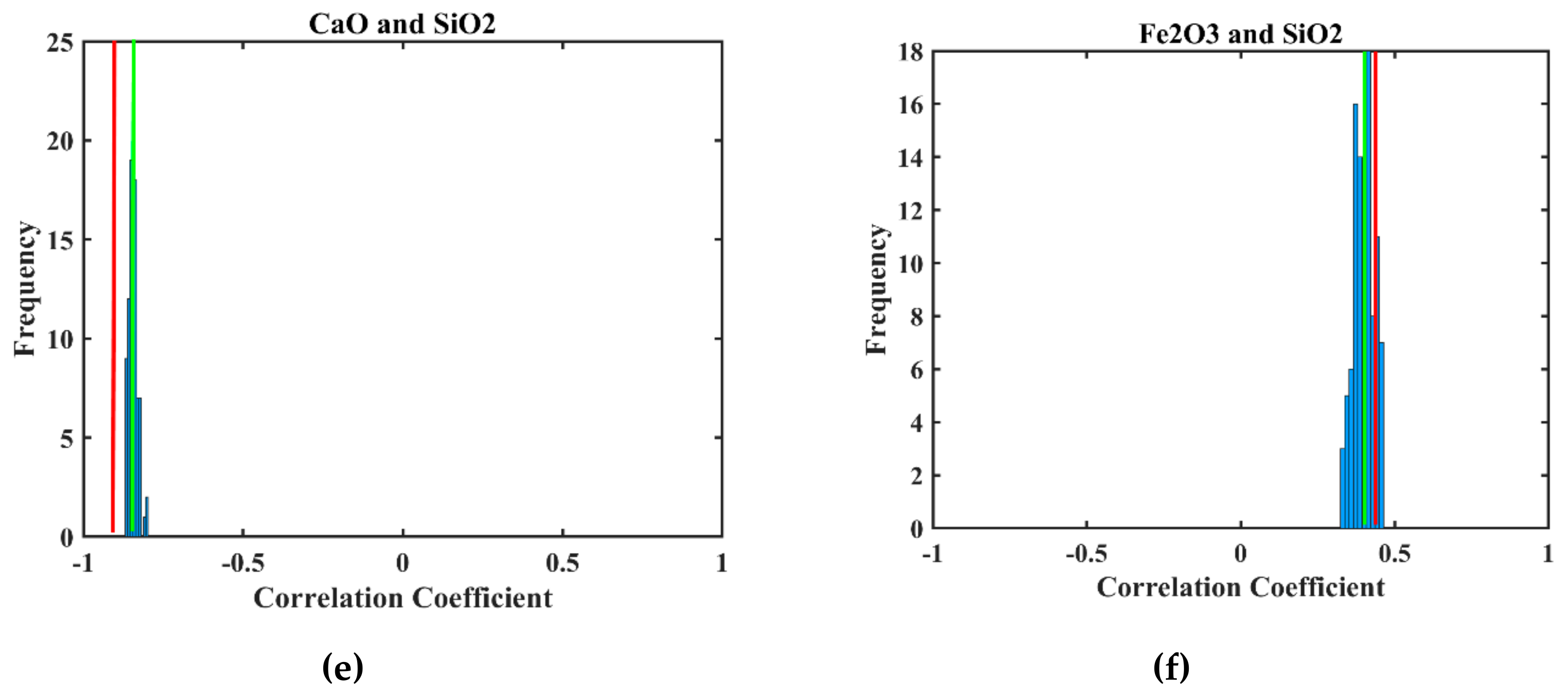
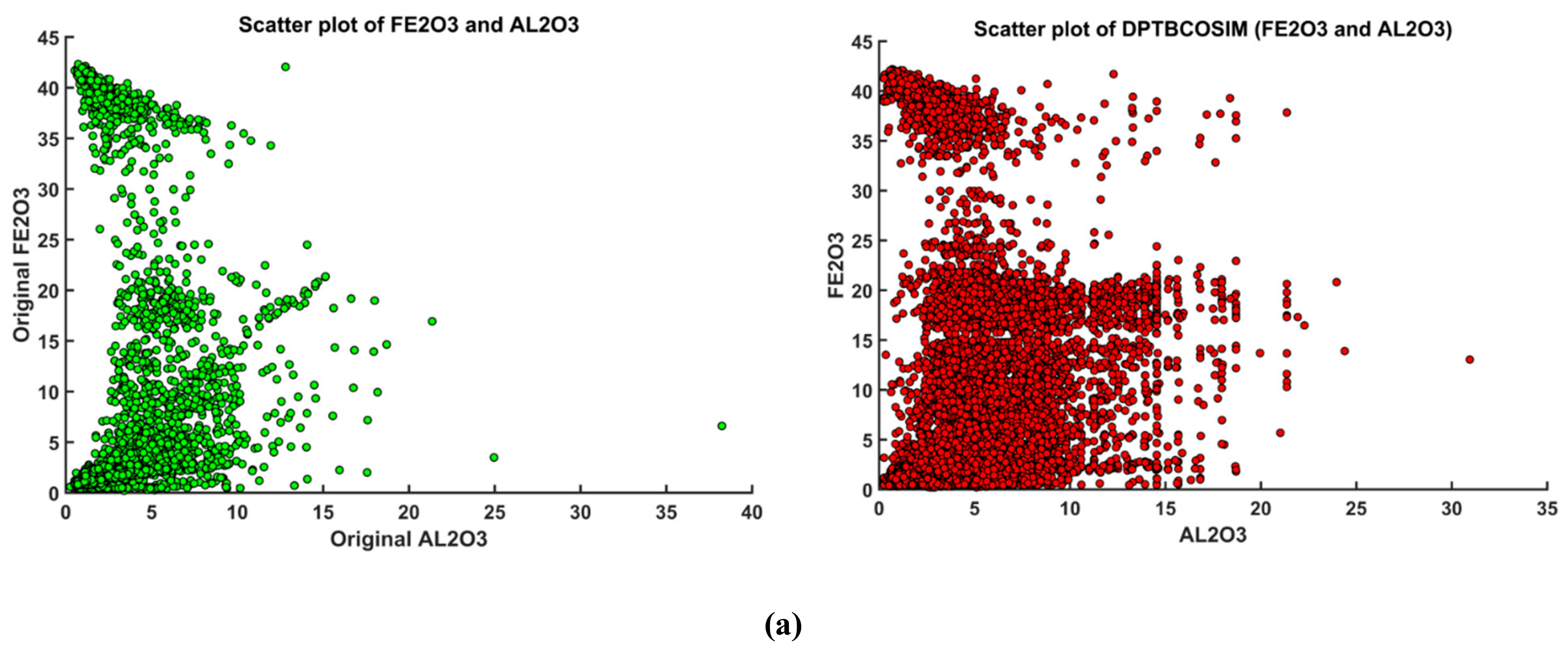
3.5. Validation
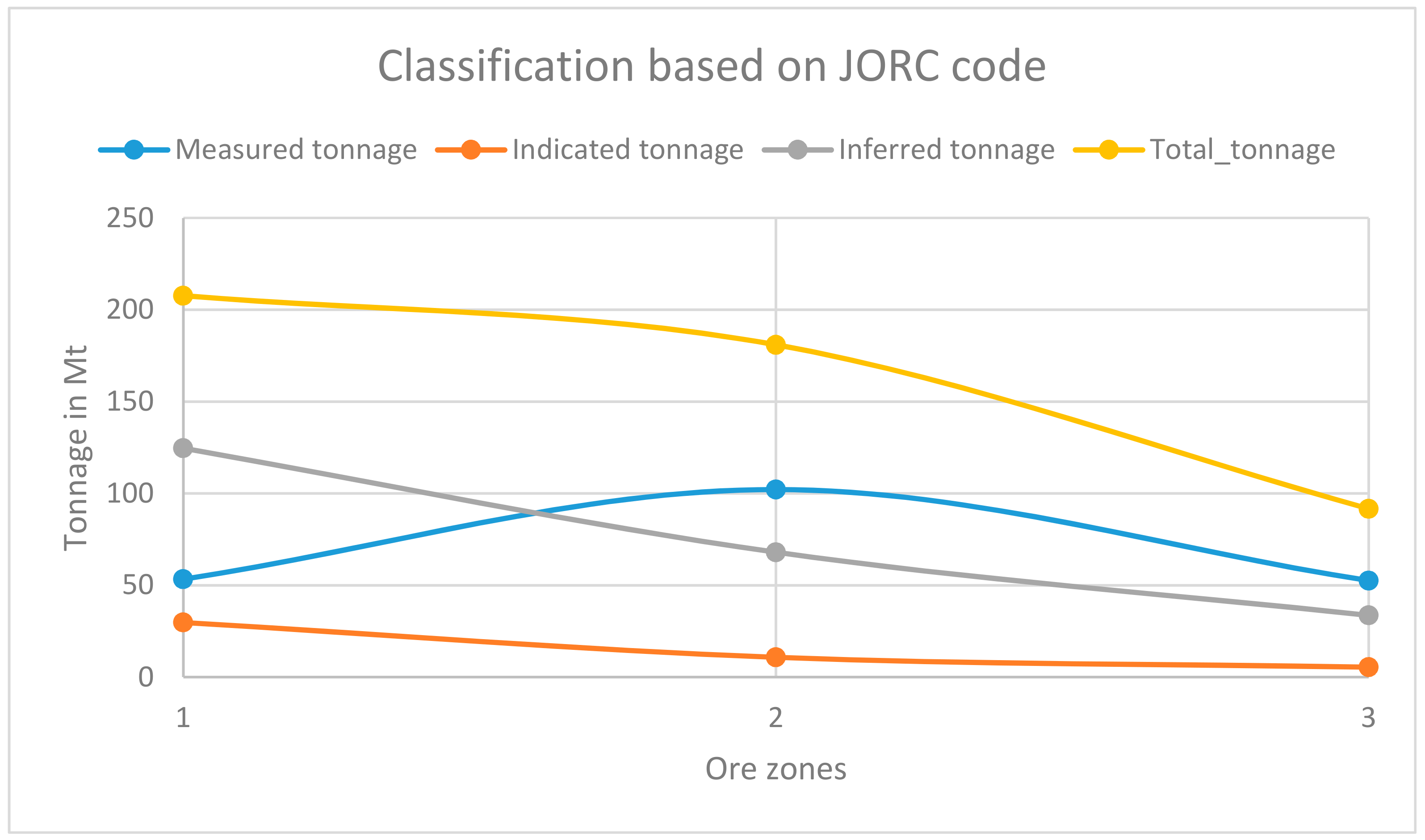
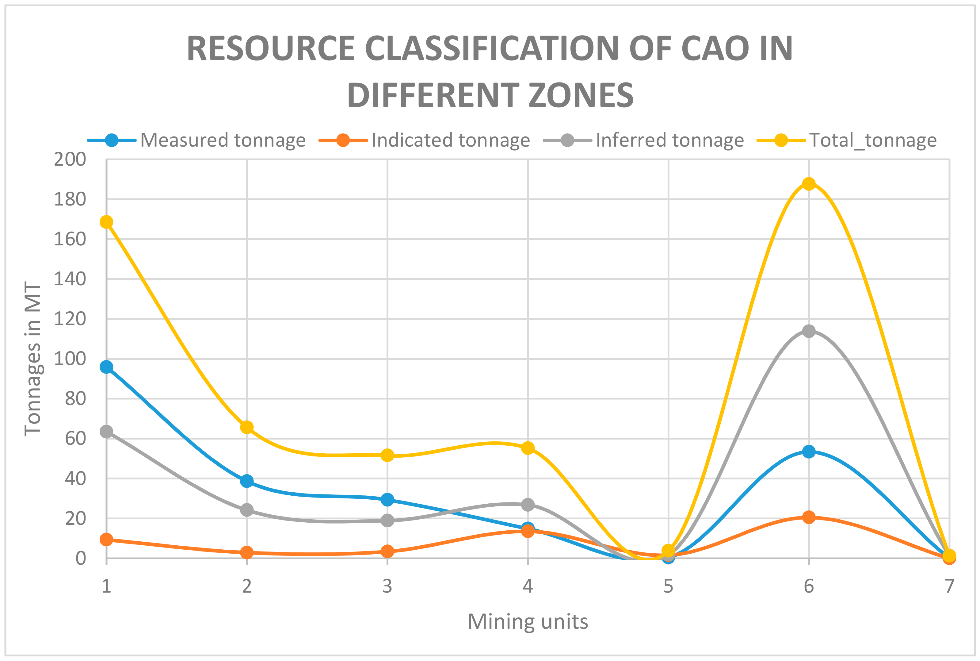
3.6. Mineral Resource Classification
3.6.1. Ore Zone Definitions
3.6.2. Mining Units
4. Conclusions
Author Contributions
Funding
Acknowledgments
Conflicts of Interest
References
- Dimitrakopoulos, R. Stochastic Mine Planning—Methods, Examples and Value in an Uncertain World. In Advances in Applied Strategic Mine Planning; Springer: Cham, Switzerland, 2018; pp. 101–115. [Google Scholar]
- Hustrulid, W.A.; Kuchta, M.; Martin, R.K. Open Pit Mine Planning and Design, Two Volume Set & CD-ROM Pack: V1: Fundamentals, V2: CSMine Software Package, CD-ROM: CS Mine Software; CRC Press: Boca Raton, FL, USA, 2013. [Google Scholar]
- Kasmaee, S.; Raspa, G.; De Fouquet, C.; Tinti, F.; Bonduà, S.; Bruno, R. Geostatistical Estimation of Multi-Domain Deposits with Transitional Boundaries: A Sensitivity Study for the Sechahun Iron Mine. Minerals 2019, 9, 115. [Google Scholar] [CrossRef]
- Joint Ore Reserves Committee (JORC) Code. The JORC Code and Guidelines. In Australasian Code for Reporting of Exploration Results, Mineral Resources and Ore Reserves Prepared by The Australasian Institute of Mining and Metallurgy (AusIMM); Australian Institute of Geoscientists and Minerals Council of Australia: Crows Nest, Australia, 2012; Available online: www.jorc.org (accessed on 7 October 2015).
- Monkhouse, P.H.L.; Yeates, G.A. Beyond Naive Optimisation. In Advances in Applied Strategic Mine Planning; Springer: Cham, Switzerland, 2018; pp. 3–18. [Google Scholar]
- Mai, N.L.; Erten, O.; Topal, E. A new generic open pit mine planning process with risk assessment ability. Int. J. Coal Sci. Technol. 2016, 3, 407–417. [Google Scholar] [CrossRef]
- Dimitrakopoulos, R. Stochastic optimization for strategic mine planning: A decade of developments. J. Min. Sci. 2011, 47, 138–150. [Google Scholar] [CrossRef]
- Khosrowshahi, S.; Shaw, W.J.; Yeates, G.A. Quantification of Risk Using Simulation of the Chain of Mining—Case Study at Escondida Copper, Chile. In Advances in Applied Strategic Mine Planning; Springer: Cham, Switzerland, 2018; pp. 57–74. [Google Scholar]
- Vallejo, M.N.; Dimitrakopoulos, R. Stochastic orebody modelling and stochastic long-term production scheduling at the KéMag iron ore deposit, Quebec, Canada. Int. J. Mining Reclam. Environ. 2018, 33, 462–479. [Google Scholar] [CrossRef]
- Benndorf, J.; Dimitrakopoulos, R. Stochastic long-term production scheduling of iron ore deposits: Integrating joint multi-element geological uncertainty. J. Min. Sci. 2013, 49, 68–81. [Google Scholar] [CrossRef]
- De-Vitry, C.; Vann, J.; Arvidson, H. Multivariate iron ore deposit resource estimation—A practitioner’s guide to selecting methods. Appl. Earth Sci. 2010, 119, 154–165. [Google Scholar] [CrossRef]
- Dimitrakopoulos, R.; Farrelly, C.T.; Godoy, M. Moving forward from traditional optimization: Grade uncertainty and risk effects in open-pit design. Min. Technol. 2002, 111, 82–88. [Google Scholar] [CrossRef]
- Menabde, M.; Froyland, G.; Stone, P.; Yeates, G.A. Mining Schedule Optimisation for Conditionally Simulated Orebodies. In Advances in Applied Strategic Mine Planning; Springer: Cham, Switzerland, 2018; pp. 91–100. [Google Scholar]
- Dimitrakopoulos, R. Conditional simulation algorithms for modelling orebody uncertainty in open pit optimisation. Int. J. Surf. Min. Reclam. Environ. 1998, 12, 173–179. [Google Scholar] [CrossRef]
- Emery, X.; Lantue´joul, C. Tbsim: A computer program for conditional simulation of three-dimensional gaussian random fields via the turning bands method. Comput. Geosci. 2006, 32, 1615–1628. [Google Scholar] [CrossRef]
- Isaaks, E.H. The Application of Monte Carlo Methods to the Analysis of Spatially Correlated Data: Unpublished. Ph.D. Thesis, Stanford University, Stanford, CA, USA, 1999; 213p. [Google Scholar]
- Journel, A.G. Modeling Uncertainty: Some Conceptual Thoughts. In Geostatistics Valencia 2016; Springer: Cham, Switzerland, 1994; Volume 6, pp. 30–43. [Google Scholar]
- Boisvert, J.B.; Rossi, M.E.; Ehrig, K.; Deutsch, C.V. Geometallurgical Modeling at Olympic Dam Mine, South Australia. Math. Geosci. 2013, 45, 901–925. [Google Scholar] [CrossRef]
- Deutsch, C.V. Geostatistical Modelling of Geometallurgical Variables–Problems and Solutions. In Proceedings of the Second AUSIMM International Geometallurgy Conference/Brisbane, Brisbane, Australia, 30 September 2013; Volume 30, pp. 7–15. [Google Scholar]
- Leuangthong, O.; Deutsch, C.V. Stepwise Conditional Transformation for Simulation of Multiple Variables. Math. Geosci. 2003, 35, 155–173. [Google Scholar]
- Van den Boogaart, K.G.; Mueller, U.; Tolosana-Delgado, R. An affine equivariant multivariate normal score transform for compositional data. Math. Geosci. 2017, 49, 231–251. [Google Scholar] [CrossRef]
- Barnett, R.; Manchuk, J.; Deutsch, C. Projection pursuit multivariate transform. Math. Geosci. 2014, 46, 337–359. [Google Scholar] [CrossRef]
- Barnett, R.M.; Manchuk, J.G.; Deutsch, C.V. The Projection-Pursuit Multivariate Transform for Improved Continuous Variable Modeling. SPE J. 2016, 21, 2010–2026. [Google Scholar] [CrossRef]
- Battalgazy, N.; Madani, N. Categorization of Mineral Resources Based on Different Geostatistical Simulation Algorithms: A Case Study from an Iron Ore Deposit. Nat. Resour. Res. 2019, 28, 1329–1351. [Google Scholar] [CrossRef]
- Adeli, A.; Emery, X.; Dowd, P. Geological Modelling and Validation of Geological Interpretations via Simulation and Classification of Quantitative Covariates. Minerals 2017, 8, 7. [Google Scholar] [CrossRef]
- Shao, H.; Sun, X.; Wang, H.; Zhang, X.; Xiang, Z.; Tan, R.; Chen, X.; Xian, W.; Qi, J. A method to the impact assessment of the returning grazing land to grassland project on regional eco-environmental vulnerability. Environ. Impact Assess. Rev. 2017, 56, 155–167. [Google Scholar] [CrossRef]
- Vasylchuk, Y.V.; Deutsch, C.V. Improved grade control in open pit mines. Min. Technol. 2018, 127, 84–91. [Google Scholar] [CrossRef]
- Rivoirard, J. Introduction to Disjunctive Kriging and Non-Linear Geostatistics; Clarendon Press: Oxford, UK, 1994; 181p. [Google Scholar]
- Deutsch, C.V.; Journel, A.G. GSLIB: Geostatistical Software Library and User’s Guide, 2nd ed.; Oxford University Press: New York, NY, USA, 1998. [Google Scholar]
- Journel, A.G.; Huijbregts, C.J. Mining Geostatistics; Academic Press: London, UK, 1978. [Google Scholar]
- Barnett, R.M. Projection Pursuit Multivariate Transform. In Geostatistics Lessons; Deutsch, J.L., Ed.; Centre for Computational Geostatistics, Department of Civil and Environmental Engineering, University of Alberta: Edmonton, AB, Canada, 2017; Available online: http://www.geostatisticslessons.com/lessons/lineardecorrelation.html (accessed on 24 October 2018).
- Reed, M.; Simon, B. Methods of Modern Mathematical Physics. I, II, III, IV; Academic Press Inc.: New York, NY, USA, 1972; Volume 1975, p. 1979. [Google Scholar]
- Emery, X. A turning bands program for conditional co-simulation of cross-correlated Gaussian random fields. Comput. Geosci. 2008, 34, 1850–1862. [Google Scholar] [CrossRef]
- Verly, G.W. Sequential Gaussian Cosimulation: A Simulation Method Integrating Several Types of Information. In Geostatistics Valencia 2016; Springer: Cham, Switzerland, 1993; Volume 5, pp. 543–554. [Google Scholar]
- Abildin, Y.; Madani, N.; Topal, E. A Hybrid Approach for Joint Simulation of Geometallurgical Variables with Inequality Constraint. Minerals 2019, 9, 24. [Google Scholar] [CrossRef]
- Wackernagel, H. Multivariate Geostatistics: An Introduction with Applications; Springer: Berlin/Heidelberg, Germany, 2003. [Google Scholar]
- Rivoirard, J.; Demange, C.; Freulon, X.; Lécureuil, A.; Bellot, N. A top-cut model for deposits with heavy-tailed grade distribution. Math. Geosci. 2013, 45, 967–982. [Google Scholar] [CrossRef]
- Maleki, M.; Madani, N.; Emery, X. Capping and kriging grades with long-tailed distributions. J. South. Afr. Inst. Min. Metall. 2014, 114, 255–263. [Google Scholar]
- Sinclair, A.J.; Blackwell, G.H. Applied Mineral Inventory Estimation; Cambridge University Press (CUP): Cambridge, UK, 2002. [Google Scholar]
- Deutsch, J.L.; Deutsch, C.V. Some Geostatistical Software Implementation Details; Centre for Computational Geostatistics, University of Alberta: Edmonton, AB, Canada, 2010; Volume 412. [Google Scholar]
- Rossi, M.E.; Deutsch, C.V. Mineral Resource Estimation; Springer: Berlin, Germany, 2014. [Google Scholar]
- Madani, N.; Yagiz, S.; Adoko, A.C. Spatial Mapping of the Rock Quality Designation Using Multi-Gaussian Kriging Method. Minerals 2018, 8, 530. [Google Scholar] [CrossRef]
- Goovaerts, P. Geostatistics for Natural Resources Evaluation; Oxford University Press: New York, NY, USA, 1997. [Google Scholar]
- Leuangthong, O.; Khan, K.D.; Deutsch, C.V. Solved Problems in Geostatistics; John Wiley & Sons: Hoboken, NJ, USA, 2011. [Google Scholar]
- Emery, X. Iterative algorithms for fitting a linear model of coregionalization. Comput. Geosci. 2010, 36, 1150–1160. [Google Scholar] [CrossRef]
- Maleki, M.; Emery, X.; Mery, N. Indicator Variograms as an Aid for Geological Interpretation and Modeling of Ore Deposits. Minerals 2017, 7, 241. [Google Scholar] [CrossRef]
- Paravarzar, S.; Emery, X.; Madani, N. Comparing sequential Gaussian simulation and turning bands algorithms for cosimulating grades in multi-element deposits. Comptes Rendus Geosci. 2015, 347, 84–93. [Google Scholar] [CrossRef]
- Madani, N.; Emery, X. A comparison of search strategies to design the cokriging neighborhood for predicting coregionalized variables. Stoch. Environ. Res. Risk Assess. 2019, 33, 183–199. [Google Scholar] [CrossRef]
- Lantue´joul, C. Geostatistical Simulation, Models and Algorithms; Springer: Berlin, Germany, 2002. [Google Scholar]
- Madani, N.; Carranza, E.J.M. Co-simulated Size Number: An Elegant Novel Algorithm for Identification of Multivariate Geochemical Anomalies. Nat. Resour. Res. 2019, in press. [Google Scholar] [CrossRef]
- Eze, P.N.; Madani, N.; Adoko, A.C. Multivariate mapping of heavy metals spatial contamination in a Cu–Ni exploration field (Botswana) using turning bands co-simulation algorithm. Nat. Resour. Res. 2019, 28, 109–124. [Google Scholar] [CrossRef]
- Madani, N. Multi-collocated cokriging: An application to grade estimation in the mining industry. In Mining Goes Digital; CRC Press: Wroclaw, Poland, 2019; pp. 158–167. [Google Scholar]
- Maleki, M.; Madani, N. Multivariate geostatistical analysis: An application to ore body evaluation. Iranian J. Earth Sci. 2017, 8, 173–184. [Google Scholar]


| Lithology | Physical Appearance | Chemical Characteristics | Comment |
|---|---|---|---|
| Cherty limestone (CL) | Yellow in color with alternating cherty bands | Not ascertained | Likely to be used in cement after removing cherty bands |
| Pale yellow limestone (PYLS) | Yellow to pale brown in color | >40% CaO and <3.5% Fe2O3 | Very good for cement manufacturing |
| Brown cherty limestone (BCLS) | Brown to dark brown | >8% Fe2O3 | |
| Ferruginous limestone (FLS) | Brown to dark brown | >40% CaO and Fe2O3 > 3.5% to 10 | Considered as low grade limestone |
| Variable (%) | Number of Samples | Minimum | Maximum | Mean | Variance | Coefficient of Variation (COV) |
|---|---|---|---|---|---|---|
| Al2O3 | 4553 | 0.21 | 42.32 | 9.33 | 132.92 | 1.23 |
| CaO | 4553 | 0.75 | 53.94 | 38.79 | 164.14 | 0.33 |
| Fe2O3 | 4553 | 0.26 | 38.24 | 4.29 | 9.04 | 0.70 |
| SiO2 | 4553 | 0.03 | 99.37 | 27.24 | 744.72 | 1.00 |
| Variables | Fe2O3 | Al2O3 | CaO | SiO2 |
|---|---|---|---|---|
| Fe2O3 | 1 | 0.13 | −0.64 | 0.53 |
| Al2O3 | 1 | −0.17 | 0.13 | |
| CaO | 1 | −0.94 | ||
| SiO2 | 1 |
| Zone | Chemical Cutoffs |
|---|---|
| Marl-chert | ≤40% and ≥20% of CaO |
| Pale yellow limestone | >40% of CaO and <3% of Fe2O3 |
| Brown limestone | >40% of CaO and ≥3% and <4.5% of Fe2O3 |
| Classification | Marl-Chert (Mt) | Pale Yellow Limestone (Mt) | Brown Limestone (Mt) |
|---|---|---|---|
| Measured | 53 | 102.14288 | 52.56608 |
| Indicated | 30 | 10.79 | 5.4357 |
| Inferred | 125 | 67.99632 | 33.652 |
| Total | 208 | 180.9292 | 91.65378 |
| Mining Unit | Chemical Cutoffs |
|---|---|
| HGLS | CaO ≥ 40 and SiO2 ≤15 and Fe2O3 < 3 |
| BROWNLS | CaO ≥ 40 and SiO2 ≤ 15 and Fe2O3 ≥ 3 and Fe2O3 < 4 |
| FEROLS | CaO ≥ 40 and SiO2 ≤ 15 and Fe2O3 ≥ 4 |
| CHERTYLS | CaO < 50 and CaO > 20 and SiO2 > 15 and SiO2 ≤40 |
| CHERTYLS2 | CaO < 40 and CaO > 30 and SiO2 ≤15 |
| MARL | CaO < 45 and CaO > 10 and SiO2 > 40 |
| WASTE | CaO ≤ 10 and CaO > 0 and SiO2 > 40 |
| Category | HGLS | BROWNLS | FEROLS | CHERTYLS | CHERTYLS2 | MARL | WASTE |
|---|---|---|---|---|---|---|---|
| Measured tonnage | 95.8 | 38.6 | 29.3 | 14.9 | 0.4 | 53.4 | 0.0 |
| Indicated tonnage | 9.3 | 2.8 | 3.4 | 13.5 | 1.5 | 20.4 | 0.0 |
| Inferred tonnage | 63.4 | 24.1 | 18.9 | 26.8 | 1.8 | 113.8 | 1.2 |
| Total tonnage | 168.5 | 65.6 | 51.5 | 55.1 | 3.7 | 187.5 | 1.2 |
© 2019 by the authors. Licensee MDPI, Basel, Switzerland. This article is an open access article distributed under the terms and conditions of the Creative Commons Attribution (CC BY) license (http://creativecommons.org/licenses/by/4.0/).
Share and Cite
Battalgazy, N.; Madani, N. Stochastic Modeling of Chemical Compounds in a Limestone Deposit by Unlocking the Complexity in Bivariate Relationships. Minerals 2019, 9, 683. https://doi.org/10.3390/min9110683
Battalgazy N, Madani N. Stochastic Modeling of Chemical Compounds in a Limestone Deposit by Unlocking the Complexity in Bivariate Relationships. Minerals. 2019; 9(11):683. https://doi.org/10.3390/min9110683
Chicago/Turabian StyleBattalgazy, Nurassyl, and Nasser Madani. 2019. "Stochastic Modeling of Chemical Compounds in a Limestone Deposit by Unlocking the Complexity in Bivariate Relationships" Minerals 9, no. 11: 683. https://doi.org/10.3390/min9110683
APA StyleBattalgazy, N., & Madani, N. (2019). Stochastic Modeling of Chemical Compounds in a Limestone Deposit by Unlocking the Complexity in Bivariate Relationships. Minerals, 9(11), 683. https://doi.org/10.3390/min9110683