Geophysical Field Data Interpolation Using Stochastic Partial Differential Equations for Gold Exploration in Dayaoshan, Guangxi, China

Abstract

In a geophysical survey, one of the main challenges is to estimate the physical parameter using limited geophysical field data with noise. Geophysical datasets are measured with sparse sampling in a survey. However, the limited data constrain the geophysical interpretation. Traditionally, the field data has been interpolated using mathematical algorithm. In many cases, the estimated field data uncertainties are required to determine which earth models are consistent with the observations. A model-based data-estimation method can provide precise information for imaging and interpretation. The approach used in this paper is based on a stochastic partial differential equation, and it is employed to predict the geophysical data. With this statistical model-based approach, the sparse sample from a survey is used to estimate the underlying spatial surface, and it is assumed that the predicted geophysical data have the same probability density function as the observed data. Furthermore, this method can return the uncertainties of the prediction. Both the synthetic data and the gold mineral exploration field data cases illustrate that this approach leads to better results than traditional methods.

1. Introduction

Data acquisition and processing are important for geophysical surveys. For data acquisition, the measurement is from sparse sampling in a geophysical exploration. A large amount of geology and geophysics details are lost because of the sparse measurements grid. Geophysical dense data could provide a quality interpretation for the mineral or hydrocarbon explorations. One way to fill in the details is by using more field measurements. However, this might not be a good option since it increases expenses dramatically.

In order to describe an accurate grid for geophysical data, interpolation provides one of the solutions. The interpolated data are usually based on the measured data. One of the most commonly used interpolation methods is the natural neighbor interpolation method [1,2], which only considers the data that is closed to the measured location. Kriging grid [3] is proposed, by Hansen, to improve the gridding of lineated potential field data [4]. The minimum curvature gridding method has been introduced to produce a smooth surface for more than thirty years [5,6,7]. This method generates a surface that is as smooth as possible to honor the data as closely as possible. Although this approach is relatively easy to apply, the produced mapping with a large uncertainty of interpolated values depends on a few samples.

Another approach reconstructs the geophysical data sets by statistically modeling the data instead of interpolating each data set in isolation. The inverse interpolation method considers the reconstruction of interest data by statistical modeling [8,9]. Guo et al. [10] have reconstructed the gridding of geophysical data by using the inverse interpolation method. Kay and Dimitrakopoulos [11] summarized and compared these methods to evaluate the interpolation techniques. However, these methods have only considered the linear relationship between the data, and they cannot return the quality measurements of the interpolation. The interpolated data does not consider the uncertainty. Lindgren et al. [12] introduced a method to predict the data based on stochastic partial differential equations (SPDEs) and this method has been successfully applied in many areas.

The SPDE approach links Gaussian random field and Gaussian Markov random field. Theoretically, the stationary solution of the SPDE investigated by Lindgren et al. [12] is a Gaussian random field with known theoretically properties. Computationally, the Gaussian random field is represented by a Gaussian Markov random field. Since the Gaussian Markov random fields process many computational merits, they are commonly used in many situations [12,13]. Hu et al. [14,15,16] have extended this method to the multivariate setting, and this might be useful for potential future research. Furthermore, Lindgren and Rue [17] have introduced the R-INLA software for the Bayesian spatial modeling and inference. For more information about the Gaussian random field, Gaussian Markov random field, and Matérn covariance function, see Lindgren et al. [12], Rue and Held [13], and Hu et al. [18] for example. Guo et al. [19,20] have applied this statistical approach to magnetic data prediction. To analyze the datasets with this statistical approach, the first and the crucial step is to estimate the relevant parameters in the SPDE using the Bayesian approach with the given datasets.

In this study, we improved the interpolated induced polarization dataset by using the statistical model. Additionally, induced polarization datasets are able to provide precise information for the imaging and interpretation. Based on the statistical model, we give a field data case for testing the SPDE method. In addition, the uncertainty with each predicted value is obtained and analyzed directly with the statistical model.

2. Models and Methods

Datasets for magnetic fields are typical spatial datasets, and these kinds of datasets attract huge attention in geophysics, geostatistics, and spatial statistics. In this section, one commonly used statistical approach is chosen and discussed for statistical model construction and then used to analyze the magnetic field.

This kind of statistical model was initially introduced by Lindgren et al. [12], and the main purpose of this approach is to construct a computationally efficient statistical model for building a Gaussian field based on the numerical solution from a given stochastic partial differential equation (SPDE). They have shown that the stationary solution x(u) of the following SPDE is a Gaussian random field with known theoretical properties.

$${\left(a^2-\Delta \right)}^{\raisebox{1ex}{$b$}\!\left/ \!\raisebox{-1ex}{$2$}\right.}x\left(u\right)=\omega \left(u\right)/\tau ,u\in R^d,b>0$$

(1)

ω(u) is a spatial white noise process with standard deviation 1 for driving Equation (1). The parameter b is the smoothness parameter with integer value, and it is used to control the smoothness of the Gaussian random field. The parameter a is the scale parameter which, together with the smoothness parameter b, controls the correlation range. The parameter τ is the precision parameter, and it controls the variance of the random field. Δ is the standard Laplacian in R^d with definition

$$\Delta ={\displaystyle \sum _{i=1}^d\frac{{\partial }^2}{\partial x_i^2}}$$

(2)

The stationary solution x(u) obtained by Equation (1) has been well-defined and well-studied. For instance, with b = 2, the stationary solution x(u) of Equation (1) is a Gaussian random field with a well-known covariance function, which is called Matérn covariance function in the spatial statistics literature. In this paper, this suggestion is adopted, and hence, we fixed b = 2 and only estimate the precision parameter τ and the scaling parameter a. This is recommended in many existing literatures [12,14,15,16,17] since it is well-known that the smoothness parameter is hard to estimate directly [21,22,23].

When we use Equation (1) for geophysics data, all the data are used to estimate the latent process, and the latent process has known properties. However, using this method, we need to assume that the latent process has the Gaussian distribution or that it can be transformed to have the Gaussian distribution. Fortunately, many geophysics data have such properties, and we can reconstruct the underlying surface using the SPDE approach. One of the main advantages of this approach is that a statistical model can be established. Therefore, it gives the possibility to do full statistical analysis on the datasets, such as interpolation, uncertainty analysis, and prediction. Another advantage is that this method is computationally efficient as pointed out by Lindgren et al. [12] due to the Markov property [13]. Figure 1 shows a continuous Gaussian field (Figure 1a) which was approximated by a Gaussian Markov field (Figure 1b).

In this paper, we will use this approach to do the interpolation with the estimated parameters, followed by the uncertainty analysis of the prediction. Another important point is that the covariance matrix obtained from the statistical model will give information about the covariance structure between each paired observation, and this information could be used as or partly used as guidance for sampling.

Let us denote our sample as y, and the latent process as x with unknown parameters in Equation (1). In order to estimate the parameters, the Bayesian approach is used. The well-known Bayesian formula has the following form

$$\pi \left(y,\theta \right)=\frac{\pi \left(y,x,\theta \right)}{\pi \left(x|y,\theta \right)}$$

(3)

Where x is the latent Gaussian random field, y is the sample, and $\theta =\left\{a,\tau \right\}$ contains the parameters in Equation (1). Hu et al. [14] derived the posterior distribution for the parameters conditioning on the given samples

$$\log \left(\pi \left(\theta |y\right)\right)=\mathrm{Const}.+\log \left(\pi \left(\theta \right)\right)-\frac{1}{2}\log \left(\left|Q_c\left(\theta \right)\right|\right)+\frac{1}{2}{\mu }_c^T\left(\theta \right)Q_c\left(\theta \right){\mu }_c\left(\theta \right)$$

(4)

where $Q_c=Q+C^T{Q}_{n}C$, ${\mu }_c=Q_c·C^T·Q_n·y$, and $C=\left[A,X\right].$ The A is a matrix used to link the samples and the latent field, X is a matrix used for cooperating the covariates if presented, and Q_n is the inverse of the covariance matrix of the nugget effect [14].Using Equation (4), together with the given sample, all the parameters in θ can be estimated by maximizing this posterior distribution.Hu et al. [14,15] have proved that this estimation approach is valid for both the univariate and multivariate Gaussian random fields. We point out that the samples can be at random places, and they do not need to be on a regular grid. However, it is common to use A matrix to map the data to the regular grid or to the triangular mesh [21]. In this paper, we build an A matrix to map the data to a regular grid. After we obtain the latent process, we can do interpolation at any location.

3. Results

3.1. Synthetic Data Example

In this section, we show one synthetic data example using the SPDE approach discussed above. The main purpose of this section is to illustrate how the SPDE approach works and how to use this approach in practice. In order to do this, we first predefine all the parameter values and conduct a simulation using the SPDE approach with these parameters. Then, we generate one sample and use the sample to estimate the parameters using Equation (4). To mimic the real situation, a white noise with zero mean and standard deviation 0.01 is added to the sample.

With the method described in Section 2, we can estimate the parameters from the noisy data. The results are given in

Table 1. The results of the parameters from the synthetic data.

Parameter	a	τ	b
True value	0.5	0.7	2
Estimated value	0.484	0.699	fixed

and Figure 2. From Table 1 and Figure 2, we can see that the values of the estimated parameters and the true parameters are almost the same, and the true field (Figure 2a) and the estimated filed (Figure 2b) are almost identical. Actually, it is difficult to distinguish the difference between the two figures. Thus, we plot the samples and the estimated values of the samples, and we see that they follow the y = x line (Figure 3a). This example shows that the statistical model works properly, and it produces accurate results. Furthermore, we do the cross-validation (CV) test on this synthetic example using the standard CV approach by leaving 10% of the sample out. This 10% of the sample is chosen randomly to avoid any sampling bias. This means that we only use 90% of the sample to estimate the parameter, and the chosen 10% of the sample is predicted using the estimated parameters. In such a way, we can validate our statistical model again. The result is shown in Figure 3b. From this figure, we can conclude that the model works since the predicted values against the observed values follow the y = x line (Figure 3b).

3.2. Case of Gold Exploration

A gold deposit is located in the northwest of Dayaoshan, in Guangxi, China. The investigation field has identified several potential play types in Cambrian, Devonian, Cretaceous, Tertiary, and Quaternary. The main stratum is Cambrian. At present, a main fault F1 in the northwest direction passes through the southeast corner of the investigation area. Fault F1 is related to the mineralization of the field, but from the current disclosure, the continuity of the ore body is not as strong as a large gold deposit. It is preliminarily analyzed that the fault is likely to be a mineral fluid channel, but not a main ore-bearing structure. Combining the distribution of mineral bodies, it is presumed that the main ore-bearing structure of the mine is near the east–west direction. Therefore, the main propose is to detect the structure in the east-west direction in this geophysical investigation. The topographic map is shown in Figure 4. The blue dots are the locations of the data acquisition in the field work.

In order to describe the large scale of geoelectric information, the field data should be measured as densely as possible. Because of the complex environment and civilization effects, the induced polarization data were lacking in of some locations. The measurement grid was 100 × 20 m². The distance of the neighbor line was 100 m, which was coarse to the gold deposit.

Here, we estimate the induced polarization field data with the SPDE model. Figure 5 shows the distribution of the induced polarization field data, which follows the Gaussian distribution. As we discussed in Section 2, the smoothness parameter is not estimated since it is not easy to be estimated from a given dataset. Hu et al. [14,15] pointed out that it is possible to estimate this parameter with other integrative methods. However, it is beyond the scope of our discussion. The estimated parameters in the SPDE from the magnetic dataset are given in

Table 2. Estimated parameters in the Stochastic Partial Differential Equations.

	τ	a
Estimates	4.97	1.94 × 10−2

.

It is important to show the statistical model is effective and efficient. We follow the typical statistical approach for model validation as we did for the synthesis data example, select 90% of the data during the inference stage for estimating the parameters in SPDE, and hold out 10% of the data unused for prediction. In order to avoid sampling bias, these data points for prediction are chosen randomly.

The prediction of the observations which are used during the statistical inference stage is shown in Figure 6a, and the predictive performance of the remaining 10% of data is given in Figure 6b. These two figures illustrate the relationship of the predicted values and observed values.

The data estimated is precise for the 90% of the data and is reasonable for the remaining 10% of the data from the statistical point of view since the predictive values and the observations follow the diagonal line y = x (Figure 6). Therefore, the statistical model can be used. We also want to point out that the SPDE approach is becoming more and more popular and that there is a standard software R-INLA freely available [17,24].

Figure 7 shows the prediction results of the induced polarization data. The contour map is plotted by the prediction field data. The data cover the full map and extend the area outside of the investigation field. A dense data matrix is expressed by the blue points located on the contour map. The high value of the induced polarization data is the interested area of the gold metallogenic prediction area. The warm color anomaly represents the high value of mine abnormality.

We mark three anomaly zones. Here, we take the IP1 anomaly zone as the example. The IP 1 anomaly zone location is fixed to the geological structure zone, which is presumed to be caused by the near-east-direction fault. The reason for the IP 1 anomaly zone is due to the carbonaceous rocks and metal sulfides around the fracture zone. Based on the regional situation of the ore field, the ore-control structure is the near-east–west direction. The shallow buried area is mainly quartz vein type gold deposit and fracture zone type gold deposit. Because the gold deposit is related to the carbonaceous material, metal sulfide, solicitation, etc., the IP 1 anomaly zone is of interest in future exploration work. We have drilled several wells for this exploration. In Figure 6, the red symbols are the wells with gold mines, such as ZK32601, ZK30401, ZK30403, ZK30701, and ZK30706. The blacks have not discovered the gold, which are ZK30802 and ZK30804.

4. Discussion

The field data is predicted by the SPDE model. The prediction method is also employed by the interpolation method. We compare the common interpolation methods: for instance, the natural neighbor interpolation [1,2], the nearest neighbor interpolation, the minimum curvature gridding method [5,6,7], and the Kriging method [3]. The same geophysical field data are employed to map the contour in different interpolation method.

Figures show the interpolation contour map in natural neighbor interpolation (Figure 8), the nearest neighbor interpolation (Figure 9), the minimum curvature gridding method (Figure 10), and the Kriging interpolation method (Figure 11). The natural neighbor interpolation method predicts field data that does not cover the full map. Only one anomaly is located at the northwestern investigation area. The result is similar to the minimum curvature and Kriging interpolation methods. All figures are not as smooth as the SPDE model contour map.

Compared to these interpolation methods, the SPDE model-based prediction method can provide not only the contour map but also the uncertainty analysis. Our current implementation of the SPDE approach is fast even without optimizing the code due to the Markov properties as pointed out by Lindgren et al. [12]. Furthermore, the SPDE approach not only does the interpolation but also computes many other quantities, such as the uncertainty of the prediction, the Hessian matrix of the parameters, and so on. These quantities are also useful for our future analysis. In order to illustrate this, we hold out 10% of our sample and use only 90% of the sample to estimate the parameters. This 10% of samples are chosen randomly to avoid sampling bias, and this is a common practice in statistical analysis. The estimated parameters are used in the SPDE model to predict the remaining 10% as what we have done in the synthetic example. The results are shown in Figure 12. From this figure, we can see that the predicted data are near the observed data since the blue circles (predictions)are close to the black crosses (observations). The prediction data are bounded by a 95% confidence interval, which are shown as red curves in Figure 12, and we can see that almost all the observations are inside the confidence interval.

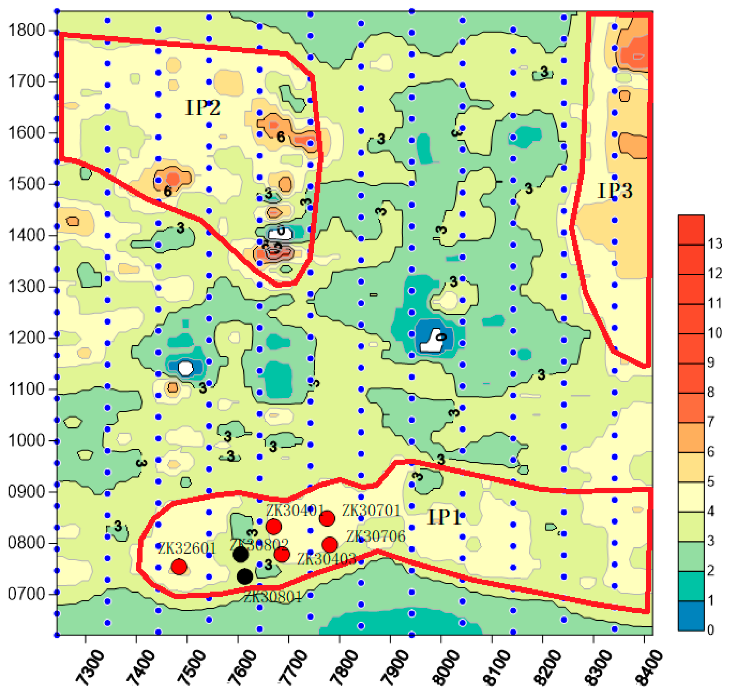
From the borehole data analysis, the anomaly IP1 has been separated into two parts. The lower IP area (<3) in the IP1 area has been drilled by two wells: ZK30802 and ZK30804. Unfortunately, we did not find any gold ore body or mineralization. In the Figure 6, Figure 7 and Figure 10, the SPDE, natural neighbor, and Kriging methods provided low IP anomalies. Compared to the natural neighbor and Kriging methods, the SPDE (Figure 6) showed more details. Because the owner only drilled in the IP1 area, the other two anomalies IP2 and IP3 have not been verified by the drilling wells. Figure 13 shows the borehole results of the drilled seven wells in IP1 area. The deepest well, ZK30701, has been drilled 347.4 m.

5. Conclusions and Future Work

The statistical model-based SPDE approach has been applied to predict the induced polarization field dataset. This approach constructs a statistical spatial model for geophysical dataset. Using this approach, the field data can be reconstructed and interpolated efficiently. The SPDE model can utilize the information from the dataset and return precise delineation of IP anomalies. The reason is that the statistical model considers the relationship among different data locations, and the modeled relationship fulfills the first law of geography which states “Everything is related to everything else, but near things are more related than distant things” [25]. The effectiveness and efficiency have been approved by the synthetic example. Then, we tested the method by a real field data case for the gold mineral exploration. The predicted values are quite close to the observed data. Compared to the natural neighbor interpolation, the nearest neighbor interpolation, the minimum curvature interpolation, and Kriging interpolation methods, the SPDE model-based method provided the smoothest and most accurate map. The borehole data have verified that the SPDE method gives more useful detailed information. The SPDE model-based method can provide the uncertainty of the prediction, and the uncertainty of the prediction is also obtained from the statistical model to help us in further research. In addition, we, in this paper, have fixed the value of parameter b. In practice, we can change this parameter to control the smoothness, as discussed in Lindgren et al. [12], and we retain this part for our future work.

Currently, we only considered a simple SPDE in constructing the model. One direction of our future work is to extend the statistical model to complex settings and to construct advanced statistical models. Deeper statistical analysis can also be used, but this might go far beyond the scope of this paper, and this is another direction of future work. In general, this approach might give us a new view of how to use the available dataset, and we are trying to use and integrate the proposed method to be applied in geology in the future.