Applying Electrical Resistivity Tomography in Ornamental Stone Mining: Challenges and Solutions

 , , ,
, , , 
Abstract
1. Introduction
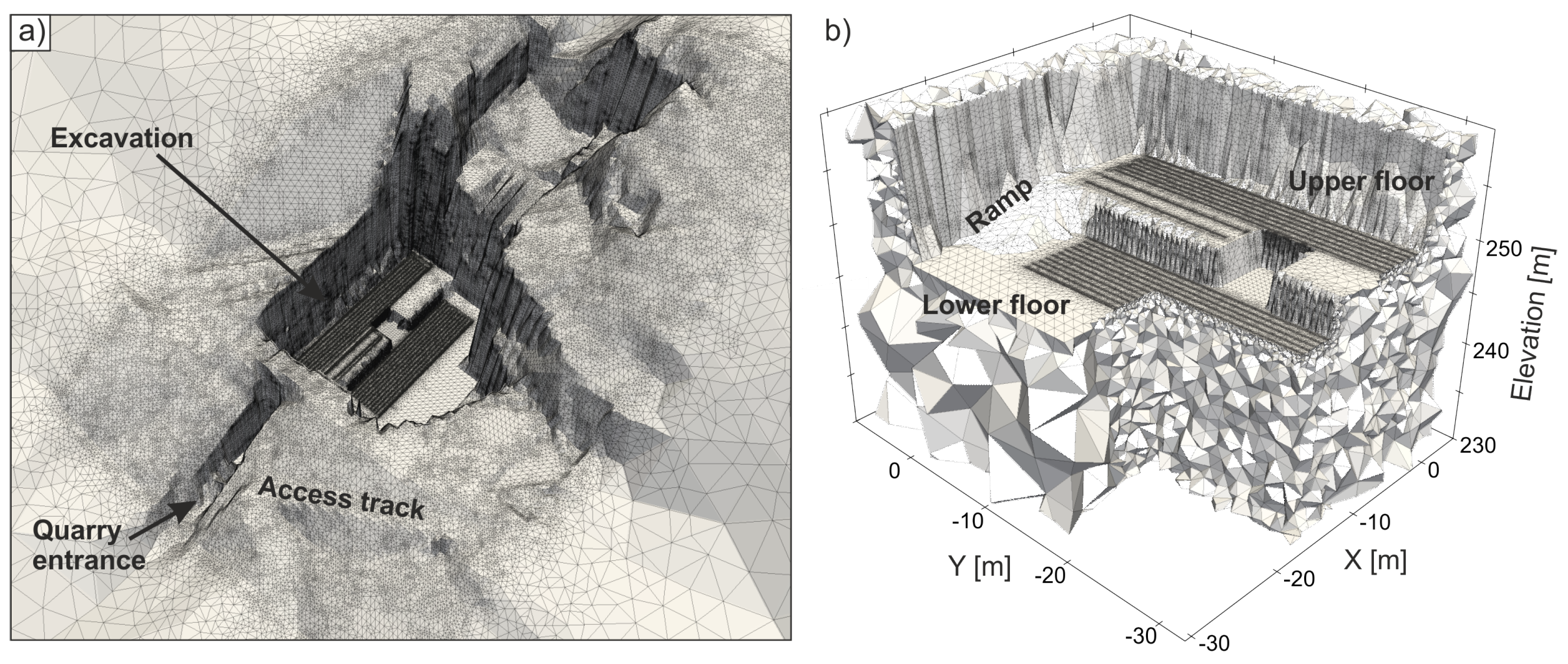
2. Study Site
3. Methodology
4. Challenges
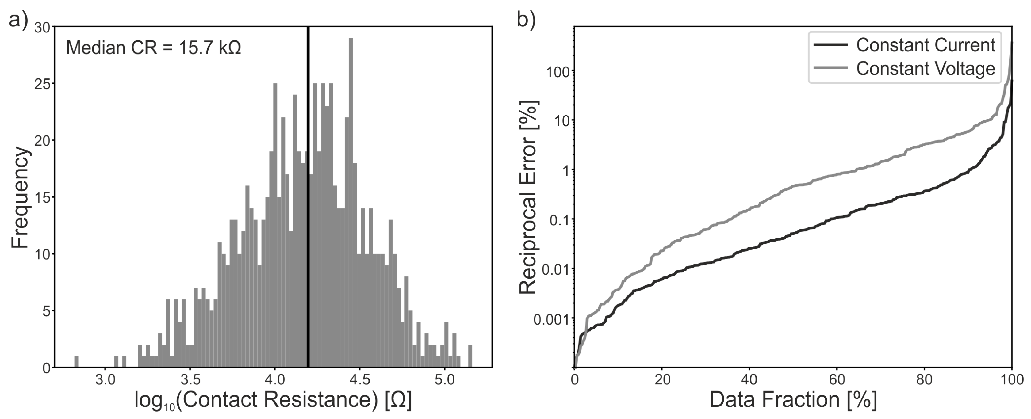
4.1. Contact Resistance
4.2. Topography
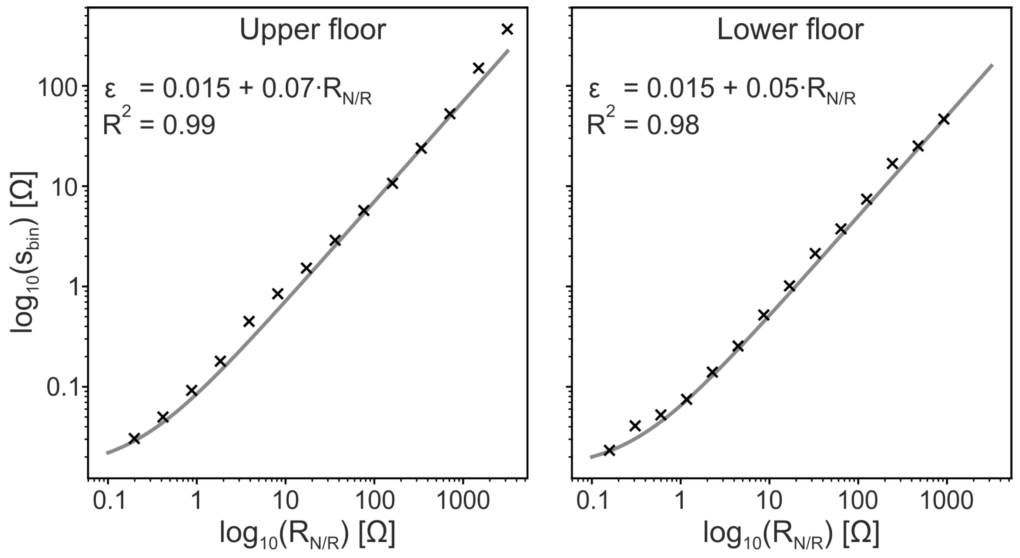
4.3. Data Inversion
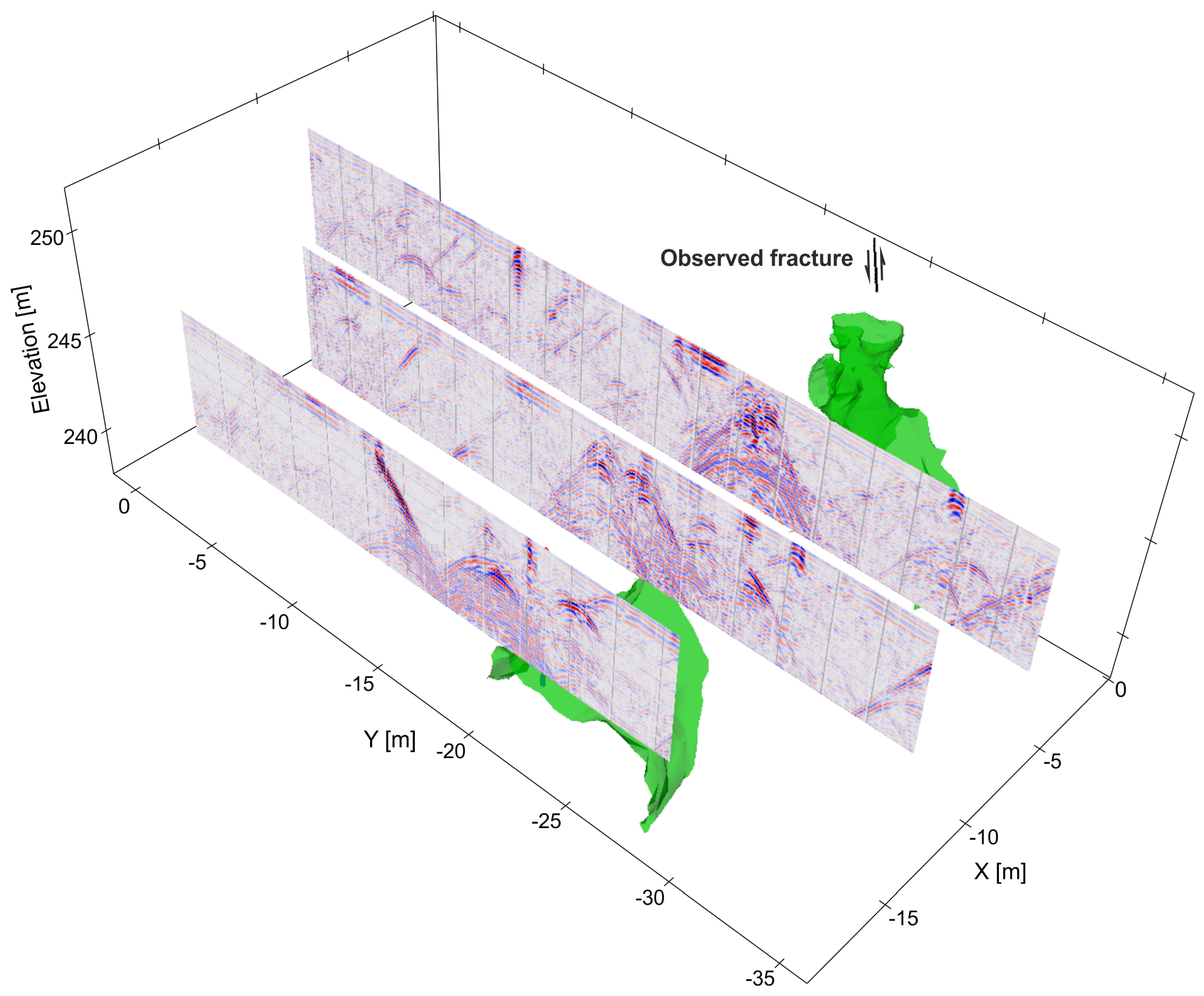
5. Results
6. Discussion
7. Summary and Conclusions
Author Contributions
Funding
Acknowledgments
Conflicts of Interest
References
- Dino, G.A.; Chiappino, C.; Rossetti, P.; Franchi, A.; Baccioli, G. Extractive Waste Management: A New Territorial and Industrial Approach in Carrara Quarry Basin. Ital. J. Eng. Geol. Environ. 2017, 2, 47–55. [Google Scholar] [CrossRef]
- Ashmole, I.; Motloung, M. Dimension Stone: The Latest Trends In Exploration And Production Technology. S. Afr. Inst. Min. Metall. 2008, 1, 35–70. [Google Scholar]
- Cosi, M. The dimension stone sector: New perspectives on the global market and on the reporting of international mining standards. Eur. Geol. 2015, 39, 24–30. [Google Scholar]
- EUROSTAT. Generation of Waste by Economic Activity; EUROSTAT: Luxembourg, 2018. [Google Scholar]
- Espín de Gea, A.; Reyes Urquiza, M.; Gil Abellán, A. Los métodos geofísicos como herramienta de mejora para el conocimiento y aprovechamiento de los yacimientos de roca ornamental. Boletín Geológico Y Minero 2017, 128, 363–378. [Google Scholar] [CrossRef]
- Telford, W.; Geldart, L.; Sheriff, R. Applied Geophysics, 2nd ed.; Cambridge University Press: Cambridge, UK, 1990. [Google Scholar]
- Luodes, H. Natural stone assessment with ground penetrating radar. Est. J. Earth Sci. 2008, 57, 149–155. [Google Scholar] [CrossRef]
- Luodes, H.; Sutinen, H.; Härmä, P.; Pirinen, H.; Selonen, O. Engineering Geology for Society and Territory—Volume 5: Urban Geology, Sustainable Planning and Landscape Exploitation; Springer International Publishing: Cham, Switzerland, 2015; Volume 5, pp. 243–246. [Google Scholar]
- Rey, J.; Martínez, J.; Vera, P.; Ruiz, N.; Cañadas, F.; Montiel, V. Ground-penetrating radar method used for the characterisation of ornamental stone quarries. Constr. Build. Mater. 2015, 77, 439–447. [Google Scholar] [CrossRef]
- Rey, J.; Martinez, J.; Montiel, V.; Canadas, F.; Ruiz, N. Characterization of the sedimentary fabrics in ornamental rocks by using GPR. Near Surf. Geophys. 2017, 15, 457–465. [Google Scholar] [CrossRef]
- Elkarmoty, M.; Colla, C.; Gabrielli, E.; Bonduà, S.; Bruno, R. A Combination of GPR Survey and Laboratory Rock Tests for Evaluating an Ornamental Stone Deposit in a Quarry Bench. Procedia Eng. 2017, 191, 999–1007. [Google Scholar] [CrossRef]
- Loke, M.H.; Chambers, J.E.; Rucker, D.F.; Kuras, O.; Wilkinson, P.B. Recent developments in the direct-current geoelectrical imaging method. J. Appl. Geophys. 2013, 95, 135–156. [Google Scholar] [CrossRef]
- Binley, A.; Hubbard, S.S.; Huisman, J.A.; Revil, A.; Robinson, D.A.; Singha, K.; Slater, L.D. The emergence of hydrogeophysics for improved understanding of subsurface processes over multiple scales. Water Resour. Res. 2015, 51, 3837–3866. [Google Scholar] [CrossRef] [PubMed]
- Magnusson, M.K.; Fernlund, J.M.; Dahlin, T. Geoelectrical imaging in the interpretation of geological conditions affecting quarry operations. Bull. Eng. Geol. Environ. 2010, 69, 465–486. [Google Scholar] [CrossRef]
- Chambers, J.E.; Wilkinson, P.B.; Wardrop, D.; Hameed, A.; Hill, I.; Jeffrey, C.; Loke, M.H.; Meldrum, P.I.; Kuras, O.; Cave, M.; et al. Bedrock detection beneath river terrace deposits using three-dimensional electrical resistivity tomography. Geomorphology 2012, 177–178, 17–25. [Google Scholar] [CrossRef]
- Chambers, J.E.; Wilkinson, P.B.; Penn, S.; Meldrum, P.I.; Kuras, O.; Loke, M.H.; Gunn, D.A. River terrace sand and gravel deposit reserve estimation using three-dimensional electrical resistivity tomography for bedrock surface detection. J. Appl. Geophys. 2013, 93, 25–32. [Google Scholar] [CrossRef]
- Hauck, C. Frozen ground monitoring using DC resistivity tomography. Geophys. Res. Lett. 2002, 29, 10–13. [Google Scholar] [CrossRef]
- Hauck, C.; Vonder Muhll, D.; Maurer, H. Using DC resistivity tomography to detect and characterize mountain permafrost. Geophys. Prospect. 2003, 51, 273–284. [Google Scholar] [CrossRef]
- Sass, O. Rock moisture fluctuations during freeze-thaw cycles: Preliminary results from electrical resistivity measurements. Polar Geogr. 2004, 28, 13–31. [Google Scholar] [CrossRef]
- Krautblatter, M.; Hauck, C. Electrical resistivity tomography monitoring of permafrost in solid rock walls. J. Geophys. Res. 2007, 112, 1–14. [Google Scholar] [CrossRef]
- Hilbich, C.; Hauck, C.; Hoelzle, M.; Scherler, M.; Schudel, L.; Völksch, I.; Vonder Mühll, D.; Mäusbacher, R. Monitoring mountain permafrost evolution using electrical resistivity tomography: A 7-year study of seasonal, annual, and long-term variations at Schilthorn, Swiss Alps. J. Geophys. Res. 2008, 113. [Google Scholar] [CrossRef]
- Hilbich, C.; Fuss, C.; Hauck, C. Automated Time-lapse ERT for Improved Process Analysis and Monitoring of Frozen Ground. Permafr. Periglac. Process. 2011, 22, 306–319. [Google Scholar] [CrossRef]
- Krautblatter, M.; Verleysdonk, S.; Flores-Orozco, A.; Kemna, A. Temperature-calibrated imaging of seasonal changes in permafrost rock walls by quantitative electrical resistivity tomography (Zugspitze, German/Austrian Alps). J. Geophys. Res. 2010, 115, 1–15. [Google Scholar] [CrossRef]
- Murton, J.B.; Kuras, O.; Krautblatter, M.; Cane, T.; Tschofen, D.; Uhlemann, S.; Schober, S.; Watson, P. Monitoring rock freezing and thawing by novel geoelectrical and acoustic techniques. J. Geophys. Res. Earth Surf. 2016, 121, 2309–2332. [Google Scholar] [CrossRef]
- Lesparre, N.; Boyle, A.; Grychtol, B.; Cabrera, J.; Marteau, J.; Adler, A. Electrical resistivity imaging in transmission between surface and underground tunnel for fault characterization. J. Appl. Geophys. 2016, 128, 163–178. [Google Scholar] [CrossRef]
- Caterina, D.; Orozco, A.F.; Nguyen, F. Long-term ERT monitoring of biogeochemical changes of an aged hydrocarbon contamination. J. Contam. Hydrol. 2017, 201, 19–29. [Google Scholar] [CrossRef] [PubMed]
- Robinson, J.; Johnson, T.; Slater, L. Challenges and opportunities for fractured rock imaging using 3D cross-borehole electrical resistivity. Geophysics 2015, 80, E49–E61. [Google Scholar] [CrossRef]
- ISPRA. Corna. In Carta Geologica d’italia 1:50.000—Catalogo delle Formazioni; ISPRA: Roma, Italy, 1992; pp. 71–105. [Google Scholar]
- Archie, G.E. The electrical resistivity log as an aid in determining some reservoir characteristics. Pet. Trans. AIME 1942, 146, 54–62. [Google Scholar] [CrossRef]
- Waxman, M.H.; Smits, L.J.M. Electrical conductivities in oil-bearing shaly sands. Soc. Pet. Eng. J. 1968, 8, 107–122. [Google Scholar] [CrossRef]
- Kaufmann, O.; Deceuster, J. Detection and mapping of ghost-rock features in the Tournaisis area through geophysical methods—An overview. Geol. Belg. 2014, 17, 17–26. [Google Scholar]
- Dubois, C.; Quinif, Y.; Baele, J.M.; Barriquand, L.; Bini, A.; Bruxelles, L.; Dandurand, G.; Havron, C.; Kaufmann, O.; Lans, B.; et al. The process of ghost-rock karstification and its role in the formation of cave systems. Earth-Sci. Rev. 2014, 131, 116–148. [Google Scholar] [CrossRef]
- Van Hoorde, M.; Hermans, T.; Dumont, G.; Nguyen, F. 3D electrical resistivity tomography of karstified formations using cross-line measurements. Eng. Geol. 2017, 220, 123–132. [Google Scholar] [CrossRef]
- Loke, M.H. Tutorial: 2-D and 3-D Electrical Imaging Surveys. Available online: https://sites.ualberta.ca/~unsworth/UA-classes/223/loke_course_notes.pdf (accessed on 26 July 2004).
- Chambers, J.E.; Ogilvy, R.; Kuras, O. 3D electrical imaging of known targets at a controlled environmental test site. Environ. Geol. 2002, 41, 690–704. [Google Scholar] [CrossRef]
- Loke, M.H.; Wilkinson, P.B.; Uhlemann, S.S.; Chambers, J.E.; Oxby, L.S. Computation of optimized arrays for 3-D electrical imaging surveys. Geophys. J. Int. 2014, 199, 1751–1764. [Google Scholar] [CrossRef]
- Gharibi, M.; Bentley, L.R. Resolution of 3-D Electrical Resistivity Images from Inversions of 2-D Orthogonal Lines. J. Environ. Eng. Geophys. 2005, 10, 339–349. [Google Scholar] [CrossRef]
- Athanasiou, E.; Tsourlos, P. Non-destructive DC resistivity surveying using flat-base electrodes. Near Surf. Geophys. 2007, 5, 263–272. [Google Scholar] [CrossRef]
- Rücker, C.; Günther, T. The simulation of finite ERT electrodes using the complete electrode model. Geophysics 2011, 76, F227–F238. [Google Scholar] [CrossRef]
- Martínez-Moreno, F.J.; Galindo-Zaldívar, J.; Pedrera, A.; Teixido, T.; Ruano, P.; Peña, J.A.; González-Castillo, L.; Ruiz-Constán, A.; López-Chicano, M.; Martín-Rosales, W. Integrated geophysical methods for studying the karst system of Gruta de las Maravillas (Aracena, Southwest Spain). J. Appl. Geophys. 2014, 107, 149–162. [Google Scholar] [CrossRef]
- Parsekian, A.D.; Claes, N.; Singha, K.; Minsley, B.J.; Carr, B.; Voytek, E.; Harmon, R.; Kass, A.; Carey, A.; Thayer, D.; et al. Comparing Measurement Response and Inverted Results of Electrical Resistivity Tomography Instruments. J. Environ. Eng. Geophys. 2017, 22, 249–266. [Google Scholar] [CrossRef]
- Supper, R.; Ottowitz, D.; Jochum, B.; Römer, A.; Pfeiler, S.; Gruber, S.; Keuschnig, M.; Ita, A. Geoelectrical monitoring of frozen ground and permafrost in alpine areas: field studies and considerations towards an improved measuring technology. Near Surf. Geophys. 2014, 12, 93–115. [Google Scholar] [CrossRef]
- Tsourlos, P.I.; Szymanski, J.E.; Tsokas, G.N. The effect of terrain topography on commonly used resistivity arrays. Geophysics 1999, 64, 1357–1363. [Google Scholar] [CrossRef]
- Wilkinson, P.B.; Chambers, J.E.; Meldrum, P.I.; Gunn, D.A.; Ogilvy, R.D.; Kuras, O. Predicting the movements of permanently installed electrodes on an active landslide using time-lapse geoelectrical resistivity data only. Geophys. J. Int. 2010, 183, 543–556. [Google Scholar] [CrossRef]
- Wilkinson, P.B.; Uhlemann, S.; Chambers, J.E.; Meldrum, P.I.; Loke, M.H. Development and testing of displacement inversion to track electrode movements on 3-D electrical resistivity tomography monitoring grids. Geophys. J. Int. 2014, 200, 1566–1581. [Google Scholar] [CrossRef]
- Wilkinson, P.B.; Chambers, J.; Uhlemann, S.; Meldrum, P.; Smith, A.; Dixon, N.; Loke, M.H. Reconstruction of landslide movements by inversion of 4-D electrical resistivity tomography monitoring data. Geophys. Res. Lett. 2016, 43, 1166–1174. [Google Scholar] [CrossRef]
- Uhlemann, S.; Wilkinson, P.B.; Chambers, J.E.; Maurer, H.; Merritt, A.J.; Gunn, D.A.; Meldrum, P.I. Interpolation of landslide movements to improve the accuracy of 4D geoelectrical monitoring. J. Appl. Geophys. 2015, 121, 93–105. [Google Scholar] [CrossRef]
- Boyle, A.; Wilkinson, P.B.; Chambers, J.E.; Meldrum, P.I.; Uhlemann, S.; Adler, A. Jointly reconstructing ground motion and resistivity for ERT-based slope stability monitoring. Geophys. J. Int. 2018, 212, 1167–1182. [Google Scholar] [CrossRef]
- Udphuay, S.; Günther, T.; Everett, M.E.; Warden, R.R.; Briaud, J.L. Three-dimensional resistivity tomography in extreme coastal terrain amidst dense cultural signals: application to cliff stability assessment at the historic D-Day site. Geophys. J. Int. 2011, 185, 201–220. [Google Scholar] [CrossRef]
- Cho, I.; Ha, I.; Kim, K.; Ahn, H. 3D Effects on 2D Resistivity Monitoring in Earth-fill Dams. Near Surf. Geophys. 2013, 11, 1–10. [Google Scholar] [CrossRef]
- Si, H. TetGen: A Quality Tetrahedral Mesh Generator and Three-Dimensional Delaunay Triangulator; WIAS: Berlin, Germany, 2006. [Google Scholar]
- Johnson, T.C.; Versteeg, R.J.; Ward, A.; Day-Lewis, F.D.; Revil, A. Improved hydrogeophysical characterization and monitoring through parallel modeling and inversion of time-domain resistivity and induced-polarization data. Geophysics 2010, 75, WA27–WA41. [Google Scholar] [CrossRef]
- Koestel, J.; Kemna, A.; Javaux, M.; Binley, A.; Vereecken, H. Quantitative imaging of solute transport in an unsaturated and undisturbed soil monolith with 3-D ERT and TDR. Water Resour. Res. 2008, 44. [Google Scholar] [CrossRef]
- Takahashi, K.; Igel, J.; Preetz, H.; Kuro, S. Basics and Application of Ground-Penetrating Radar as a Tool for Monitoring Irrigation Process. In Problems, Perspectives and Challenges of Agricultural Water Management; InTech: Vienna, Austria, 2012. [Google Scholar]
- Maurer, H.; Friedel, S. Outer-space sensitivities in geoelectrical tomography. Geophysics 2006, 71, G93–G96. [Google Scholar] [CrossRef]
- Loke, M.H.; Wilkinson, P.B.; Chambers, J.E. Parallel computation of optimized arrays for 2-D electrical imaging surveys. Geophys. J. Int. 2010, 183, 1302–1315. [Google Scholar] [CrossRef]


© 2018 by the authors. Licensee MDPI, Basel, Switzerland. This article is an open access article distributed under the terms and conditions of the Creative Commons Attribution (CC BY) license (http://creativecommons.org/licenses/by/4.0/).
Share and Cite
Uhlemann, S.; Chambers, J.; Falck, W.E.; Tirado Alonso, A.; Fernández González, J.L.; Espín de Gea, A. Applying Electrical Resistivity Tomography in Ornamental Stone Mining: Challenges and Solutions. Minerals 2018, 8, 491. https://doi.org/10.3390/min8110491
Uhlemann S, Chambers J, Falck WE, Tirado Alonso A, Fernández González JL, Espín de Gea A. Applying Electrical Resistivity Tomography in Ornamental Stone Mining: Challenges and Solutions. Minerals. 2018; 8(11):491. https://doi.org/10.3390/min8110491
Chicago/Turabian StyleUhlemann, Sebastian, Jonathan Chambers, W. Eberhard Falck, Avelino Tirado Alonso, José Luis Fernández González, and Antonio Espín de Gea. 2018. "Applying Electrical Resistivity Tomography in Ornamental Stone Mining: Challenges and Solutions" Minerals 8, no. 11: 491. https://doi.org/10.3390/min8110491
APA StyleUhlemann, S., Chambers, J., Falck, W. E., Tirado Alonso, A., Fernández González, J. L., & Espín de Gea, A. (2018). Applying Electrical Resistivity Tomography in Ornamental Stone Mining: Challenges and Solutions. Minerals, 8(11), 491. https://doi.org/10.3390/min8110491