Kriging Interpolation for Evaluating the Mineral Resources of Cobalt-Rich Crusts on Magellan Seamounts

Abstract

The evaluation of mineral resources on seamounts by geostatistics faces two key challenges. First, the conventional distance/orientation- and the simple distance-based variogram functions used are ineffective at expressing the spatial self-correlation and continuity of cobalt-rich crust thicknesses on seamounts. Second, the sampling stations used for a single seamount are generally very sparsely distributed because of the high survey costs, which results in an insufficient number of information points for variogram fitting. Here, we present an alternative geostatistical method that uses distance/gradient- and distance/relative-depth-based variograms to process data collected from several neighboring seamounts, allowing the variogram fitting. The application example reported for the Magellan seamounts demonstrates the suitability of the method for evaluating the mineral resources of cobalt-rich crusts. The method could be effective also for the analysis of surface data obtained from mountain slopes on land (e.g., soil).

1. Introduction

Seamounts are submarine volcanogenic conical or flat-topped mountains (the latter are called guyots) rising hundreds or thousands of meters from the seafloor, sometimes emerging above the sea level to form islands, and covering large areas (up to 10,000 km² each). Cobalt-rich crusts form on the sediment-free surfaces of seamount slopes and summits, being of significant economic interest because of the potential presence of manganese, cobalt, nickel, tellurium, platinum, and other rare earth elements [1,2,3]. Therefore, several explorative and resource evaluation campaigns are currently conducted on seamounts.

Since the distribution of sampling stations on seamounts tends to be sparse owing to the costs of the survey cruises, the spatial interpolation of the collected data represents a critical issue for both scientific research and industrial exploration. Window averaging, distance inverse weighting, simple average values, and geostatistics have been generally used for spatial interpolation. Among the interpolation methods, kriging is nowadays a typical choice for quantifying mineral reserves because it provides the best linear unbiased predictions [4,5,6].

Distribution of cobalt-rich crusts on seamount surfaces are influenced by the water depth [1,7,8] but, to the best of our knowledge, no study has proven that they are influenced by the direction. Kriging with conventional variograms [6,9,10,11,12,13,14,15,16], including orientation-based ones, has proven ineffective at quantifying mineral resources on seamounts [17]. This is probably why kriging is not among the methods commonly used for seamount interpolation mentioned above [18].

A new method using distance/gradient-based variograms has been recently proposed by Du et al. [17] and is preliminarily used for the evaluation of seamount mineral resources [19]. Despite its demonstrated efficiency in spatial interpolation for seamounts [17], some significant problems arise when using it. First, kriging interpolation must face the expensiveness of survey cruises for deep sea exploration and the consequent sparse distribution of the sampling stations, which results in an insufficient number of information points for variogram fitting, the solution for this problem was not presented in Du et al., 2017 [17]. Second, the fitting of distance/gradient-based variograms is more complicated than that of conventional ones and is difficult to use widely.

In this study, we aim to promote the use of kriging interpolation for seamounts. First, the method for unifying data collected from multiple seamounts to fit variograms for kriging interpolation on one guyot is described. Next, the distance/gradient-based variogram is reintroduced, and an alternative one (i.e., the distance/relative-depth-based variogram), which is easier for experimentation and variogram fitting and is similarly effective, is presented for the first time. Then, the processing of surveying data for several guyots from the Magellan seamounts with the above methods is discussed. Last, the kriging interpolation is compared with several non-geostatistical interpolation methods in order to demonstrate its effectiveness for the application to seamounts.

2. Data

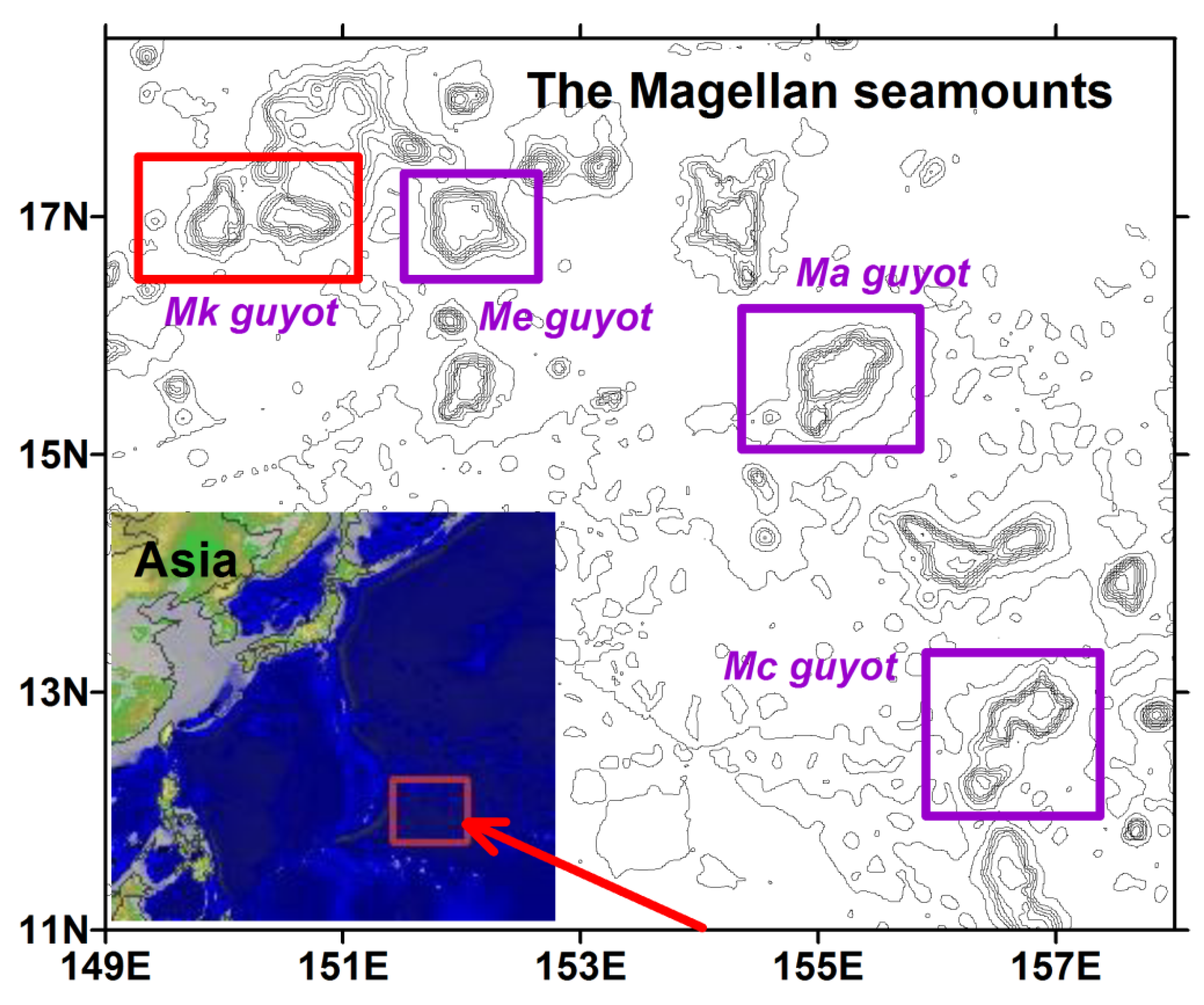
Since the 1990s, the Magellan seamounts, which are located in the Western Pacific Ocean (Figure 1), have been investigated by geologists from the China Ocean Mineral Resources Association (COMRA) as promising cobalt-rich crust deposits. Hence, we selected four guyots (Me, Mk, Ma, and Mc) from the Magellan seamounts to serve as application examples of the geostatistical methods that have been described above.

The bathymetric data for these guyots were obtained using a Simrad EM120 multibeam echo sonar (Kongsberg Underwater Technology Inc., Lynnwood, WA, USA) with a grid size of 100 × 100 m. The data for the cobalt-rich crust thicknesses were obtained by geological sampling, primarily via submarine drilling and dredging. The total number of sampling stations used for these four guyots was 264, and the water depth from sea level ranged from 1350 m to 3600 m. The spatial distributions of the cobalt-rich crusts were observed to be similar among the four seamounts [18].

Guyot Mk was used as the primary seamount that was to be interpolated via kriging, whereas the remaining three were subsequently added to the experiment to assess the accuracy with which they fitted the resulting variogram.

Table 1. Original and unified parameters of the cobalt-rich crust thickness of the four selected guyots.

Statistic Parameters	Guyots
	Mk	Me	Ma	Mc	Unified Data
Original mean (mm)	58	66	74	122
Transformed mean (mm)	58	58	58	58	58
Original standard deviation (mm)	33	35	38	73
Transformed standard deviation (mm)	33	31	30	35	32
Transformed weighting (Ti)	1.00	0.88	0.79	0.48
Number of samples	77	73	69	45	264

presents the statistical parameters of the cobalt-rich crusts. The significant difference between the average crust thicknesses of the four guyots indicates that it is unreasonable to simply combine (i.e., average) their data.

3. Materials and Methods

In this section, we present two key aspects of the proposed geostatistical method. First, we describe two adapted distance/depth-based variograms: distance/gradient- and distance/relative-depth-based variograms. Then, we unify data collected from multiple seamounts to obtain a variogram to use for the kriging interpolation of cobalt-rich crusts on a seamount.

3.1. Distance/Depth-Based Variograms

A perfectly conical seamount could be represented by a Lambert conformal coordinate system, but a local coordinate system can always be defined for any more complex surface, such as the guyots of the Magellan seamounts. Based on such a local coordinate system, one can build a conformal grid where the variogram is calculated and the kriging interpolation is performed. This operation consists in computing the variogram in a Riemannian space instead of a Euclidean one. This method has been investigated since 1998 [20] and is still used in the oil and gas field for estimating the variogram along non-flat faulted layers [21,22]. In a similar way, kriging methods for evaluating cobalt-rich crusts on seamounts are presented as follows.

3.1.1. Distance/Gradient-Based Variogram

By defining a local coordinate system u = {u(x, y, dp)} on the surface of seamounts, where (x, y) and dp are, respectively, the geographical coordinates and the depth of a spatial variable, such as the thickness of cobalt-rich crusts notated as Z(u), the variogram equation can be written as γ(h) = ½E([Z(u + h) − Z(u)]²), where h denotes the distance of geographical coordinates or differences of depth between two points in the coordinate system u.

Since $Z(u)=Z(x_i,y_i,d{p}_i),i=1,\dots ,n$ represents the thickness data for cobalt-rich crusts on a seamount surface at a geographic position $(x_t,y_i)$ with a water depth $d{p}_t$, the distance/gradient-based variogram is defined as half the arithmetic mean of the variance of data pairs given by the distance/gradient [17], which can be expressed as:

$$\gamma (h)=\gamma (dis,g)=\frac{1}{2N(dis,g)}\times {{\displaystyle \sum _{i=1,\dots ,n,j=1\dots ,n}^{N(dis,g)}[Z(x_i,y_i,d{p}_i)-Z(x_j,y_j,d{p}_j)]}}^2$$

(1)

where $dis=sqrt[{(x_i-x_j)}^2+{(y_i-y_j)}^2]$, $g=\arctan (\left|d{p}_i-d{p}_j\right|/dis)$ is the gradient of the seamount slope, and $N(dis,g)$ is the number of point pairs in the group $(dis,g)$.

3.1.2. Distance/Relative-Depth-Based Variogram

Here, we define the distance/relative-depth-based variogram as half the arithmetic mean of the variance of data pairs given by the distance and relative depth, which can be expressed as:

$$\gamma (dis,\Delta dp)=\frac{1}{2N(dis,\Delta dp)}\times {{\displaystyle \sum _{i=1,\dots ,n,j=1\dots ,n}^{N(dis,\Delta dp)}[Z(x_i,y_i,d{p}_i)-Z(x_j,y_j,d{p}_j)]}}^2$$

(2)

where $\Delta dp=\left|d{p}_i-d{p}_j\right|$.

3.2. Unifying Data from Multiple Seamounts

As noted above, the sparse distribution of sampling stations owing to the high survey costs results in an insufficient number of information points. Since such so-obtained calculation results are not ideal, for our application test, we selected several seamounts adjacent to each other with similar distribution characteristics in terms of cobalt-rich crust thickness, that is, the guyots Mk, Me, Ma, and Mc on the Magellan seamounts (Figure 1). Then, we unified the data collected from each of these seamounts, for experiments and variogram fitting using the kriging interpolation method, as follows:

First, we divided the average value of the data sampled from one seamount (e.g., guyot Mk) to be interpolated by kriging by the average value of those collected from another one (i.e., guyot Me, Ma, or Mc). The resulting quotient, expressed as $T_i=mea{n}_{Mk}/mea{n}_i,i=Mk,Me,Ma,Mc$, served as a weighting coefficient to transform the unified data.

By supposing that the unified data are $Z_{i,j}(i=Mk,Me,Ma,Mc;j=1,2,\dots ,N_i)$, where $N_i$ is the number of data points for a seamount i, those from the selected seamounts can be described as:

$$Z_{i,j}^{\ast }=T_i\times Z_{i,j}(i=Mk,Me,Ma,Mc;j=1,\dots ,N_i)$$

(3)

4. Results

4.1. Unified Data from Four Guyots on the Magellan Seamounts

The datasets (i.e., cobalt-rich crusts thickness) from different seamounts exhibit different mean and standard deviation values (shown in Table 1) probably because of their different geological ages and environments; furthermore, it seems that we cannot directly use all the data together because of the non-stationarity of the data between different mounts. We attempt to transform the datasets from different mounts and form new datasets that exhibit similar mean and standard deviation values; furthermore, we combine these datasets to obtain stationary unified datasets.

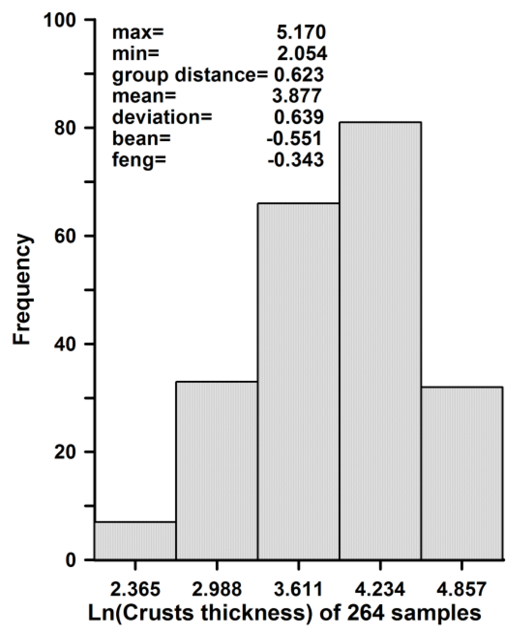
Using Equation (3), we obtained 264 unified data points from the statistical parameters shown in Table 1, and they had the same average values and approximate average deviations. Statistical tests revealed that the unified data followed a natural logarithm normal distribution, as shown in Figure 2. Thus, after logarithmic transformation, they were considered as weakly stationary random variables for variogram experiments [5]. Hence, this set of 264 data points, once transformed into natural logarithm values, can be used for experiments and variogram fitting of cobalt-rich crust thicknesses on the Magellan seamounts.

4.2. Experimental Variogram

4.2.1. Distance/Gradient-Based Variogram

For the distance search, we followed the approach described by Deutsch and Journel [23], while we divided the gradients into three groups on the basis of the one reported by Du et al. [17]. Pairs of sampling stations within a specific lag distance were selected according to both the lag distance and the tolerance. Then, the eventual statistical lag distance was taken as the mean of each group. Due to the same frequencies of point pairs occurring within certain gradient intervals, all point pairs were divided into three groups. Hence, for dis and g, we obtained N pairs and the variogram was calculated using Equation (1). Here, dis and g indicate the mean distance and gradient, respectively, of each group. As a result, the variogram for the three gradient groups was derived.

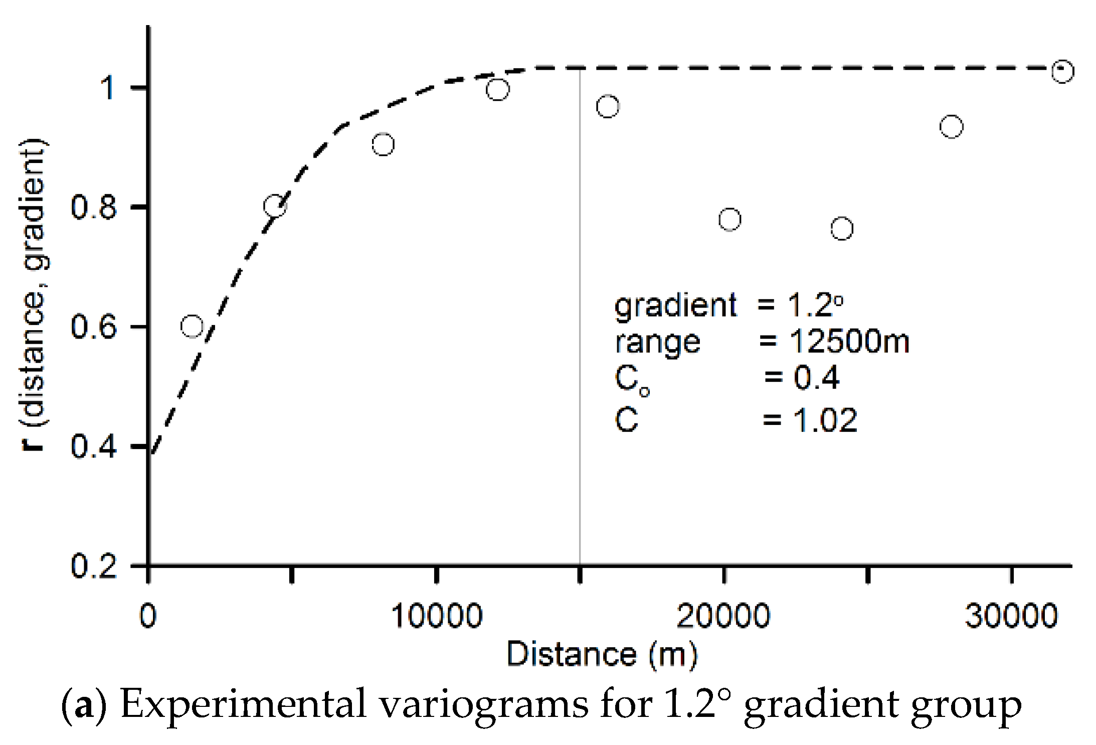
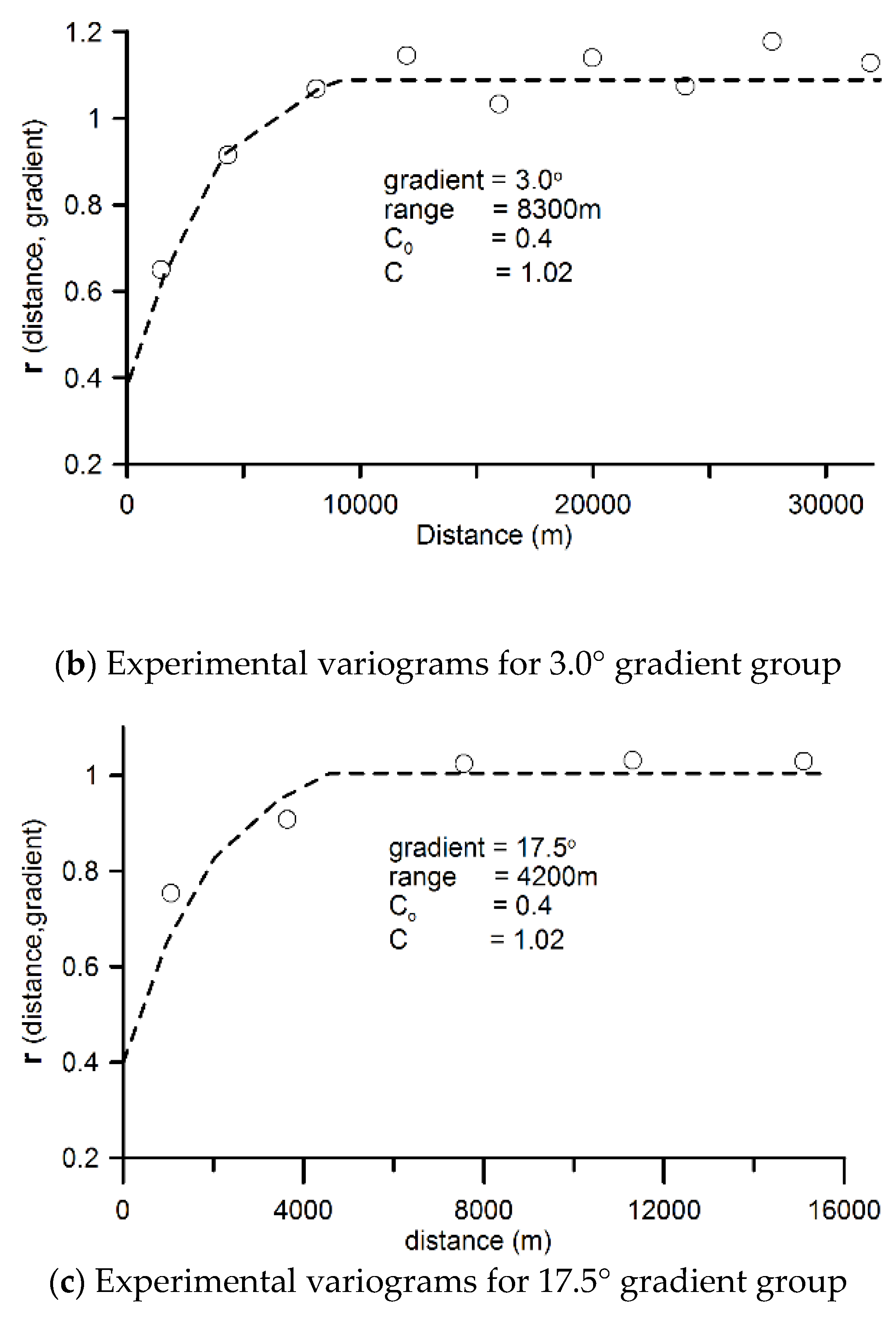
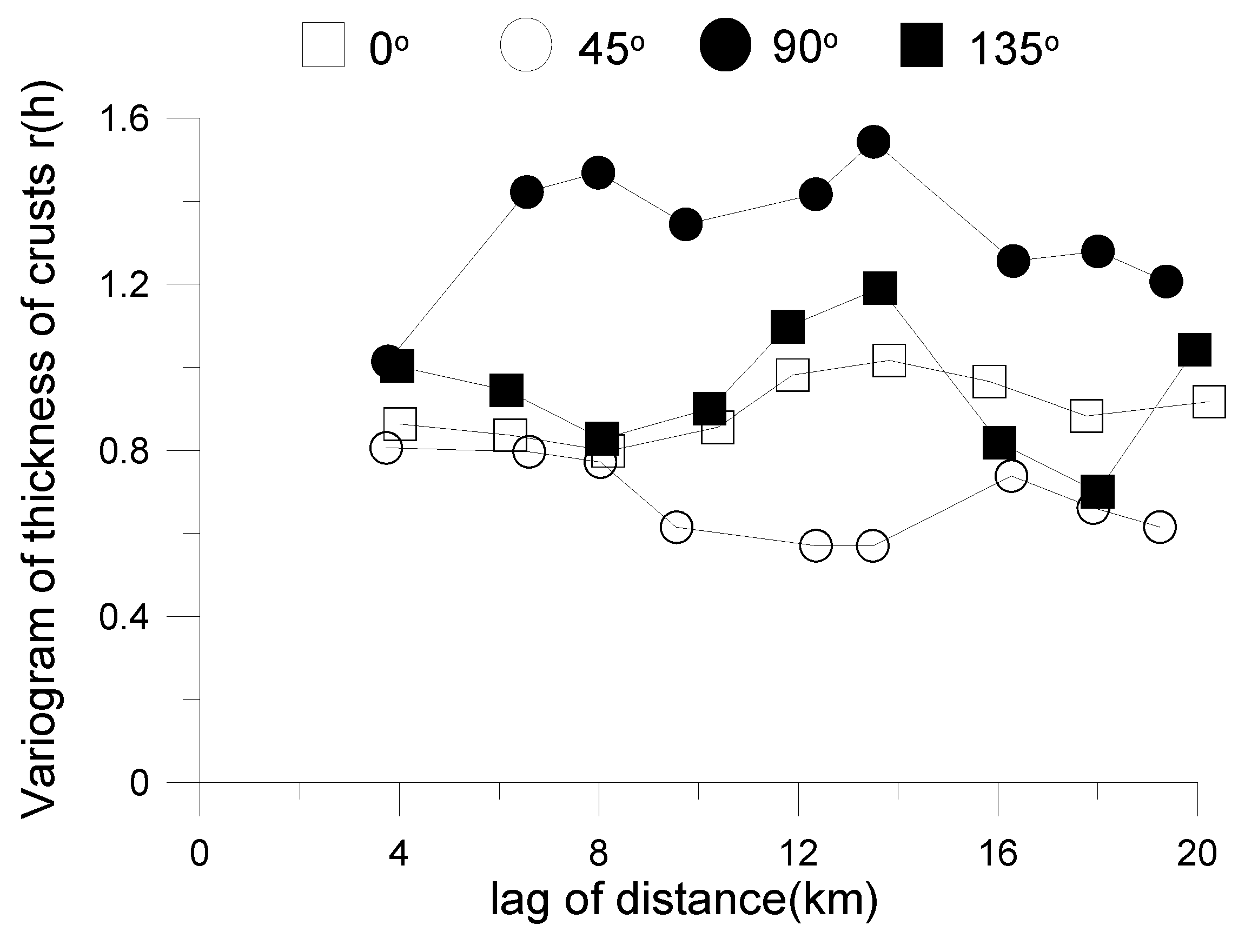
Figure 3 shows the distance/gradient-based variogram of cobalt-rich crust thicknesses for the unified data, demonstrating its effectiveness at describing the self-correlation of mineral resources on seamounts, whereas the distance/orientation-based variogram shown in Figure 4 seems ineffective.

Despite the different mean gradients and ranges between the three, the mean square deviations and the nugget effect were about 1.02 and 0.4, respectively, for all of them (Figure 3). Compared with the experimental distance/direction-based variogram [17], the distance/gradient-based algorithm clearly better applies to mineral resource data on seamount slopes.

4.2.2. Distance/Relative-Depth-Based Variogram

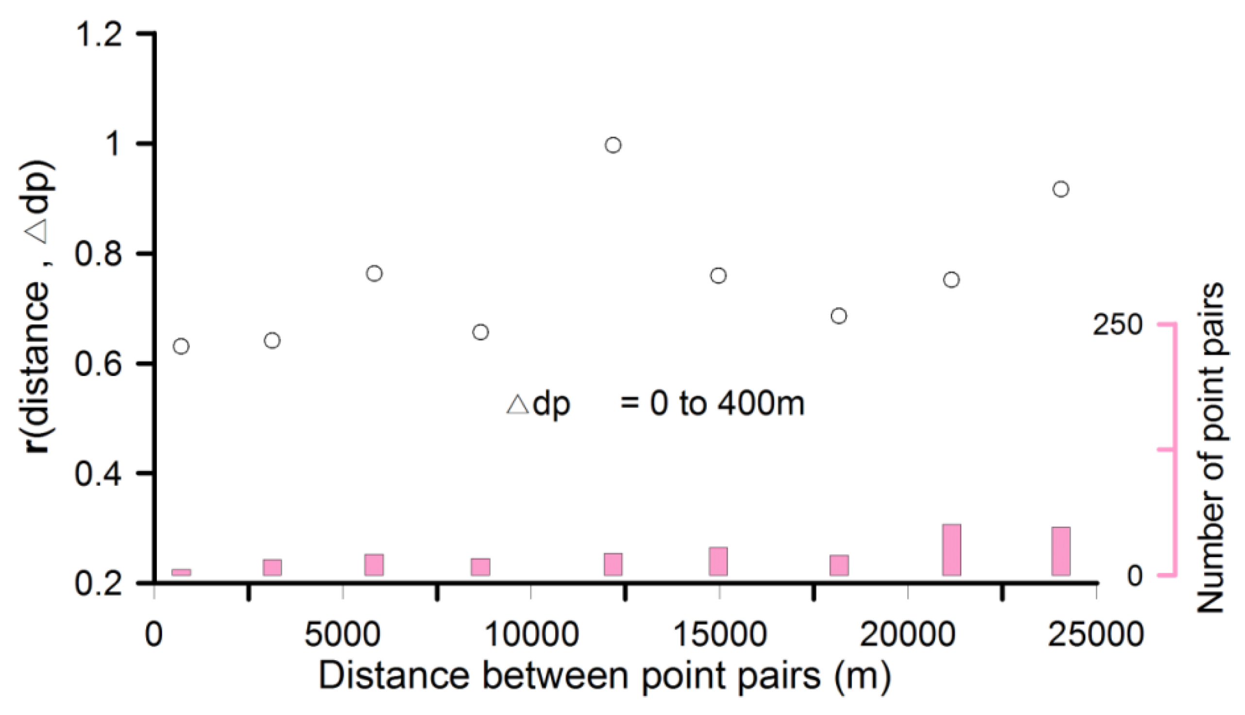
Our experiment on the distance/relative-depth-based variogram was similar to that on the distance/gradient-based one. The key difference was the placement of the gradient groups at relative-depth intervals, such as 100 m, 200 m, 300 m, 400 m, and 500 m, as calculated in Equation (2). Distance-based variogram fittings were performed in each relative-depth interval for the conventional variogram model. Intervals larger than 400 m exhibited no spatial correlation, and lower ones had insufficient data pairs, whereas the 400 m intervals (0–400 m, 400–800 m, and 800–1200 m) were suitable for the variogram calculation in this study.

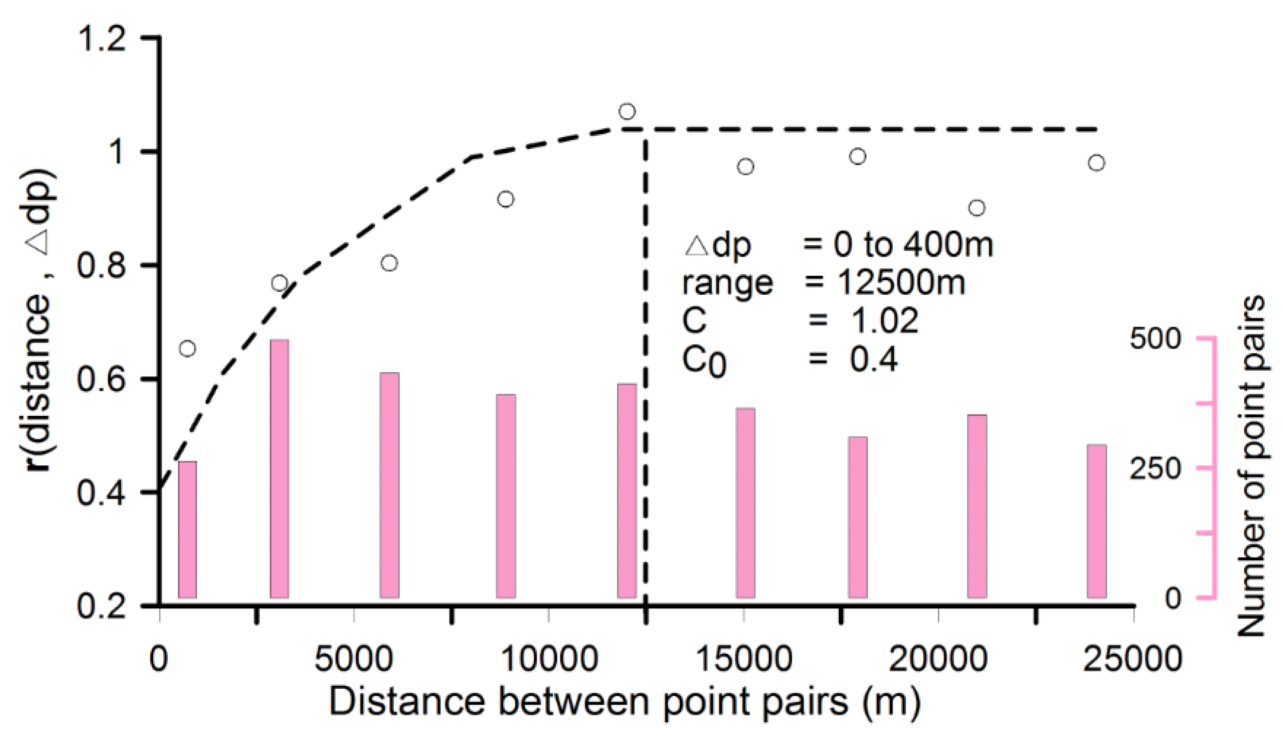
Figure 5 shows the experimental distance-based variogram for the 0–400 m relative-depth interval, whereas the other variograms with the 400 m interval (e.g., 400–800 m and 800–1200 m) were all ineffective. Hence, in such situations, only the variogram with a relative-depth interval ranging from 0 m to 400 m can be used for kriging interpolation.

The fitting and kriging processes for the distance/relative-depth-based variogram were the same as for conventional variograms. The following section shows how the two distance/depth-based variograms were fitted.

Furthermore, we have to say that distance/relative-depth-based variogram when one relative-depth interval was involved was observed to be equivalent to the conventional variogram in which the searching of point pairs was restricted in a relative-depth interval.

4.3. Variogram Fitting

4.3.1. Distance/Relative-Depth-Based Variogram Fitting

The distance/relative-depth-based variogram could be fitted with the same method used for traditional spherical model functions [23] as follows:

$$\gamma (h)=C_o+(C-C_o)Sph(h/a)=\{\begin{array}{c}{C}_o+(C-C_o)\left[1.5h/a-0.5{(h/a)}^3\right],ifh\le a\\ Cifh\ge a\end{array}$$

(4)

Here, h is equivalent to $(dis,\Delta depth)$, a is equivalent to range. Thus, the aforementioned equation can be transformed as follows:

$$\gamma (dis,\Delta depth)=C_o+(C-C_o)\times (1.5\times dis/range-0.5\times {(dis/range)}^3)$$

(5)

when $dis\le range$ and $\gamma (dis,\Delta depth)=c$ when $dis>range$. where C = 1.02, C₀ = 0.4, range = 12,500 m, and Δdepth = 0–400 m are deduced from the variograms shown in Figure 4.

4.3.2. Distance/Gradient-Based Variogram Fitting

● Gradient/Range Function

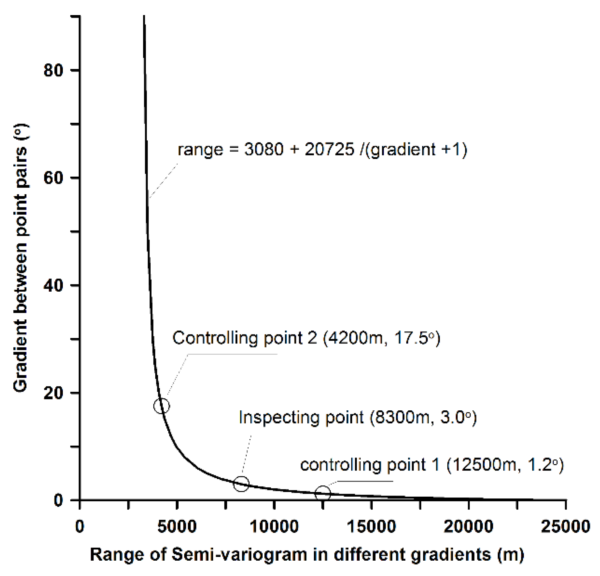
Only when gradient ranges are fitted to a continuous function can we consider the fitting of our theoretical variogram and apply kriging interpolation. Both Gendzwill and Stauffer and Deutsch and Journel [23,24] attempted to fit the anisotropy of ranges with spheroidal functions using polar coordinates. However, we used the Cartesian coordinate system and three groups of gradients/ranges: (1.2°, 12,500 m), (3.0°, 8300 m), and (17.5°, 4200 m). We obtained these results using the experimental variogram function described by Equation (1) and shown in Figure 4, where the range is virtually inversely proportional to the gradient. Furthermore, two of the groups were used as control points for fitting to the following equation:

$$range=a_o+p/(g+1)$$

(6)

where $a_0$ and p are constants, whereas the third group serves as an inspection point after the fitting.

Finally, we deduced the gradient/range fitting function as follows:

$$range=3080+20725/(g+1)$$

(7)

and the corresponding diagram is shown in Figure 6.

● Variogram Function Fitting

The gradient/range function expressed by Equation (6), obtained by fitting, was substituted into the theoretical variogram model represented by Equations (7) and (8), which was proposed by Deutsch and Journel [23] as a spherical, an exponential, or a Gaussian model. For our demonstration, we used the spherical model function.

$$\gamma (dis,g)=C_o+(C-C_0)\times Sph(dis/range)$$

(8)

that is:

$$\gamma (dis,g)=C_o+(C-C_o)\times (1.5\times dis/range-0.5\times {(dis/range)}^3)$$

(9)

when $dis\le range$ and $\gamma (dis,g)=c$ when $dis>range$. where C is the sill value or variance contribution, which in this example is 1.02, and C₀ is the nugget effect, set to 0.4. These values were deduced from the variograms shown in Figure 3.

The prominent feature of the above-mentioned theoretical variogram is that it is subject to a gradient rather than to an orientation; therefore, it is a function of distance and gradient.

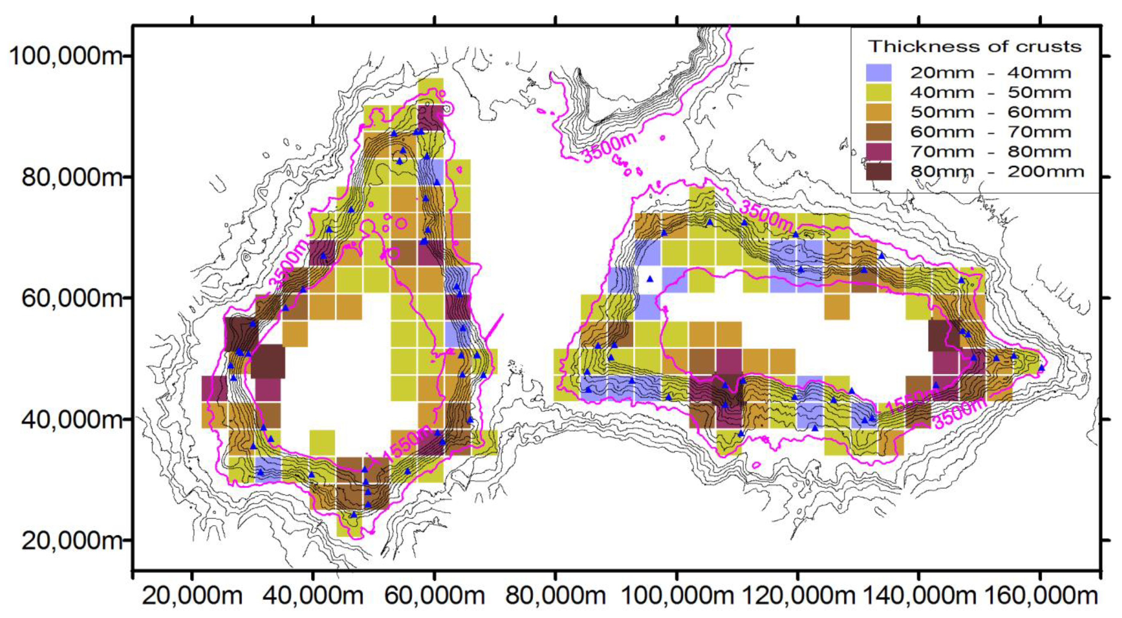
4.4. Estimating the Cobalt-Rich Crust Thicknesses on Guyot Mk

With the distance/relative-depth-based variogram, we used ordinary kriging interpolation method on a 3 × 3 block with 4472 × 4472 m unit squares and a horizontal area of 20 km², which is equivalent to the minimum grid unit area required by the Regulations on Prospecting and Exploration for Cobalt-Rich Crusts issued by the International Seabed Authority (ISA) [18]. Each location had a search radius of 12,000 m. Information points from neighboring locations were used in the interpolation (a maximum of nine and a minimum of three).

Natural logarithm values of 77 sampling data points for guyot Mk were taken as information points. The natural logarithm values of cobalt-rich crust thicknesses for 169 grid cells were estimated via kriging interpolation and using our geostatistical scheme. Antilog values of the estimated values are shown in Figure 7 as the distribution of the cobalt-rich crust thicknesses.

5. Discussion

5.1. Experimental Variogram on Unification Seamounts Compared with that on a Single Seamount

The same parameters of searching point pairs, i.e., lag separation distance of 3000 m, lag tolerance of 1500 m, relative depth interval of 0–400 m, are used in following two cases. When datasets from single seamount (e.g., Mk guyot, shown in Table 1) is used to calculate the experimental variogram, the number of point pairs in nine lags are 6–74, and the distribution of scatter dots exhibits the ineffectiveness of the experimental variogram (shown in Figure 8). However, datasets from unification seamounts (shown in Table 1) show that the number of point pairs in nine lags are 202–497, and the dotted curve exhibits the effectiveness of the experimental variogram (shown in Figure 5).

The ineffectiveness of the experimental variogram (shown in Figure 8) was probably arising because of the insufficient number of surveying data on single seamount. Unifying datasets from unification seamounts brought sufficient number of data, thereby figuring out the effectiveness of the experimental variogram (shown in Figure 5).

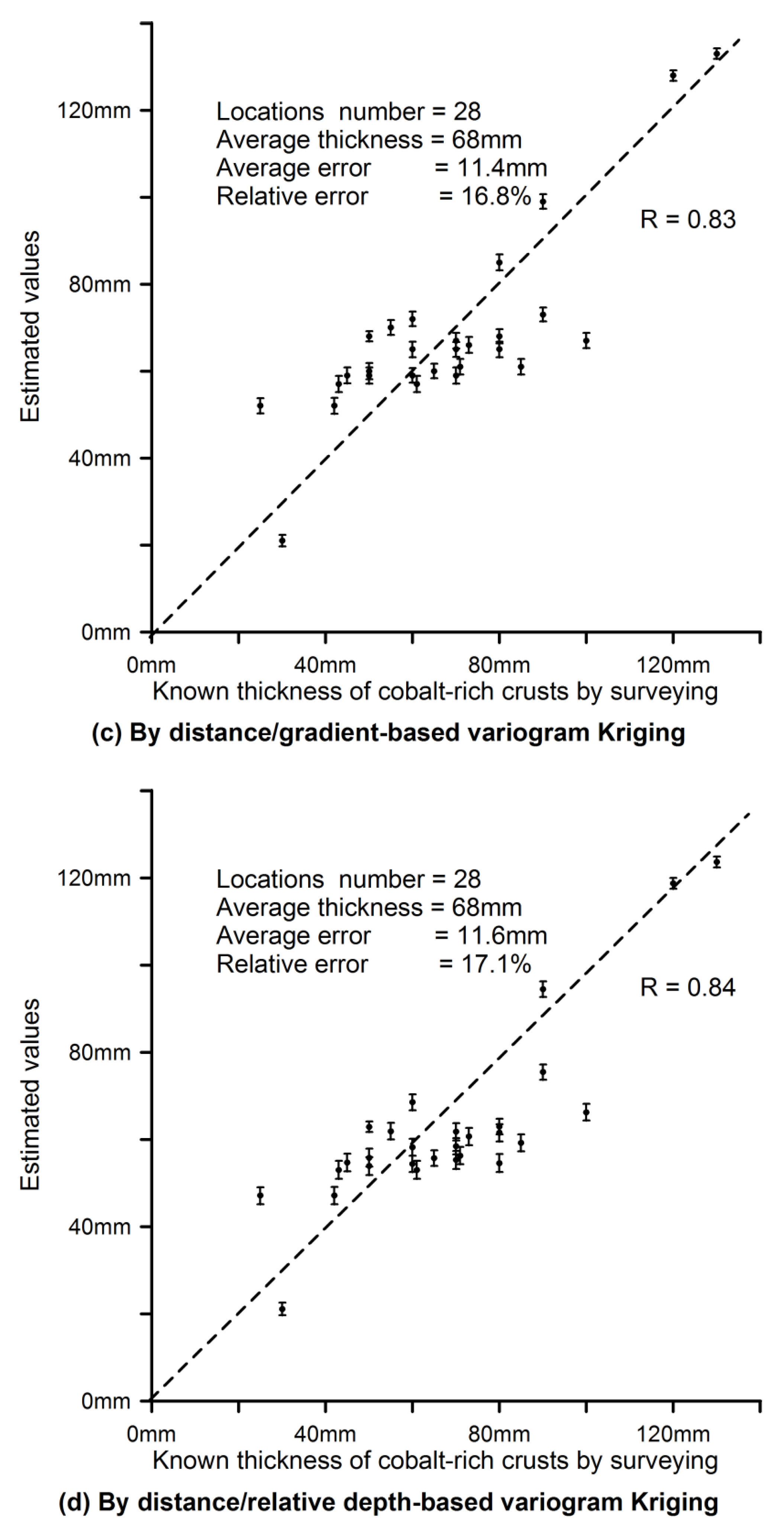
5.2. Kriging Compared with Other Interpolation Methods on Surveying Locations

We compared the method with several interpolation methods. Due to the sparse distribution of the sampling stations, assigning average values for all survey data (i.e., for guyot Mk, 58 mm in Table 1) to all grid nodes is a common method for evaluating the mineral resources on seamounts [18]. All the data were supposed to be predicted by this average value. As a result, the estimated average error was equal to the standard deviation of all data (i.e., for guyot Mk, 33 mm in Table 1), and the relative error was 56.9% (i.e., 33 mm/58 mm × 100%). These values served as reference points for evaluating the interpolation effects with other more complex methods.

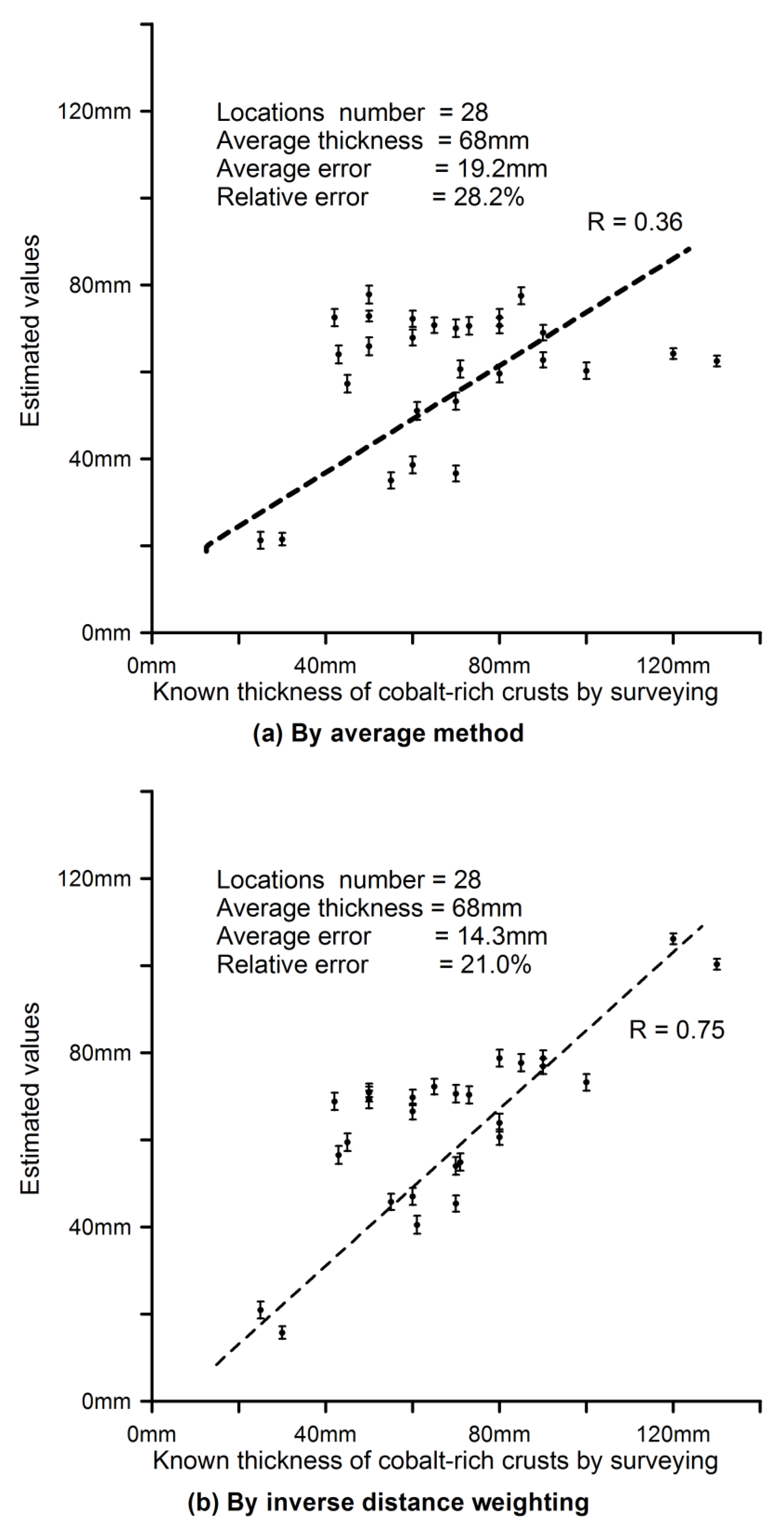
In order to compare these interpolation effects with those of our kriging interpolation, we also considered the window averaging, the inverse distance weighting, and distance/gradient-based variogram kriging methods. We used the same interpolation parameters (i.e., the same search radius (here, it is 12 km) and information point number) with each method. Each location with known surveying data was estimated with each of them.

Invalid interpolation stations were sometimes not encircled by information points so that they could not form a proper interpolation. Furthermore, in some cases, the locations and their neighboring information points were at different slopes, and they were considered as either impacted by a landslide or covered by sediments. Herein, the natural mechanical processes of seamount slope development destroyed the continuity of the cobalt-rich crusts, which resulted to be unpredictable via interpolation in some locations. Unlike the invalid interpolation stations, each effective interpolation station was encircled by information points and formed a sound interpolation. Furthermore, the information points were all located on relatively stable slopes without obvious landslide or sediment cover history.

Finally, we obtained interpolated values from 28 effective interpolation stations, which was a subset of the survey stations. For these stations, the data obtained by surveying and forecasting via spatial interpolation were used to generate scatter diagrams with the three interpolation methods, as shown in Figure 9.

The forecasting abilities differed markedly between geostatistical and nongeostatistical methods. Two kriging methods both showed the smaller average and relative errors and the larger correlation coefficient than nongeostatistical methods. Compared with distance/gradient-based variogram kriging, distance/relative-depth-based variogram kriging showed similar abilities on forecasting surveying data. Survey samples are expensive; therefore, incorporating the kriging interpolation into our geostatistical scheme may play an important role in evaluating cobalt-rich crusts on seamounts.

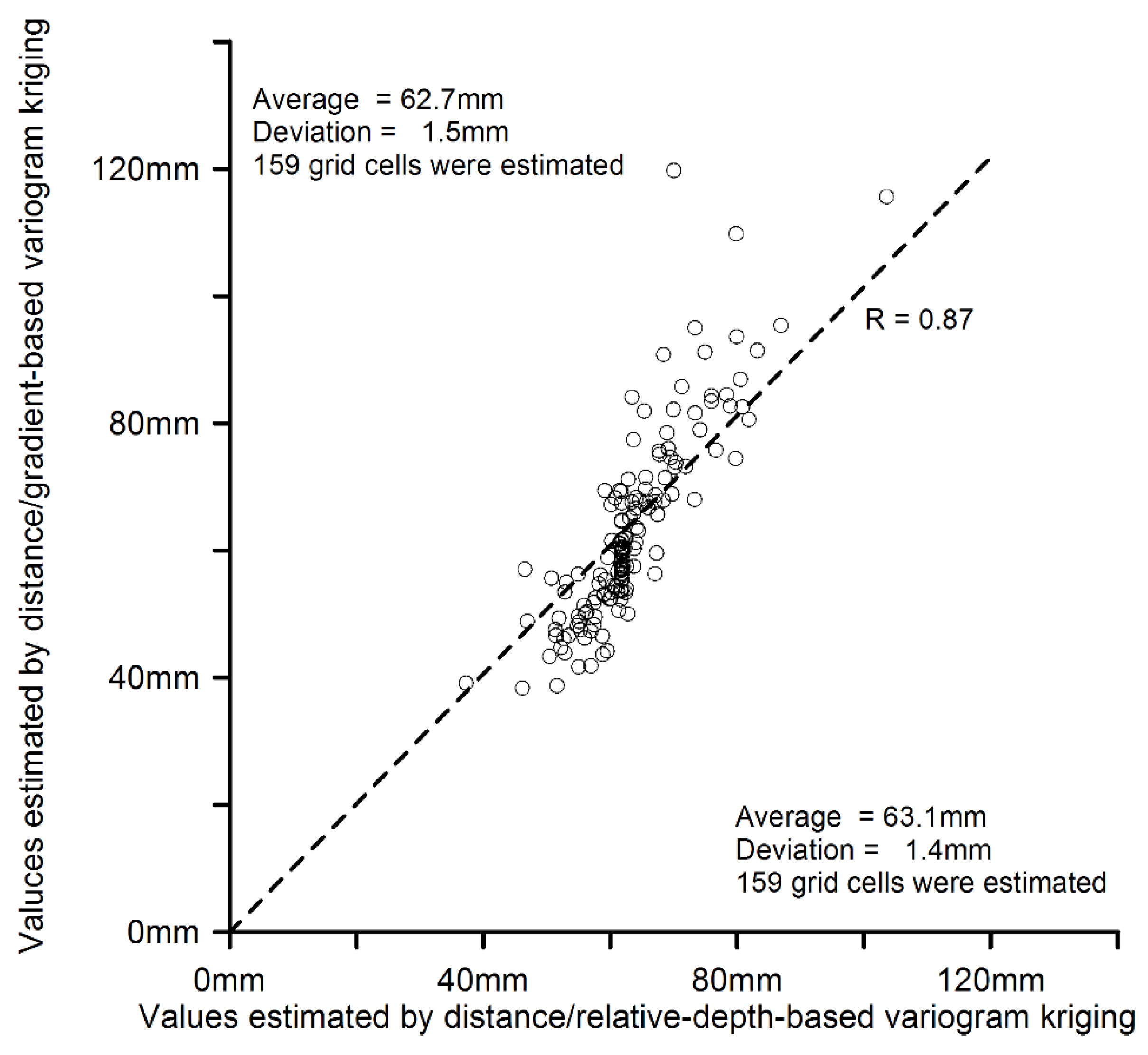
5.3. Kriging Compared with the Distance/Gradient-Based Variogram Kriging on 159 Grid Cells

169 grid cells were interpolated when distance/relative-depth-based variogram kriging was used, whereas 182 grid cells were interpolated when distance/gradient-based variogram kriging was used. From among these grid cells, 159 grid cells exhibit two values that can be estimated by the two aforementioned kriging methods. By comparing the two values obtained from 159 grid cells in Figure 10, we can infer that the interpolation effects of the aforementioned kriging methods were similar even though the deviation was smaller when distance/relative-depth-based variogram kriging was used.

6. Conclusions

Here, we presented an alternative tool to the distance/gradient-based variogram (i.e., the distance/relative-depth-based variogram). The distribution of cobalt-rich crust thicknesses estimated using this alternative variogram was coherent with that estimated using the distance/gradient-based one, and it was more convenient and easier.

The application example of the Magellan seamounts demonstrated that both distance/depth-based variograms can play an important role in expressing the spatial continuity of cobalt-rich crusts on seamounts. The distribution of the survey stations on single seamounts is often too sparse to allow variogram fitting; however, data from several adjacent seamounts with similar distribution characteristics for cobalt-rich crust thicknesses can be unified to obtain a sufficient dataset for variogram application and fitting. The variogram obtained using such data can be applied to a single seamount using the proposed kriging interpolation method.

As a component of our geostatistical scheme, it was proven that the kriging interpolation method can improve the interpolation results compared with nongeostatistical interpolation methods. Since the survey samples are expensive to obtain and the location data regarding seamounts are sparse, our approach may play an important role in evaluating cobalt-rich crusts on seamounts.

The ranges in different slope gradients could provide reference data for the design of sampling sites when surveying seamounts. Our results suggest that the spacing of these sampling sites should be smaller than the given ranges (i.e., 6000–12,000 m for bathymetric contour orientations and 2000–4000 m for gradient orientations). Our method could be effectively used not only for guyots but also for steeple top seamounts and mountain slopes on land. Moreover, it could be used to determine not only cobalt-rich crust thicknesses but also other parameter values, such as crustal element concentrations. We plan to study these aspects in the future.

The spatial continuity of cobalt-rich crusts on seamount slopes was found to form the basis for spatial interpolation. At some locations, this continuity may be destroyed by natural mechanical processes. Therefore, when interpolating for mineral resource evaluation using the kriging interpolation or similar methods, it is important to take into account a variety of factors (e.g., the slope stability and the sediment cover history).

References

- Hein, J.R. Cobalt-rich ferromanganese crusts: Global distribution, composition, origin and research activities. In Minerals Other than Polymetallic Nodules of the International Seabed Area, Proceedings of the International Seabed Authority Workshop, Kingston, Jamaica, 26–30 June 2000; International Seabed Authority: Kingston, Jamaica, 2002; Volume 2, pp. 36–89. Available online: https://www.researchgate.net/publication/264382918 (accessed on 29 August 2018).
- Hein, J.R.; Koschinsky, A.; Bau, M.; Manheim, F.T.; Kang, J.K. Cobalt-rich ferromanganese crusts in the Pacific. In Handbook of Marine Mineral Deposits, 1st ed.; Cronan, D.S., Ed.; CRC Press: Boca Raton, FL, USA, 1999; Volume 2, pp. 239–279. Available online: https://www.researchgate.net/publication/264383136 (accessed on 29 August 2018).
- Verlaan, P.A.; Cronan, D.S.; Morgan, C.L. A comparative analysis of compositional variations in and between marine ferromanganese nodules and crusts in the South Pacific and their environmental controls. Prog. Oceanograp. 2004, 63, 125–158. [Google Scholar] [CrossRef]
- Carr, J.R. Geostatistics for natural resources evaluation. Environ. Eng. Geosci. 1998, 4, 278–279. [Google Scholar] [CrossRef]
- Matheron, G. La Theorie Des Variables Regionaliseesetses Applications; Ecole Nat. Sup. Des Mines: Paris, France, 1971. [Google Scholar]
- Journel, A.G.; Huijbregts, C.J. Mining Geostatistics; Academic Press: London, UK, 1978. [Google Scholar]
- Usui, A.; Someya, M. Distribution and composition of marine hydrogenetic and hydrothermal manganese deposits in the Northwest Pacific. Geol. Soc. Lond. Spec. Publ. 1997, 119, 177–198. [Google Scholar] [CrossRef]
- Zhang, F.Y.; Zhang, W.; Zhu, K.; Zhang, X.; Zhu, B. Distribution characteristics of cobalt-rich ferromanganese crust resources on submarine seamounts in the Western Pacific. Acta Geol. Sin. 2008, 82, 796–803. [Google Scholar]
- Armstrong, M. Improving the Estimation and Modelling of the Variogram. In Geostatistics for Natural Resources Characterization; Springer: Dordrecht, The Netherlands, 1984. [Google Scholar]
- Cressie, N.A. Statistics for Spatial Data; Wiley: New York, NY, USA, 1993. [Google Scholar]
- Cressie, N.; Hawkins, D.M. Robust estimation of the variogram: I. J. Int. Assoc. Math. Geol. 1980, 12, 115–125. [Google Scholar] [CrossRef]
- Isaaks, E.H.; Srivastava, R.M. Spatial continuity measures for probabilistic and deterministic geostatistics. Math. Geol. 1988, 20, 313–341. [Google Scholar] [CrossRef]
- Isaaks, E.H.; Srivastava, R.M. An Introduction to Applied Geostatistics; Oxford University Press: New York, NY, USA, 1989; pp. 483–485. [Google Scholar]
- Journel, A.G. Geostatistics for the Environmental Sciences: An Introduction; US Environmental Protection Agency, Environmental Monitoring Systems Laboratory: Washington, DC, USA, 1987.
- Journel, A.G. New distance measures: The route toward truly nongaussian geostatistics. Math. Geol. 1988, 20, 459–475. [Google Scholar] [CrossRef]
- Omre, H. The variogram and its estimation. In Geostatistics for Natural Resources Characterization; Springer: Dordrecht, The Netherlands, 1984; pp. 107–125. [Google Scholar] [CrossRef]
- Du, D.; Wang, C.; Du, X.; Yan, S.; Ren, X.; Shi, X.; Hein, J.R. Distance-gradient-based variogram and kriging to evaluate cobalt-rich crust deposits on seamounts. Ore Geol. Rev. 2017, 84, 218–227. [Google Scholar] [CrossRef]
- Hein, J.R.; Conrad, T.A.; Dunham, R.E. Seamount characteristics and mine-site model applied to exploration and mining-lease-block selection for cobalt-rich ferromanganese crusts. Mar. Geores. Geotechnol. 2009, 27, 160–176. [Google Scholar] [CrossRef]
- Du, D.; Ren, X.; Yan, S.; Shi, X.; Liu, Y.; He, G. An integrated method for the quantitative evaluation of mineral resources of cobalt-rich crusts on seamounts. Ore Geol. Rev. 2017, 84, 174–184. [Google Scholar] [CrossRef]
- Gousie, M.B.; Franklin, W.R. Converting Elevation Contours to a Grid; Dept of Geography Simon Fraser University: Burnaby, BC, Canada, 1998; pp. 647–656. Available online: https://www.researchgate.net/profile/Michael_Gousie/publication/2318287_Converting_Elevation_Contours_to_a_Grid/links/0deec52cb05f8df45f000000.pdf (accessed on 29 August 2018).
- Jean-Laurent, M. Book Review: Geomodeling, Mathematical Geology; Springer: Berlin, Germany, 2004; Volume 36, pp. 283–286. Available online: https://link.springer.com/article/10.1023%2FB%3AMATG.0000020673.98166.ea (accessed on 29 August 2018).
- Deutsch, C.V.; Wang, L. Quantifying object-based stochastic modeling of fluvial reservoir. Math. Geol. 1996, 28, 857–880. [Google Scholar] [CrossRef]
- Deutsch, C.V.; Journel, A.G. GSLIB Geostatistical Software Library and User’s Guide; Oxford University Press: New York, NY, USA, 1998. [Google Scholar]
- Gendzwill, D.J.; Stauffer, M.R. Analysis of triaxial ellipsoids: Their shapes, plane sections, and plane projections. J. Int. Assoc. Math. Geol. 1981, 13, 135–152. [Google Scholar] [CrossRef]
© 2018 by the authors. Licensee MDPI, Basel, Switzerland. This article is an open access article distributed under the terms and conditions of the Creative Commons Attribution (CC BY) license (http://creativecommons.org/licenses/by/4.0/).