The Process of the Intensification of Coal Fly Ash Flotation Using a Stirred Tank

Abstract

Pulp preconditioning using a stirred tank as a pretreatment process is vital to the flotation system, which can be used to improve the flotation efficiency of mineral particles. The kinetic energy that is dissipated in the stirred tank could strengthen the interaction process between mineral particles and flotation reagents to improve the flotation efficiency in the presence of the preconditioning. In this paper, the effect of the conditioning speed on the coal fly ash flotation was investigated using numerical simulations and conditioning-flotation tests. The large eddy simulation coupled with the Smagorinsky-Lilly subgrid model was employed to simulate the turbulence flow field in the stirred tank, which was equipped with a six blade Rushton turbine. The impeller rotation was modelled using the sliding mesh. The simulation results showed that the large eddy simulation (LES) well matched the previous experimental data. The turbulence characteristics, such as the mean velocity, turbulent kinetic energy, power consumption and instantaneous structures of trailing vortices were analysed in detail. The turbulent length scale (η) decreased as the rotation speed increased, and the minimum value of η was almost unchanged when the rotation speed was more than 1200 rpm. The conditioning-flotation tests of coal fly ash were conducted using different conditioning speeds. The results showed that the removal of unburned carbon was greatly improved due to the strengthened turbulence in the stirred tank, and the optimal results were obtained with an LOI of 3.32%, a yield of 78.69% and an RUC of 80.89% when the conditioning speed was 1200 rpm.

1. Introduction

Coal is the main energy source in China [1]. However, the direct combustion of coal in thermal power plants has released many pollutants into the environment [2]. Coal fly ash (FA) is one of the main by-products of pulverized coal combustion [3]. The unburned carbon (UC) content in FA, which is evaluated using conventional loss on ignition (LOI), might be an obstacle for the utilization of FA in a variety of industries, especially for its use as a raw material in cement and concrete [4]. The recommended LOIs of the Class 1 and 2 fly ash types used in concrete should be less than 5% and 8%, respectively, according to the GB/T 1596-2017 [5]. The UC collected from FA could be used as activated carbon materials, graphite-like materials, etc. [6,7]. Froth flotation is still the main method for the separation of unburned carbon from FA [8,9].

Froth flotation is an important beneficiation method to realize the separation of valuable minerals and gangue minerals. The essence of flotation preconditioning is the flow-transfer-adsorption(reaction) process with multiple components, multiple scales and three phases, where the process factor determines the flotation efficiency and ability. Currently, the research on the physicochemical characteristics on the interface of mineral-reagents and mineral-bubbles has achieved good results [10,11], while the process intensification mechanism caused by the fluid strengthening lacks in-depth study. Pulp conditioning as a pretreatment before the flotation operation is of great importance to the flotation system [12,13]. Feng et al. studied the effect of conditioning methods on the flotation of nickel ore and found that high intensity conditioning could increase pentlandite flotation recovery significantly compared with the addition of Calgon [14]. Yu et al. investigated the effect of agitation on the interaction of coal and kaolinite during flotation and found that mild agitation (0~1200 rpm) could enhance the kaolinite-coating, which would lead to lower combustible matter recovery, while high intensity agitation (1200–2000 rpm) mitigated the kaolinite-coating [15]. Tabosa and Rubio investigated copper sulphide flotation assisted by high intensity conditioning and the results showed that the high intensity conditioning, as a pre-flotation stage, could increase both the copper grade and recovery [16].

Stirred tanks always play an important role in flotation preconditioning [17]. The flow structure in stirred tanks is three-dimensional, complex and has high shear. The computational fluid dynamics (CFD) simulation is used to promote the study of the fundamental phenomena, which could provide the flow field information in the stirred tank [18]. As we know, the large eddy simulation (LES) could obtain the precision flow field information, and its computational consumption is between the direct numerical simulation (DNS) and the Reynolds-averaged Navier-Stokes equations (RANS) [19]. Large eddy simulation was first applied in the simulation of stirred tanks by Eggles and was proven to be a good method to study turbulent flows [20]. The basic idea of large eddy simulations is filtering. The turbulent movement could be decomposed into the resolved scales (which include the larger scale fluctuations) and the unresolved scales (which include all the smaller scale fluctuations) through filtration. The turbulent movement of the resolved scale could be solved directly using the numerical calculation method. However, for the unresolved scale, the effects of the mass, momentum and energy transport on the larger scale movement are modelled using a subgrid-scale model, which can closely approximate the movement equation [21].

The turbulence flow in the stirred tank can be regarded as the formation of turbulent vortexes, which is the main driving force for fluid shear, dispersion and uniform mixing. The interaction process between particles and reagents is completed in the full turbulent flow field of the stirred tank since the turbulence has an important role in the interaction process. The turbulent fluctuations in the turbulence movement could be regarded as the simultaneous existence of energetic vortices with different length scales. The energetic vortices possess the vast majority of the fluid kinetic energy and pass the energy to the smaller vortices step by step. The energy input agitated by the impeller rotation is dissipated by the heat transfer due to the molecular viscosity of the fluid at the smallest vortices in the stirred tank. The smallest scale of energy dissipation of the turbulent vortices is also called the turbulent microscale (η). The kinetic energy that is dissipated in the stirred tank could strengthen the interaction process between the mineral particles and the flotation reagents to improve the flotation efficiency in the presence of preconditioning with a stirred tank.

It was validated that the hydrodynamic conditions had important influences on the breakup of droplets breakup [22], the particle agglomeration in crystallizers [23], the micromixing [24] and the passive scalar transport [25] in the processing performance. This paper focuses on the turbulent properties in the outflow generated by the Rushton turbine in a stirred tank and the conditioning-flotation tests of the flotation separation of unburned carbon from coal fly ash. The simulation results were compared with previous studies to validate the reliability of the large eddy simulation (LES). The trailing vortices and the turbulence length scale under different conditioning speeds were investigated. Then, conditioning-flotation tests were carried out to verify the optimal turbulence flow field with the purpose to improve the separation efficiency of unburned carbon from coal fly ash.

2. Methodology

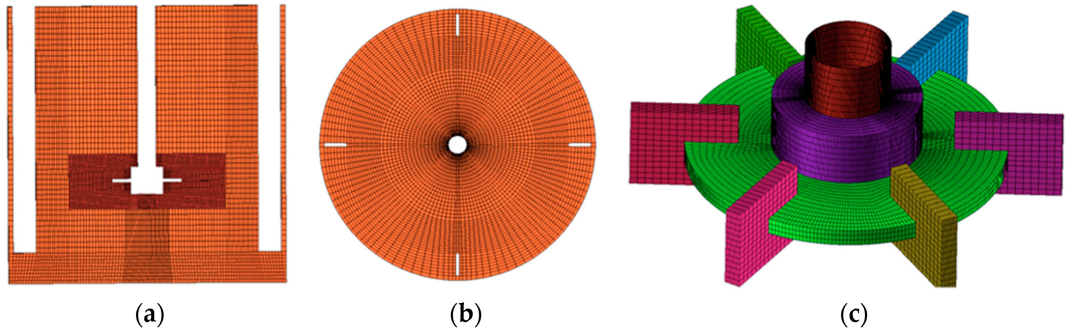
2.1. Geometry Structure

The stirred tank was a standard cylindrical vessel of diameter T = 300 mm, which was stirred by a six blade Rushton turbine, was equipped with four equi-spaced baffles of width 1/12 T and had a liquid height of H = T, as shown in Figure 1. The impeller had a diameter of D = T/3 and a clearance of C = T/3. The working fluid was water with a density of 1000 kg/m³ and a kinematics viscosity of 1.006 × 10⁻⁶ m²/s. The impeller rotational speeds were 300, 600, 900, 1200, and 1500 rpm, the Reynolds number ($R_e=N{D}^2/v$, $v$ is the fluid kinematics viscosity and N is the impeller rotational speed) was 5.0 × 10⁴ ~2.5 × 10⁵, and the impeller tip speed was $U_{tip}=\pi DN$.

2.2. Governing Equations

The LES can resolve the larger scale movements and model the smaller scale movements by employing a spatial filter for the governance of the Navier-Stokes equations. The governing equations of LES are as follows:

$$\frac{\partial {\overline{u}}_i}{\partial x_i}=0$$

(1)

$$\frac{\partial \left({\overline{u}}_i\right)}{\partial t}+{\overline{u}}_i\frac{\partial \left({\overline{u}}_j\right)}{\partial x_i}+\frac{\partial \overline{P}}{\partial x_i}=v\frac{{\partial }^2{\overline{u}}_i}{\partial x_j^2}-\frac{\partial {\tau }_{ij}}{\partial x_j}$$

(2)

$${\tau }_{ij}=\overline{u_i{u}_j}-{\overline{u}}_i{\overline{u}}_j$$

(3)

where ${\tau }_{ij}$ is the sub-grid scale stress tensor, which reflects the effect of the unresolved scale on the resolved scale [26]. In this study, the effect of the sub-grid scale on the larger scale was assessed using the Smagorinsky-Lilly model, and the eddy viscosity is modelled as $v_t=L_s^2\left|\overline{s}\right|$, where $L_s=\min \left(Kd,C_S{V}^{1/3}\right)$, $K$ is the mixing length for the subgrid scale, $d$ is the distance to the closest wall, $V$ is the volume of the computational cells, $C_S$ is the Smagorinsky constant of 0.1 in this work [27,28,29], and $\left|\overline{s}\right|=\sqrt{2{\overline{s}}_{ij}{\overline{s}}_{ij}}$, ${\overline{s}}_{ij}$ is the rate of the strain tensor for the resolved scale.

2.3. Numerical Methods

The numerical simulations were conducted using the FLUENT software. A fine mesh with a high quality and a small time step should be used in the LES. The computational meshes were divided into two parts: a rotation cylindrical volume that included the impeller, and a stationary part that contained the rest of the tank. The computational meshes with homogeneous hexahedral structure were generated by the ICEM. A mesh independence test was carried out at the rotation speed of 300 rpm. The volume-averaged turbulence dissipation rate was chosen as the principle criterion of the mesh quality [30] and the results are shown in Figure 2. The figure shows that the volume-averaged turbulence dissipation rate had a slight change when the mesh quantity was larger than 0.86 million, and so the mesh quantity of 0.86 million was chosen for the numerical calculation at 300 rpm. On this basis, considering the computational demand, the mesh quantity, mainly in the vicinity of the impeller, was increased to approximately 1.20 million, 1.61 million, 2.21 million and 3.16 million for the numerical calculations at 600 rpm, 900 rpm, 1200 rpm and 1500 rpm, respectively. The mesh schematics at the rotation speed of 300 rpm are shown in Figure 3.

The LES with the Smagorinsky-Lilly subgrid model was employed to simulate the flow field in the stirred tank. Sliding mesh (SM) was used to deal with the movement of the impeller. The complete stabilized flow field, which was obtained from the k-epsilon simulation, was used as the initial values of the LES. The second order and the bounded central differences were chosen as the spatial discretization of the pressure and momentum, respectively. The time steps used in the simulations were set at 0.001 for 300 rpm, 0.001 for 600 rpm, 0.0005 for 900 rpm, 0.0001 for 1200 rpm, and 0.0001 for 1500 rpm, which take into account the computational consumption. The total simulation time was 10 s at the agitation rates of 300 rpm and 600 rpm and 20 revolutions of the impeller for the other higher agitation rates for getting the steady flow field. Then, the flow data were collected and postprocessed. Most results stated here were the data for 300 rpm, except for special instructions.

2.4. The Post-Processing of the LES Results

Since LES solves an instantaneous velocity field, post-processing was performed to extract the mean velocity, the periodic velocity fluctuations and the turbulent velocity fluctuations according to their statistical averages using the MATLAB software. The velocity fluctuations in a turbulently stirred tank are partly periodic (or organized) and partly random (turbulent). The local instantaneous velocity $u_i$ should be decomposed into the mean, the periodic and resolved the part of the fluctuations as follows:

$$u_i=\overline{U_i}+\widetilde{u_i}+u_i^{\prime }$$

(4)

As a result, the kinetic energy can be divided into the periodic and the turbulent kinetic energy. The total kinetic energy, k_tot, in the velocity fluctuations is as follows:

$$k_{tot}=k_P+k_T$$

(5)

where $k_P$ and $k_T$ are the periodic kinetic energy and turbulent kinetic energy with respect to the total turbulent kinetic energy $k_{tot}$, respectively. The turbulent kinetic energy is calculated as follows:

$$k_T=\frac{1}{2}{\displaystyle \sum }_{i=1}^3\langle u_i^{\prime }{u}_i^{\prime }\rangle$$

(6)

The dissipation rate of the turbulent kinetic energy can be calculated from the measurements of the turbulent velocity gradients in three directions as follows:

$$\epsilon =v{S}_{ij}{S}_{ij}=\frac{v}{2}{(\frac{\partial u_i}{\partial x_j}+\frac{\partial u_j}{\partial x_x})}^2$$

(7)

3. Numerical Simulation Results and Discussion

3.1. Mean Velocity

The mean velocity of the LES results in a radial position of r/R = 1.07 in the impeller jet flow, which is normalized by the impeller tip velocity (U_tip), as shown in Figure 4. Figure 4 shows the comparison results between the simulations and previous experiments (LDV data from Wu, 1989 [31]; and PIV data from Escudié, 2001 [32]). 2z/W = 0 represented the central position of the impeller disc, and Ur, Ut and Uz represented the radial velocity, tangential velocity and axial velocity, respectively. The radial velocity of the LES agreed well with the previous experiments. For the simulation results and previous experiments, they have almost the same width of the flow entrainment area, and the peak location of the radial velocity was at 2z/W = 0. For the tangential velocity, the value of the peak in the simulation was slightly higher, while the location was in better agreement with the LDV results and slightly lower compared with the PIV results. In addition, a wider flow entrainment area was obtained compared with the experimental results. The axial velocity was evidently smaller than the radial velocity and the tangential velocity, and it was almost zero around the central position, which was because the fluid split into two streams in opposite directions. It could be seen that there was a difference between the velocity of the simulations and experiments at both ends of the jet flow area. The fine distinction of the mean velocity might be caused by the geometrical shape, experimental methods and operating conditions [33,34,35].

3.2. Turbulent Kinetic Energy

The dimensionless turbulent kinetic energy (k_T/U_tip²) at the radial position of r/R = 1.07 was compared with the previous work (the PIV data from Escudié, 2001 [32]) to validate the LES under all rotation speeds, as shown in Figure 5. The turbulent kinetic energy was larger in the vicinity of the impeller, and it decreased as it moved away from the impeller. The upper impeller outflow was slightly larger than the lower impeller outflow in the simulations for all the rotation speeds. The width of the peaks of the LES simulations and PIV data were roughly aligned. It can be seen that a good agreement was found for the simulation results and PIV data. There was also a difference between the LES results and the previous experimental data, which may be due to the insufficient spatial resolution of the mesh size and the difference in the geometrical shapes [36,37].

3.3. Flow Rate Balance

The radial and axial flow rates through the control surfaces can be expressed as follows:

$$Q_r=2\mathsf{\pi }r{{\displaystyle \int }}_{z_1}^{z_2}{U}_{r}dz$$

(8)

where $z_1$ = −20 mm, $z_2$ = 20 mm, r₁ = 0 or 55 mm, and r₂ = 55 or 85 mm. The radial pumping flow rate of the impeller ($Q_r$) is defined as the integral of the average radial velocity component over the entire impeller stream.

Table 1. Flow rate balance around the impeller at 300 rpm, −20 ≤ z ≤ 20 (mm).

Region	Flow in (L/s)	Flow out (L/s)	Difference (%)
0 ≤ r ≤ 55 mm	0.3683	0.3735	1.4
55 ≤ r ≤ 85 mm	0.7474	0.7422	0.7

shows the volume flow rate balance around two control volumes that contain the impeller. One of the radial regions is r = 0~55 mm, the other is r = 55~80 mm, and both of them range from $z$ = −20~20 mm. It could be seen that the differences between the flow in and flow out were within 1.5%, which proved the reliability of the simulation results [31].

3.4. Trailing Vortices behind the Blades

Figure 6 shows the iso-surface of the Q criterion (Q = 7 × 10⁴ s⁻²) behind each blade at different rotation times, which are coloured based on the velocity magnitude. The three-dimensional structure of the turbulent vortex was clear from the simulation results. The large-scale eddies embody themselves in the form of identifiable and organized distributions of the vorticity and are mainly responsible for the mixing performance [38,39]. The trailing vortices, one upper and one lower, formed at the rear of the blade and were attached to the end of the impeller disk. They unfolded along the blade outline, and then separated from the blade tip. There was a high-speed belt between the two vortices that lie in the bottom of the upper vortex and the top of the lower vortex. The fluid element is reduced by the vortex split and energy transfer to achieve small size micro mixing. The instantaneous structures of the trailing vortices accompanied by the vortex tube’s winding, kink, fracture and reattachment were generated at different evolution times. The trailing vortices are associated with high shear rates and strong turbulent activity, and therefore they are essential to the mixing performance of the flow field [40]. The continuous movement and deformation of the vortex in the turbulent flow field could accelerate the energy dissipation and the loss of the mechanical energy, which could enhance the interaction between the flotation reagents and mineral particles to improve the separation efficiency of the coal fly ash flotation with the pulp preconditioning.

3.5. Power Consumption under Different Rotation Speeds

The numerical simulation model used in this paper was able to predict the power consumption of the stirred tank. The power consumption (P) was calculated from the equation P = 2πMN, where M is the torque of the impeller, and N is the impellor’s rotation speed [41]. The power number Np ($N_P=\frac{P}{\rho N^3{D}^5}$, where $\rho$ is the density of water and D is the impeller diameter) was used to check the validity of the LES model used in the simulation [42]. The power consumption and power number of the impeller under different rotation speeds are shown in Figure 7. The power consumption increased with the rotation speed, while the power number had a slight change. The power consumption had a large growth trend as it varied from 5.86 W to 736.06 W when the rotation speed changed from 300 rpm to 1500 rpm. Hudcova et al. also studied the influence of flow patterns on the power consumption and flow regime transition in a gas-liquid stirred vessel [43]. The average Np of the simulation results was found to be approximately constant at 4.65 for all the Reynolds numbers at the tested range, which was logical in comparison with that reported by Zadghaffari et al. of Np = 4.8 for six Rushton turbines [34]. Np represents the effective transmission of the energy to the processed liquid by the impellers [44].

3.6. Turbulent Length Scale

The energy input agitated by the impeller rotation that dissipated into the stirred tank could accelerate the interaction between the mineral particles and flotation reagents. The smallest turbulent microscale of the energy dissipation of the energetic vortices is also called the Kolmogorov scale (η), which can be estimated by the dissipation rate of the turbulent kinetic energy, and can be expressed as

$$\eta ={\left(\frac{v^3}{ϵ}\right)}^{1/4}$$

(9)

where $v$ is the kinematic viscosity and $ϵ$ is the dissipation rate of the turbulent kinetic energy. Most turbulent kinetic energy is consumed by the viscosity of the smallest eddy [45].

The Kolmogorov scale (η) at the position of r/R = 1.07 and −2 < 2z/w < 2 under different rotation speeds is plotted in Figure 8. Figure 8 shows that η decreases as the rotation speed increases. The Kolmogorov scale ranged from 11 μm to 87 μm in the jet flow when the rotation speed was 300 rpm, and then it narrowed to 3~46 μm at 1200 rpm and 3~38 μm at 1500 rpm. This magnitude is consistent with those previously reported [46,47]. The minimum Kolmogorov scale under the tested rotation speeds was approximately 3 μm, and it remained mostly unchanged when the rotation speed was beyond 1200 rpm. The energy that dissipated into the stirred tank could strengthen the interaction process between particles and reagents and improve the separation efficiency of the coal fly ash flotation.

4. Conditioning-Flotation Experiments

4.1. Materials and Methods

The coal fly ash samples were collected from a thermal power plant in Hunan, China. The particle size analysis according to the wet screening showed that −0.045 mm was the dominant size fraction with a yield of 50.72%, a loss on ignition of 12.14% and a carbon distribution of 48.40%. This showed that the flotation efficiency of fine particles was crucial in the separation of unburned carbon from coal fly ash. The contact angle of the fly ash sample was measured using an optical contact angle analysis system (DSA100, Krüss, Germany). It decreased quickly with the increase of the measurement time and was almost 0° at 2 s, as shown in Figure 9, which implied poor floatability of fly ash [48,49,50]. Light diesel oil and a 730-flotation reagent (prepared by mixing polyethylene glycol and 2-octanol at an appropriate ratio) were used as the collector and frother, respectively.

Stirred tanks are widely used for pulp preconditioning processing. Stirred tank was a standard cylindrical vessel, and the geometric dimensions were the same as those in the simulation (Figure 1). For the preconditioning tests, the height of the working fluid was equal to the diameter of the stirred tank. Then, the FA samples and collector were added into the stirred tank with a concentration of approximately 100 g/L and a dosage of 1000 g/t, respectively. The conditioning speeds were set as 300 rpm, 600 rpm, 900 rpm, 1200 rpm, and 1500 rpm at the conditioning time of 5 min (according to the preliminary tests). The pulp of 1 L was collected and prepared for the following flotation tests.

The flotation tests were carried out with a 1.0 L XFD lab-scale single flotation cell at an impeller speed of 1600 rpm. Then, the frother was added to the slurry and stirred for 1 min. Subsequently, the air with a flow rate of 1.67 L/min was introduced into the flotation cell. The total flotation time was 4 min. The collected concentrates and tailings were filtered, dried, and weighed for the following analysis.

The muffle furnace combustion method is used to measure the loss on ignition (LOI) of the concentrates and the tailings product [8,51]. The LOI is calculated as

$$\mathrm{LOI}(\%)=\frac{W_b-W_a}{W_b}\times 100$$

(10)

where $W_b$ and $W_a$ are the weight of the samples before burning and after burning, respectively.

The removal rate of unburned carbon (RUC) in the tailings is equal to the recovery rate of unburned carbon in the concentrates for the flotation tests and is computed a

$$\mathrm{RUC}(\%)=\frac{LO{I}_C\times Y_C}{LO{I}_R}\times 100$$

(11)

where $LO{I}_C$ and $Y_C$ are the LOI and yield of the concentrates, respectively, and $LO{I}_R$ is the LOI of the raw fly ash.

4.2. Experimental Results and Discussion

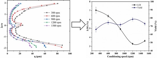
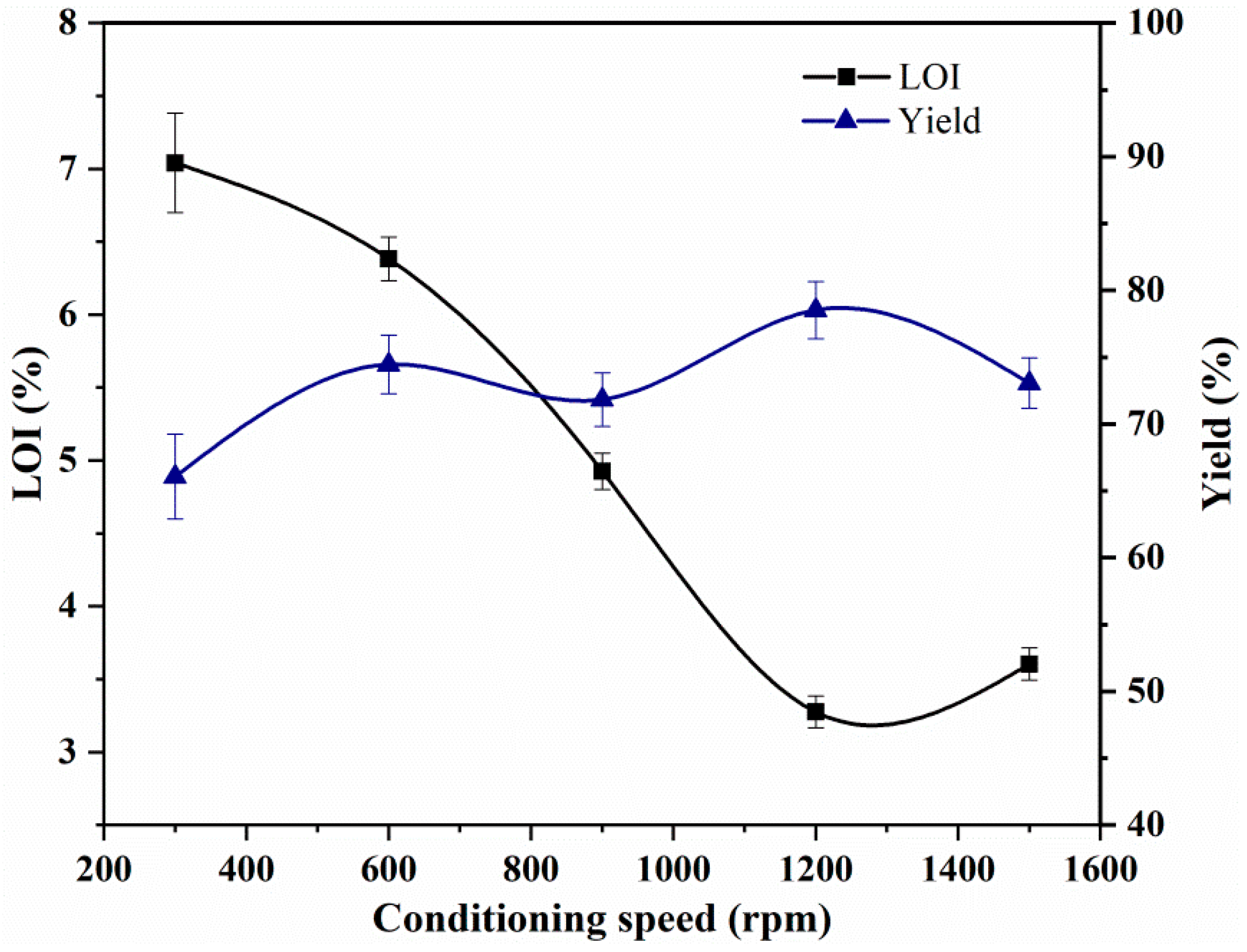
4.2.1. Effect of the Conditioning Speed on the LOI and Yield of Flotation Tailings

The pulp preconditioning before flotation processing could promote the flotation behaviour of fine mineral particles. The effects of the condition speed on the LOI and the yield of the flotation tailings are shown in Figure 10. The LOI decreased as the conditioning speed increased. Then, it had a slight increase while the yield had a slight change. The yield of the flotation tailing ash varied from 66.87% to 78.69% at the tested range (300 rpm~1500 rpm). The LOI of the trailing ash decreased from 7.06% to 3.32% as the LOI of the feed coal fly ash samples was 12.72% when the conditioning speed increased from 300 rpm to 1200 rpm. The flotation tailing products, which had a lower LOI (less than 8%), could be used in the concrete according to the national standard GB/T 1596-2017. The probability of collision and attachment between the mineral particles and the flotation reagent increased with the turbulence fluctuation, which was caused by the increase of the conditioning speed, while the excessive fluctuation frequency would increase the possibility of detachment. Deglon concluded that increasing the level of agitation generally has a beneficial effect on the flotation rate of platinum ores [52].

4.2.2. Effect of the Conditioning Speed on the RUC of Flotation Concentrates

Figure 11 shows the effect of the conditioning speed on the recovery rate of unburned carbon (RUC) in the conditioning-flotation tests. It can be seen that the RUC under the tested conditioning speeds first increases and then decreases with the increase of the conditioning speed. The RUC reached the maximum of 80.89% at the conditioning speed of 1200 rpm. The UC collected from the FA could be used as some industrial materials or fed back to the boiler as fuel energy [53]. The optimal conditioning-flotation results were obtained with an LOI of 3.32%, a yield of 78.69% and an RUC of 80.89% when the conditioning speed was 1200 rpm. This was consistent with the LES results that the smallest turbulent scale (η) was obtained at the rotation speed of 1200 rpm, and the energy that dissipated into the stirred tank would not increase when the rotation speed exceeded 1200 rpm. Many authors claimed that energy transferred in the conditioning stage had a pronounced effect on the concentrate recovery, grade and flotation rate [16]. The preconditioning process with the energy input by the stirred tank could strengthen the interaction process between the particles and reagents, while the excessive energy input could not improve the flotation efficiency. The conditioning-flotation tests revealed the effect of the turbulence hydrodynamics due to the impeller rotation on the intensification of the coal fly ash flotation in the presented of preconditioning with a stirred tank.

5. Conclusions

The pulp preconditioning using a stirred tank is important to strengthen the separation efficiency of coal fly ash in the flotation process. The turbulence characteristics and the turbulence length scale under different rotation speeds in the stirred tank were studied using large eddy simulation (LES). The conditioning-flotation tests were carried out to valid the effect of the turbulence flow field on the flotation strengthening by investigating the effect of the conditioning speed on the removal of unburned carbon from coal fly ash. The main conclusions are as follows.

The LES results were in good agreement with the previous experimental data. The turbulent kinetic energy, power consumption and instantaneous structure of trailing vortices at different evolution times were investigated in detail.

The turbulence length scale (η) decreased as the rotation speed increased and the minimum value of η was approximately 3 μm, and it remained mostly unchanged when the rotation speed exceeded 1200 rpm. The turbulent kinetic energy that dissipated into the stirred tank dominate the process of the intensification in stirred tank.

The conditioning-flotation tests showed that the optimal results were obtained with an LOI of 3.32%, a yield of 78.69% and an RUC of 80.89% at the conditioning speed of 1200 rpm. This was consistent with the simulation results, which showed the process strengthening effect of the turbulence hydrodynamics in the stirred tank on the flotation separation of unburned carbon from coal fly ash.

References

1. Xu, Z.; Liu, J.; Choung, J.W.; Zhou, Z. Electrokinetic study of clay interactions with coal in flotation. In. J. Miner. Process. 2003, 68, 183–196. [Google Scholar] [CrossRef]
2. Hartuti, S.; Hanum, F.F.; Takeyama, A.; Kambara, S. Effect of Additives on Arsenic, Boron and Selenium Leaching from Coal Fly Ash. Minerals 2017, 7, 99. [Google Scholar] [CrossRef]
3. Li, S.; Wu, W.; Li, H.; Hou, X. The direct adsorption of low concentration gallium from fly ash. Sep. Technol. 2016, 51, 395–402. [Google Scholar] [CrossRef]
4. ASTM D7348-13, Standard Test Methods for Loss on Ignition (LOI) of Solid Combustion Residues; ASTM International: West Conshohocken, PA, USA, 2013.
5. Fly Ash Used for Cement and Concrete; PRC National Standard; Standardization Administration of the People’s Republic of China: Beijing, China, 2017; GB/T 1596-2017.
6. Bartoňová, L. Unburned carbon from coal combustion ash: An overview. Fuel Process. Technol. 2015, 134, 136–158. [Google Scholar] [CrossRef]
7. Cameán, I.; Garcia, A.B. Graphite materials prepared by HTT of unburned carbon from coal combustion fly ashes: Performance as anodes in lithium-ion batteries. J. Power Sources 2011, 196, 4816–4820. [Google Scholar] [CrossRef]
8. Cao, Y.; Li, G.; Liu, J.; Zhang, H.; Zhai, X. Removal of unburned carbon from fly ash using a cyclonic-static microbubble flotation column. J. S. Afr. I. Min. Metall. 2012, 112, 891–896. [Google Scholar]
9. An, M.; Liao, Y.; Zhao, Y.; Li, X.; Lai, Q.; Liu, Z.; He, Y. Effect of frothers on removal of unburned carbon from coal-fired power plant fly ash by froth flotation. Sep. Sci. Technol. 2018, 53, 535–543. [Google Scholar] [CrossRef]
10. Peng, Y.; Grano, S. Effect of iron contamination from grinding media on the flotation of sulphide minerals of different particle size. Int. J. Miner. Process. 2010, 97, 1–6. [Google Scholar] [CrossRef]
11. Piñeres, J.; Barraza, J. Energy barrier of aggregates coal particle-bubble through the extended DLVO theory. Int. J. Miner. Process. 2011, 93, 14–20. [Google Scholar] [CrossRef]
12. Hao, J.; Gao, Y.; Khoso, S.; Ji, W.Y.; Hu, Y.H. Interpretation of Hydrophobization Behavior of Dodecylamine on Muscovite and Talc Surface through Dynamic Wettability and AFM Analysis. Minerals 2018, 8, 391. [Google Scholar]
13. Sun, W.; Xie, Z.J.; Hu, Y.H.; Deng, M.J.; Yi, L.; He, G.Y. Effect of high intensity conditioning on aggregate size of fine sphalerite. T. Nonferr. Metals. Soc. 2008, 18, 438–443. [Google Scholar] [CrossRef]
14. Feng, B.; Feng, Q.M.; Lu, Y.P. The effect of conditioning methods and chain length of xanthate on the flotation of a nickel ore. Miner. Eng. 2012, 39, 48–50. [Google Scholar] [CrossRef]
15. Yu, Y.X.; Cheng, G.; Ma, L.Q.; Huang, G.; Wu, L.; Xu, H. Effect of agitation on the interaction of coal and kaolinite in flotation. Powder Technol. 2017, 313, 122–128. [Google Scholar] [CrossRef]
16. Tabosa, E.; Rubio, J. Flotation of copper sulphides assisted by high intensity conditioning (HIC) and concentrate recirculation. Miner. Eng. 2010, 23, 1198–1206. [Google Scholar] [CrossRef]
17. Feng, D.; Aldrch, C. Effect of preconditioning on the flotation of coal. Chem. Eng. Commun. 2005, 192, 972–983. [Google Scholar] [CrossRef]
18. Pan, A.; Xie, M.H.; Li, C.; Xia, J.Y.; Chu, J.; Zhuang, Y.P. CFD Simulation of Average and Local Gas–Liquid Flow Properties in Stirred Tank Reactors with Multiple Rushton Impellers. J. Chem. Eng. Jpn. 2017, 50, 878–891. [Google Scholar] [CrossRef] [Green Version]
19. Vlček, P.; Kysela, B.; Jirout, T.; Fořt, I. Large eddy simulation of a pitched blade impeller mixed vessel-comparison with LDA measurements. Chem. Eng. Res. Des. 2016, 108, 42–48. [Google Scholar] [CrossRef]
20. Eggels, J.G. Direct and Large-eddy Simulation of Turbulent Fluid Flow Using the Lattice-Boltzmann Scheme. Int. J. Heat Fluid 1996, 17, 307–323. [Google Scholar] [CrossRef]
21. Bakker, A.; Oshinowo, L.M. Modelling of turbulence in stirred vessels using large eddy simulation. Chem. Eng. Res. Des. 2004, 82, 1169–1178. [Google Scholar] [CrossRef]
22. Zhou, G.; Kresta, S.M. Correlation of mean drop size and minimum drop size with the turbulence energy dissipation and the flow in an agitated tank. Chem. Eng. Sci. 1998, 53, 2063–2079. [Google Scholar] [CrossRef]
23. Smoluchowski, M.V. Versuch einer mathematischen theorie der koagulations kinetis kolloider losungen. Z. Phys. Chem. 1918, 92, 129–168. [Google Scholar]
24. Bakker, R.A. Micromixing in Chemical Reactors: Models, Experiments and Simulations. Ph.D. Thesis, TU Delft, Delft, The Netherlands, 1996. [Google Scholar]
25. Yoon, H.S.; Balachandar, S.; Man, Y.H. Large eddy simulation of passive scalar transport in a stirred tank for different diffusivities. Int. J. Heat Mass Tran. 2015, 91, 885–897. [Google Scholar] [CrossRef]
26. Zadghaffari, R.; Moghaddas, J.S.; Revstedt, J. Large-eddy Simulation of Turbulent Flow in a Stirred Tank Driven by a Rushton Turbine. Comput. Fluids. 2010, 39, 1183–1190. [Google Scholar] [CrossRef]
27. Yeoh, S.L.; Papadakis, G.; Lee, K.C.; Yianneskis, M. Large Eddy Simulation of Turbulent Flow in a Rushton Impeller Stirred Reactor with Sliding-deforming Mesh Methodology. Chem. Eng. Technol. 2004, 27, 257–263. [Google Scholar] [CrossRef]
28. Min, J.; Gao, Z.M. Large Eddy Simulations of Mixing Time in a Stirred Tank. Chinese J. Chem. Eng. 2006, 14, 1–7. [Google Scholar] [CrossRef]
29. Derksen, J. Assessment of Large Eddy Simulations for Agitated Flows. Chem. Eng. Res. Des. 2001, 79, 824–830. [Google Scholar] [CrossRef] [Green Version]
30. Wang, L.; Wang, Y.; Yan, X.; Wang, A.; Cao, Y.A. Numerical study on efficient recovery of fine-grained minerals with vortex generators in pipe flow unit of a cyclonic-static micro bubble flotation column. Chem. Eng. Sci. 2017, 158, 304–313. [Google Scholar] [CrossRef]
31. Wu, H.; Patterson, G.K. Laser-Doppler Measurements of Turbulent-flow Parameters in a Stirred Mixer. Chem. Eng. Sci. 1989, 44, 2207–2221. [Google Scholar] [CrossRef]
32. Escudié, R. Structure de L’hydrodynamique Générée par une Turbine de Rushton. Ph.D. Thesis, INSA de Toulouse, Toulouse, France, 2001. (In French). [Google Scholar]
33. Jaworski, Z.; Dyster, K.N.; Nienow, A.W. The effect of size, location and pumping direction of pitched blade turbine impellers on flow patterns: LDA measurements and CFD predictions. Chem. Eng. Res. Des. 2001, 79, 887–894. [Google Scholar] [CrossRef]
34. Zadghaffari, R.; Moghaddas, J.S.; Revstedt, J. A Mixing Study in a Double-Rushton Stirred Tank. Comput. Chem. Eng. 2009, 33, 1240–1246. [Google Scholar] [CrossRef]
35. Malik, S.; Lévêque, E.; Bouaifi, M.; Gamet, L.; Ghamri, N.; Simoëns, S.; El-Hajema, M. Shear improved smagorinsky model for large eddy simulation of flow in a stirred tank with a rushton disk turbine. Chem. Eng. Res. Des. 2016, 108, 69–80. [Google Scholar] [CrossRef]
36. Zhang, Y.H.; Yang, C.; Mao, Z. Large eddy simulation of liquid flow in a stirred tank with improved inner-outer iterative algorithm. Chinese J. Chem. Eng. 2006, 14, 47–55. [Google Scholar] [CrossRef]
37. Soos, M.; Kaufmann, R.; Winteler, R.; Kroupa, M.; Lüthi, B. Determination of maximum turbulent energy dissipation rate generated by a rushton impeller through large eddy simulation. Aiche J. 2013, 59, 3642–3658. [Google Scholar] [CrossRef]
38. Bakker, A.; Oshinowo, L.M.; Marshall, E.M. Chapter 31—The Use of Large Eddy Simulation to Study Stirred Vessel Hydrodynamics. In Proceedings of the 10th European Conference, Delft, The Netherlands, 2–5 July 2000; pp. 247–254. [Google Scholar]
39. Escudié, R.; Bouyer, D.; Liné, A. Characterization of trailing vortices generated by a rushton turbine. Aiche J. 2004, 50, 75–86. [Google Scholar] [CrossRef]
40. Derksen, J.; Akker, H. Large eddy simulations on the flow driven by a rushton turbine. Aiche J. 2010, 45, 209–221. [Google Scholar] [CrossRef]
41. Deglon, D.; Meyer, C. CFD modeling of stirred tanks: Numerical considerations. Miner. Eng. 2006, 19, 1059–1068. [Google Scholar] [CrossRef]
42. Bartels, C.; Breuer, M.; Wechsler, K.; Durst, F. Computational fluid dynamics applications on parallel-vector computers: computations of stirred vessel flows. Comput. Fluids. 2002, 31, 69–97. [Google Scholar] [CrossRef]
43. Hudcova, V.; Machon, V.; Nienow, A.W. Gas-liquid dispersion with dual Rushton turbine impellers. Biotechnol. Bioeng. 1989, 34, 617–628. [Google Scholar] [CrossRef] [PubMed]
44. Taghavi, M.; Zadghaffari, R.; Moghaddas, J.; Moghaddas, Y. Experimental and cfd investigation of power consumption in a dual rushton turbine stirred tank. Chem. Eng. Res. Des. 2011, 89, 280–290. [Google Scholar] [CrossRef]
45. Escudié, R.; Liné, A. A simplified procedure to identify trailing vortices generated by a rushton turbine. Aiche J. 2010, 53, 523–526. [Google Scholar] [CrossRef]
46. Escudié, R.; Liné, A. Experimental analysis of hydrodynamics in a radially agitated tank. Aiche J. 2003, 49, 585–603. [Google Scholar] [CrossRef]
47. Yeoh, S.L.; Papadakis, G.; Yianneskis, M. Numerical simulation of turbulent flow characteristics in a stirred vessel using the les and rans approaches with the sliding/deforming mesh methodology. Chem. Eng. Res. Des. 2004, 82, 834–848. [Google Scholar] [CrossRef]
48. Dey, S. Enhancement in hydrophobicity of low rank coal by surfactants-a critical overview. Fuel Process. Technol. 2012, 94, 151–158. [Google Scholar] [CrossRef]
49. Peng, Y.; Liang, L.; Tan, J.; Sha, J.; Xie, G. Effect of flotation reagent adsorption by different ultra-fine coal particles on coal flotation. Int. J. Miner. Process. 2015, 142, 17–21. [Google Scholar] [CrossRef]
50. Xia, W.; Yang, J.; Liang, C. A short review of improvement in flotation of low rank/oxidized coals by pretreatments. Powder Technol. 2013, 237, 1–8. [Google Scholar] [CrossRef]
51. Zhou, F.; Yan, C.; Wang, H.Q.; Zhou, S.; Liang, H. The result of surfactants on froth flotation of unburned carbon from coal fly ash. Fuel 2017, 190, 182–188. [Google Scholar] [CrossRef]
52. Deglon, D.A. The effect of agitation on the flotation of platinum ores. Miner. Eng. 2005, 18, 839–844. [Google Scholar] [CrossRef]
53. Hower, J.C.; Groppo, J.G.; Graham, U.M.; Wardb, C.R.; Kostovac, I.J.; Maroto-Valer, M.M.; Dai, S.F. Coal-derived unburned carbons in fly ash: A review. Int. J. Coal Geol. 2017, 179, 11–27. [Google Scholar] [CrossRef]
Figure 1. View of (a) the stirred tank and (b) the Rushton turbine.
Minerals 08 00597 g001
Figure 2. Volume-averaged turbulence dissipation rate for different mesh quantities.
Minerals 08 00597 g002
Figure 3. View of the hexahedral mesh. (a) vertical section; (b) horizontal section; (c) impeller surface.
Minerals 08 00597 g003
Figure 4. Mean velocity normalized by Utip. (a) radial velocity; (b) tangential velocity; (c) axial velocity.
Minerals 08 00597 g004
Figure 5. The turbulent kinetic energy normalized by Utip2.
Minerals 08 00597 g005
Figure 6. The instantaneous structure of the turbulent vortices.
Minerals 08 00597 g006
Figure 7. Power consumption and power number under different rotation speeds.
Minerals 08 00597 g007
Figure 8. The Kolmogorov scale (η) under different rotation speeds.
Minerals 08 00597 g008
Figure 9. Contact angle of fly ash samples.
Minerals 08 00597 g009
Figure 10. Effect of conditioning speed on the LOI and yield of concentrates.
Minerals 08 00597 g010
Figure 11. Effect of different conditioning speeds on the RUC of the flotation tests.
Minerals 08 00597 g011