Extraction of Alteration Minerals and Prospecting Prediction in Vegetated Regions Based on GF-5B Hyperspectral Data: A Case Study of the Huzhou Region, Zhejiang Province, China

Abstract

Hyperspectral remote sensing enables precise identification of alteration mineral through spectral–image integration and high-resolution capabilities. However, vegetation interference significantly hinders the extraction of alteration information in vegetated areas, thereby posing challenges to the reliable identification of alteration minerals. This study employs GF-5B satellite AHSI imagery acquired in the Huzhou region of Zhejiang Province, China, to address this challenge via a novel Zonal Adaptive Vegetation Suppression Technique (ZAVST). By constructing segmented statistical models that links reflectance characteristics across multiple spectral bands to NDVI values, ZAVST demonstrates an enhanced capability to mitigate vegetation obscuration effects on subsurface lithological features while substantially improving the identification of subtle spectral signatures characteristic of mineralization. Results reveal distinct spatial patterns: Fe-bearing alteration minerals (hematite, pyrite) align along NE-trending faults and volcanic basin margins; Al-OH alterations (montmorillonite, kaolinite) cluster near intrusive contacts; Mg-OH alterations (chlorite, epidote) occur at interfaces between carbonate sequences and concealed intrusions. Composite alteration anomalies exhibiting stacked mineral signatures (up to four distinct types) were identified across the region, demonstrating a strong spatial correlation with known mineralization centers. By integrating alteration zonation, structural lineaments, stratigraphy, geochemical anomalies, and orebody records, this study delineated four priority targets: Lijiaxiang Town, eastern Meixi Town, Miaoxi Town, and the central Moganshan Volcanic Basin.

1. Introduction

Wall-rock alteration represents a critical geological process in hydrothermal mineralization systems. It documents mass and energy transfer mechanisms between mineralizing fluids and host rocks, functioning as a fundamental indicator for deciphering ore-forming processes and directing mineral exploration efforts [1,2,3,4,5,6]. Traditional geological survey methods encounter challenges including low efficiency, high cost, and limited regional-scale coverage, making it difficult to meet the demands of accelerated exploration. Remote sensing imagery offers advantages such as extensive coverage, abundant spectral information, and cost-effectiveness, and has been widely used to extract regional-scale wall-rock alteration signatures and mineral prospectivity mapping [7,8,9,10,11]. Remote sensing for identifying early-stage alteration in wall-rock primarily employs multispectral imagery (e.g., TM, ETM+, OLI, ASTER) combined with methods like band ratios and principal component analysis to extract alteration information associated with iron staining and hydroxyl-bearing minerals [12,13,14,15,16,17]. The limited spectral bands and broad wavelength ranges inherent to multispectral systems challenge precise discrimination of alteration mineral species and their relative abundances. By contrast, hyperspectral remote sensing is characterized by narrower spectral bandwidths and higher spectral dimensionality. Its fine spectral resolution and contiguous spectral sampling enable precise discrimination of surface material reflectance signatures. Hyperspectral remote sensing enables precise detection of diagnostic absorption features in alteration minerals, establishing a robust physicochemical basis for quantitative interpretation and demonstrating distinct superiority in alteration mineral mapping applications through continuous spectral sampling capabilities [18,19,20,21].

With the rapid advancement of sensor systems, hyperspectral remote sensing has evolved from early-stage airborne platforms including AVIRIS, CASI and SASI to sophisticated spaceborne systems. The successful deployment of indigenously developed Chinese satellites such as GF-5 and ZY-1 02D has significantly improved the potential for geological applications through enhanced data accessibility, characterized by full spectral coverage, superior signal-to-noise ratios, and wide-swath imaging capabilities. Regarding alteration mineral extraction methodologies in hydrothermal systems, prevailing techniques include band ratio [22,23], spectral angle matching (SAM) [24,25,26,27,28], spectral information divergence (SID) [29,30,31,32], principal component analysis [33,34,35,36,37], matched filtering (MF) [38,39,40], morpho-tuned matched filtering (MTMF) [41,42,43,44], and quantitative analysis of absorption valleys [45,46], among others. Among these techniques, the Spectral Angle Matching (SAM) algorithm demonstrates distinct advantages in terms of computational simplicity and inherent robustness against illumination variations and topographic effects, contributing to its widespread adoption in mineralogical studies [47,48,49]. Recently, the Advanced Hyperspectral Imager (AHSI) onboard China’s indigenously developed Gaofen-5 satellite series (GF-5/GF-5B), characterized by 330 contiguous spectral bands, 30 m spatial resolution and superior signal-to-noise ratio, has emerged as a pivotal dataset for regional-scale hydrothermal alteration mapping due to its enhanced capability to discriminate subtle mineral absorption features [50,51,52,53].

The proliferation of multisource data and the maturation of analytical techniques have propelled the evolution of hyperspectral remote sensing in geological applications from qualitative identification to quantitative characterization. Particularly noteworthy is that, since hyperspectral satellites commenced systematic orbital operations, their superior signal-to-noise ratios (SNR) and extensive swath coverage capabilities have successfully mitigated prohibitive data acquisition costs and scalability constraints for regional-scale applications, thereby catalyzing significant advancements in alteration mineral detection methodologies [54]. Against this backdrop of technological progress, substantial advancements have been achieved in hydrothermal alteration mineral mapping utilizing GF-5/GF-5B hyperspectral imagery. In mineral identification research, Tan et al. [55] employed GF-5B data from the Liba gold deposit within the western Qinling Mountains region. Utilizing field-measured spectral libraries and laboratory mineral spectra as reference endmembers through Spectral Angle Matching (SAM), they successfully mapped silicified anhydrite and chlorite distributions, thus establishing a comprehensive alteration zonation model. Du et al. [8] fused multi-source remote sensing datasets (GF-5 hyperspectral, Landsat 8 multispectral, and GF-2 panchromatic imagery), applying band ratio combinations, principal component analysis, and SAM to characterize iron-/hydroxyl-/carbonate-bearing mineral assemblages across the Ningnan Pb-Zn mineralization belt in Sichuan Province, effectively demarcating mineral exploration targets. For methodological optimization, Sun et al. [56] proposed an enhanced spectral matching framework integrating full spectral–profile analysis with absorption feature positioning techniques through systematic modifications of conventional SAM algorithms. They subsequently implemented Python-based algorithm modules to conduct high-precision alteration mapping in Gansu’s Huaniushan district using GF-5B hyperspectral imagery. Furthermore, Guan et al. [57] demonstrated successful discrimination of pyroxene, mica-group minerals, phlogopite subtypes, chlorite series, and magnetite anomalies at the Jiaoxi quartz-vein W-deposit by coupling SAM with a support vector machine (SVM) classifier operating on GF-5 hyperspectral data.

The Huzhou region within Zhejiang Province demonstrates well-developed multi-phase hydrothermal alteration processes manifested through hematite, limonitic, montmorillonitic, sericitic, and chloritoid alteration zonation, establishing itself as a prime candidate for hyperspectral alteration mapping and mineral prospectivity modeling. However, due to the high level of surface vegetation cover in this region, the spectral characteristics of the vegetation significantly interfere with those of the underlying bedrock, resulting in pronounced instances of “spectral similarity between dissimilar objects” and “spectral dissimilarity between similar objects.” This has become one of the key factors limiting the effective extraction of alteration mineral information through hyperspectral remote sensing. To address this challenge of extracting alteration information via hyperspectral remote sensing in vegetated areas, scholars both domestically and internationally have conducted extensive exploratory research. In terms of vegetation suppression methods, early approaches primarily relied on relatively simple techniques such as ratio transformations and threshold segmentation of vegetation indices, which reduced the interference caused by vegetation by lowering its weight in the imagery or directly masking areas with high vegetation coverage. These methods achieved some success in areas with sparse vegetation or low coverage [58,59]. However, in areas of southern China with dense vegetation cover, as well as in tropical and subtropical regions abroad with dense vegetation, the continuous and dense canopy and significant spectral mixing effects often result in suboptimal suppression results with the aforementioned methods. This can easily lead to issues of “over-suppression” or “under-suppression,” making it difficult to effectively highlight information on altered minerals [60,61,62,63]. To this end, researchers have further proposed vegetation separation methods based on hybrid pixel decomposition, such as the linear spectral mixing model [64] and physically based RT models [65], which recover the spectral characteristics of the underlying surface by quantitatively estimating and removing the spectral contributions of the vegetation component [66]. However, overall, most existing methods are designed for specific data sources or specific vegetation types. Particularly in areas with complex topography and a mix of vegetation types, their general applicability and level of automation still need to be improved. Therefore, developing more adaptable and effective spectral vegetation separation methods for typical vegetation-covered areas in southern China is of great significance for advancing the use of hyperspectral remote sensing in the detailed mapping of skarn minerals and mineral exploration prediction in vegetation-covered areas. This study uses GF-5B hyperspectral imagery as the primary data source and combines vegetation separation methods based on mixed-pixel decomposition (adaptive vegetation suppression technology) with the SAM method to extract Fe-bearing, Al-OH-type, and Mg-OH-type alteration minerals in the Huzhou region. It analyzes their spatial distribution characteristics and, in conjunction with geological structures and known mineral deposits and occurrences, delineates prospective exploration zones, thereby providing geological evidence and technical support for mineral resource exploration in the region. This study uses GF-5B hyperspectral imagery as the primary data source and combines a vegetation separation method based on mixed-pixel decomposition (adaptive vegetation suppression technique) with the SAM method to identify Fe-bearing, Al-OH-type, and Mg-OH-type alteration minerals in the Huzhou region. It analyzes their spatial distribution characteristics and, in conjunction with geological structures and known mineral deposits and occurrences, delineates prospective exploration zones, thereby providing geological evidence and technical support for mineral resource exploration in the region.

2. Regional Geology and GF-5B Hyperspectral Data

2.1. Regional Geological Characteristics

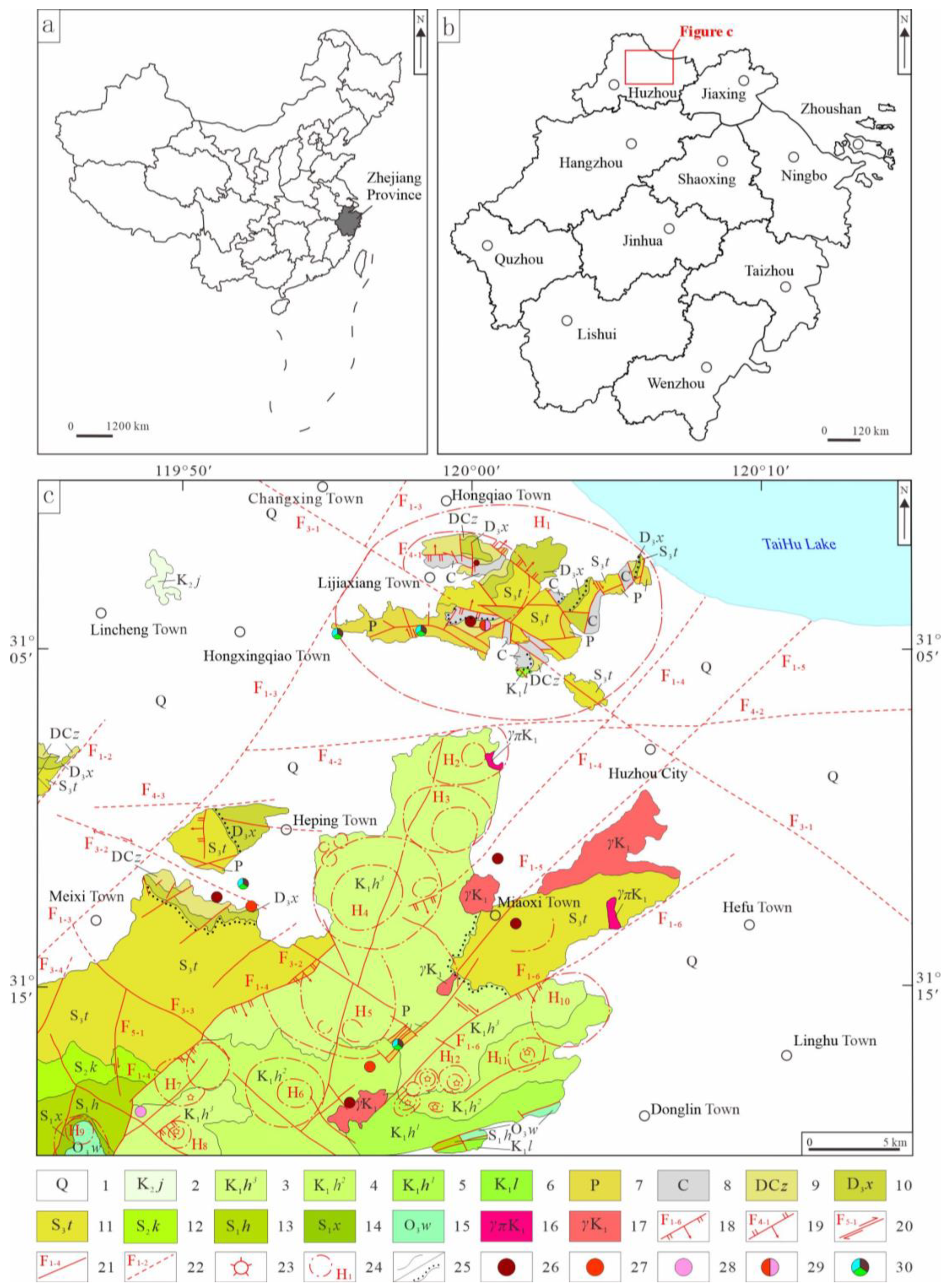
The study area (The Huzhou region) is situated in northern Zhejiang Province, China, along the southern bank of Lake Taihu. Spanning approximately 1767.77 km², the region extends from 119°14′00″ E–120°29′00″ E in longitude and from 30°22′00″ N–31°11′00″ N in latitude. The terrain generally slopes from southwest to northeast, with the western part consisting mainly of mountains and hills, while the eastern part is flat. The region receives abundant rainfall, resulting in lush vegetation. In terms of tectonic setting, the study area is located in the eastern part of the Yangtze Craton and forms part of the Lower Yangtze Metallogenic Belt, situated within the Changxing-Taihu compound fold belt. The regional geological and tectonic evolution is complex, having successively undergone multiple tectonic phases, including the Caledonian collisional aorogeny, the Indosinian intra-continental orogeny, the Yanshanian active continental margin development, and the Himalayan tectonic uplift. These processes have formed a rich array of geological structures, creating a favorable geological setting for mineralization.

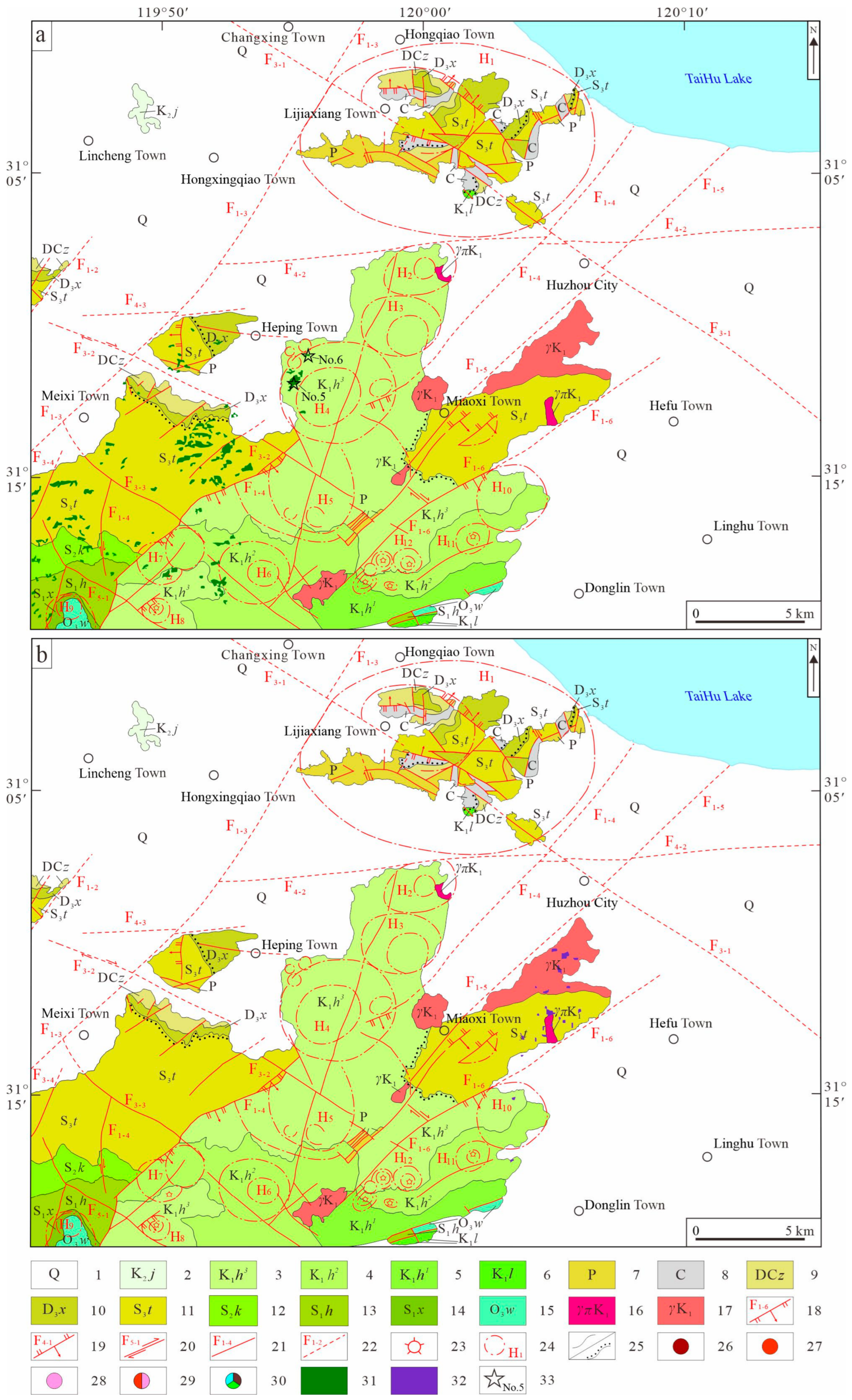
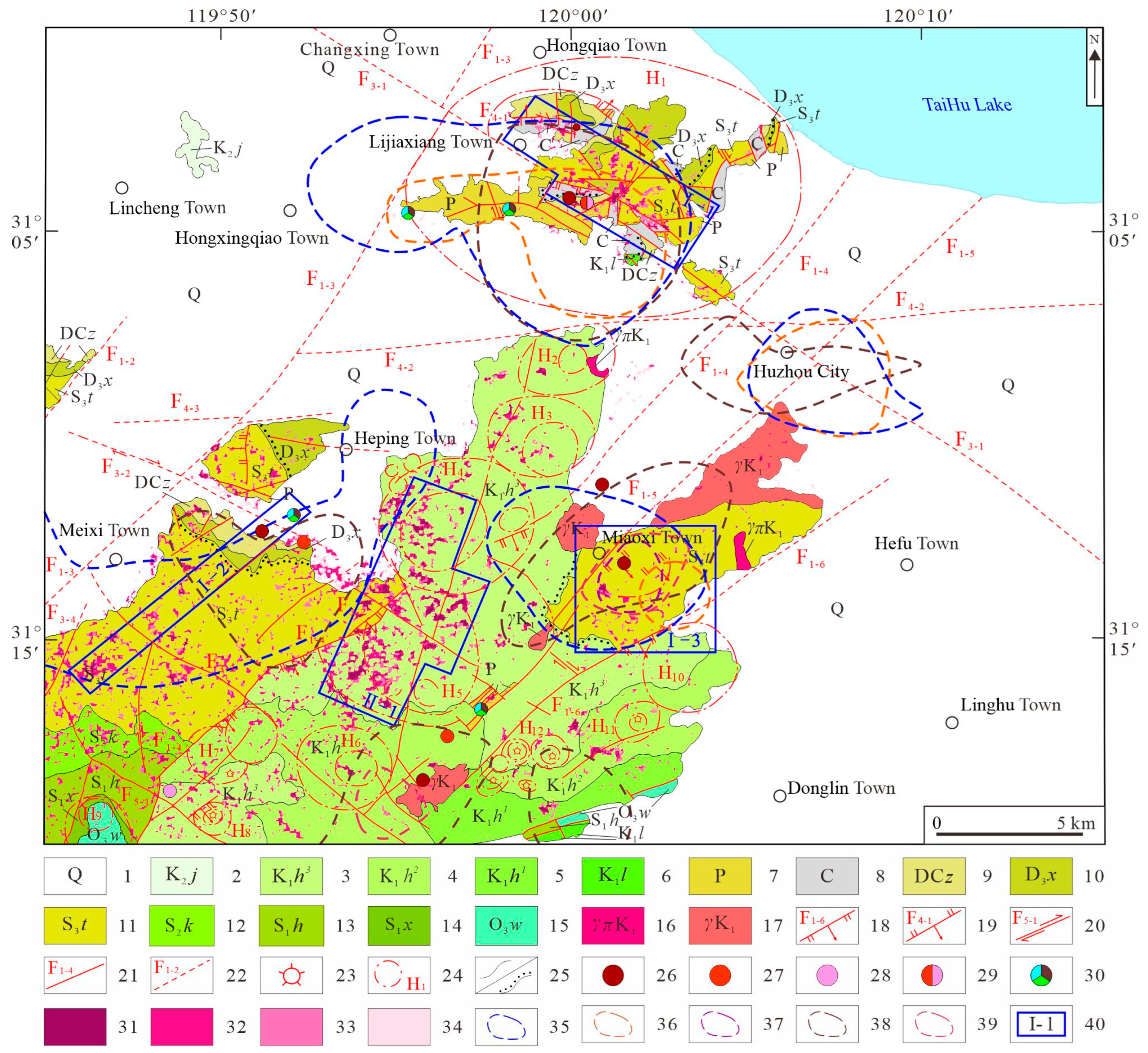
The strata exposed in the study area include the Ordovician, Silurian, Devonian, Carboniferous, Permian, Cretaceous, and Quaternary systems, with both sedimentary and volcanic rocks present (Figure 1). Among these, the Ordovician is represented solely by the Wenchang Formation (O₃w) of the Upper Ordovician Series, consisting of gray, thick-bedded, blocky feldspar-quartz sandstone and siltstone. The Silurian System is represented by the Xiaxiang Formation (S₁x) and Helixi Formation (S₁h) in the Lower Series, the Kangshan Formation (S₂k) in the Middle Series, and the Tangjiawu Formation (S₃t) in the Upper Series. The Xiaxiang Formation (S₁x) consists of bluish-gray, blocky, siltaceous mudstone; the Helixi Formation (S₁h) consists of interbedded bluish-gray siltstone and muddy siltstone; the Kangshan Formation (S₂k) consists of interbedded bluish-gray to gray-green siltstone and fine sandstone with well-developed bedding; and the Tangjiawu Formation (S₃t) consists mainly of light purplish-red and grayish-yellow fine-grained quartz sandstone interbedded with siltstone and mudstone. The Devonian System is represented solely by the Upper Devonian Xihu Formation (D₃x), consisting of grayish-white, medium-to-thick-bedded quartz sandstone, gravelly sandstone, siltstone, and mudstone. The Devonian–Carboniferous Zhuzangwu Formation (DCz) consists of clastic quartz sandstone and feldspathic clastic sandstone interbedded with silty mudstone. The Carboniferous System is represented by the Upper Series’ Laohudong Formation (C₂l) and Huanglong Formation (C₂h). Both of which have a relatively limited distribution; the lithology consists primarily of dolostone and limestone. The Permian strata are exposed only in a small area near Lijiaxiang, and the lithology consists mainly of limestone, siliceous rock, and siltstone. The Cretaceous System is represented by the Lower Cretaceous Laocun Formation (K₁l) and Huangjian Formation (K₁h), and the Upper Cretaceous Jinhua Formation (K₂j). The Laocun Formation (K₁l) consists of light gray glassy tuff and purplish-red conglomerate interbedded with siltstone; the Huangjian Formation (K₁h) is divided into three members, with lithologies consisting of rhyolitic clastic glassy welded tuff, andesitic clastic glassy welded tuff, and rhyolitic brecciated welded tuff, respectively; the Jinhua Formation (K₂j) consists of rhythmically interbedded purplish-red muddy siltstone and siltstone.

Plutonic exposures occupy a limited areal extent across the study region, comprising predominantly Early Cretaceous equigranular medium- to fine-grained granites and granodiorites. They are mainly concentrated in the area between Miaoxi Town and downtown Huzhou, with granodiorite and other intrusive bodies developed at depth.

The regional tectonic framework is primarily controlled by the northeast-trending Xuechuan–Huzhou Fault. This fault is a major regional fault in northwestern Zhejiang Province; it traverses the central part of the study area, with a general strike of 40–50°, a dip direction toward the southeast, a dip angle of 70–80°, a main width of 3–5 km, and an influence zone of approximately 15–20 km. It consists of a series of northeast-trending secondary faults. The fault is exposed within the study area, extending from Taipingqiao through Miaoxi Town to Huzhou City. The main fault zone is located in the Wushuwu area of Huzhou, manifesting as a strongly silicified alteration zone 300–500 m wide. Overall, the area is characterized primarily by a structurally fractured zone, a strongly silicified alteration zone, and cleavage and jointing. The Xuechuan–Huzhou Fault plays a significant role in controlling the distribution of Early Cretaceous volcanic rocks and intrusions within the study area. Volcanic rocks are primarily distributed within the fault zone; on its western boundary, they exhibit a fault contact with the Silurian strata, while on the eastern boundary, they are overlain by Quaternary deposits. Intrusions are mainly aligned along the strike of the main fault and exhibit a string-of-pearls distribution, reflecting the constraining effect of the fault on magmatic activity. In addition, NW-trending and nearly N-S-trending faults are also well-developed within the area. Multi-phase, multi-directional faulting often cuts through and modifies early-stage structures, collectively forming the complex tectonic system of the study area [67].

The regional geology is highly favorable for mineralization, and the area is rich in mineral resources. Currently, deposits of gold, silver, copper, iron, and uranium have been identified. The host-rock alteration, which is closely related to mineralization, is intense and exhibits a wide variety of types, including hematite and limonite mineralization, as well as montmorillonite alteration, sericite alteration, and chlorite alteration. These alteration minerals not only serve as important indicators for mineral exploration but also provide direct evidence for elucidating the nature of mineralizing fluids and process.

2.2. GF-5B Hyperspectral Data Used

The GF-5 satellite is a full-spectrum hyperspectral satellite designed for comprehensive observation of both the atmosphere and land surfaces. The GF-5B satellite is an operational satellite managed by the China Resource Satellite Application Center [55,68,69,70] and is China’s first comprehensive integrative observation satellite capable of hyperspectral, multispectral, and multi-angle observations.

The GF-5B satellite orbits at an altitude of 705 km and is equipped with the Environment Monitoring Instrument (EMI), the Greenhouse-gases Monitoring Instrument (GMI), the Directional Polarization Camera (DPC), the Atmospheric Infrared Ultraspectral Sensor (AIUS), the Advanced Hyperspectral Imager (AHSI), and the Infrared Multispectral Sensor (VIMS) [71]. The AHSI aboard GF-5B captures images across 330 spectral bands in the visible, near-infrared, and short-wave infrared (SWIR) regions. Specifically, 150 visible–near-infrared (VNIR) bands have a spectral resolution of 4.33 nm, and 180 short-wave infrared (SWIR) bands have a spectral resolution of 8.546 nm. All bands have a spatial resolution of 30 m and a swath width of 60 km (

Table 1. Main parameters of GF-5B AHSI hyperspectral data.

Spectral Band Category	Number of Bands	Spectral Range (nm)	Spectral Width (nm)	Spatial Resolution (m)	Swath Width (km)
VNIR	150	387–1024	4.330	30	60
SWIR	180	1009–2515	8.546

). This study utilizes GF-5B hyperspectral imagery acquired on 11 January 2023, as Level 1 data. The dataset includes GeoTIFF data files, XML metadata files, RPC parameter files, thumbnail files, coverage vector files, observation geometry files, and calibration parameter files.

3. Methods

3.1. Process for Extracting Alteration Minerals

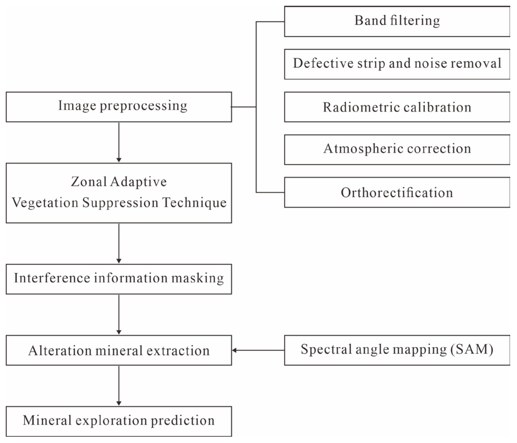
This investigation employs GF-5B hyperspectral satellite (China) imagery acquired over Huzhou City, Zhejiang Province, China, as its data source to conduct research on the extraction of alteration minerals and mineral exploration prediction. The technical methodology comprises a sequence of procedures: image preprocessing, vegetation suppression, masking of interference information, alteration mineral extraction, and mineral exploration prediction (Figure 2). (1) Preprocessing of the raw hyperspectral imagery includes band filtering, defective strip repair and noise removal, radiometric calibration, atmospheric correction, and orthorectification, to improve image quality and spectral accuracy. Specifically, band filtering is used to remove bands affected by water vapor absorption, bands with low signal-to-noise ratios, and bands with overlapping detector ranges. Mean filtering is employed to repair damaged bands and is combined with global debanding to remove striped noise. Radiometric calibration is used to convert pixel grayscale values to radiance values. Atmospheric correction is performed using the FLAASH model within ENVI 5.3 software to eliminate atmospheric interference caused by factors such as atmospheric scattering, thereby obtaining true surface reflectance. Finally, orthorectification is performed to eliminate geometric distortions caused by terrain, camera geometry, and sensor-specific errors. (2) Building on the image preprocessing, a zone-based adaptive vegetation suppression technique is employed to reduce the interference of vegetation spectra on the extraction of alteration minerals. (3) Masking is applied to water bodies, areas with high vegetation cover, and Quaternary-covered areas to minimize the impact of interfering features on alteration mineral extraction, yielding hyperspectral image data suitable for alteration mineral interpretation. (4) Typical spectra of alteration minerals from the U.S. Geological Survey (USGS) standard spectral library are selected as reference endmembers. Using the spectral angle mapping (SAM) method, the similarity between the image spectra and the reference endmember spectra is calculated on a pixel-by-pixel basis to identify and extract Fe-bearing alteration minerals, Al-OH type alteration minerals, and Mg-OH type alteration minerals. (5) By integrating information on fault structures, stratigraphic sequences, known mineral deposits (locations), elemental anomalies, and the distribution of alteration minerals derived from remote sensing interpretation, prospective exploration areas are delineated, thereby providing a scientific basis for regional mineral resource exploration.

3.2. Zonal Adaptive Vegetation Suppression Technique

As the primary land cover type, dense vegetation canopies often obscure the underlying bedrock, resulting in mixed pixels containing both vegetation and rock signals. Vegetation exhibits strong spectral responses in the visible range (with chlorophyll strongly absorbing near 450 nm and 670 nm), the near-infrared range (characterized by strong reflectance between 760 and 1300 nm), and the SWIR range (with pronounced absorption due to water content). These features overlap significantly in wavelength with the diagnostic absorption wavelength of alteration minerals, such as Fe-bearing alteration minerals (500–1100 nm) and hydroxyl-bearing minerals (near 2200 nm), leading to the masking or distortion of target information. Without effective vegetation suppression processing, alteration minerals are difficult to extract effectively; even when they are detected, they typically appear weak, scattered, and discontinuous, making it difficult to meet the practical accuracy requirements of geological prospecting.

To mitigate vegetation interference in hyperspectral imagery and accentuate the spectral characteristics of subsurface lithological features, this study proposes a Zonal Adaptive Vegetation Suppression Technique (ZAVST). The core concept is to use the Normalized Difference Vegetation Index (NDVI) as the independent variable and construct statistical models of the relationship between land cover reflectance and NDVI on a band-by-band basis. Polynomial curve fitting is performed using the least squares method, and piecewise smoothing is applied to the curves to reduce the spectral contribution of vegetation, enhance the spectral characteristics of target objects such as rocks and soil, and improve the detectability of altered mineral information. The operational workflow comprises the following sequential stages.

(1)

Calculate the Normalized Difference Vegetation Index (NDVI). This index is calculated using the near-infrared and red spectral bands. This index is highly sensitive to the growth status of green vegetation, making it effective for monitoring vegetation growth and estimating vegetation cover. To facilitate land cover classification and segmented interval indexing, the original floating-point range of NDVI [−1, 1] is linearly stretched to the integer range [0, 255]. However, when actually used in the calculation of the vegetation contribution separation formula (1), the original floating-point NDVI values are still employed.

(2)

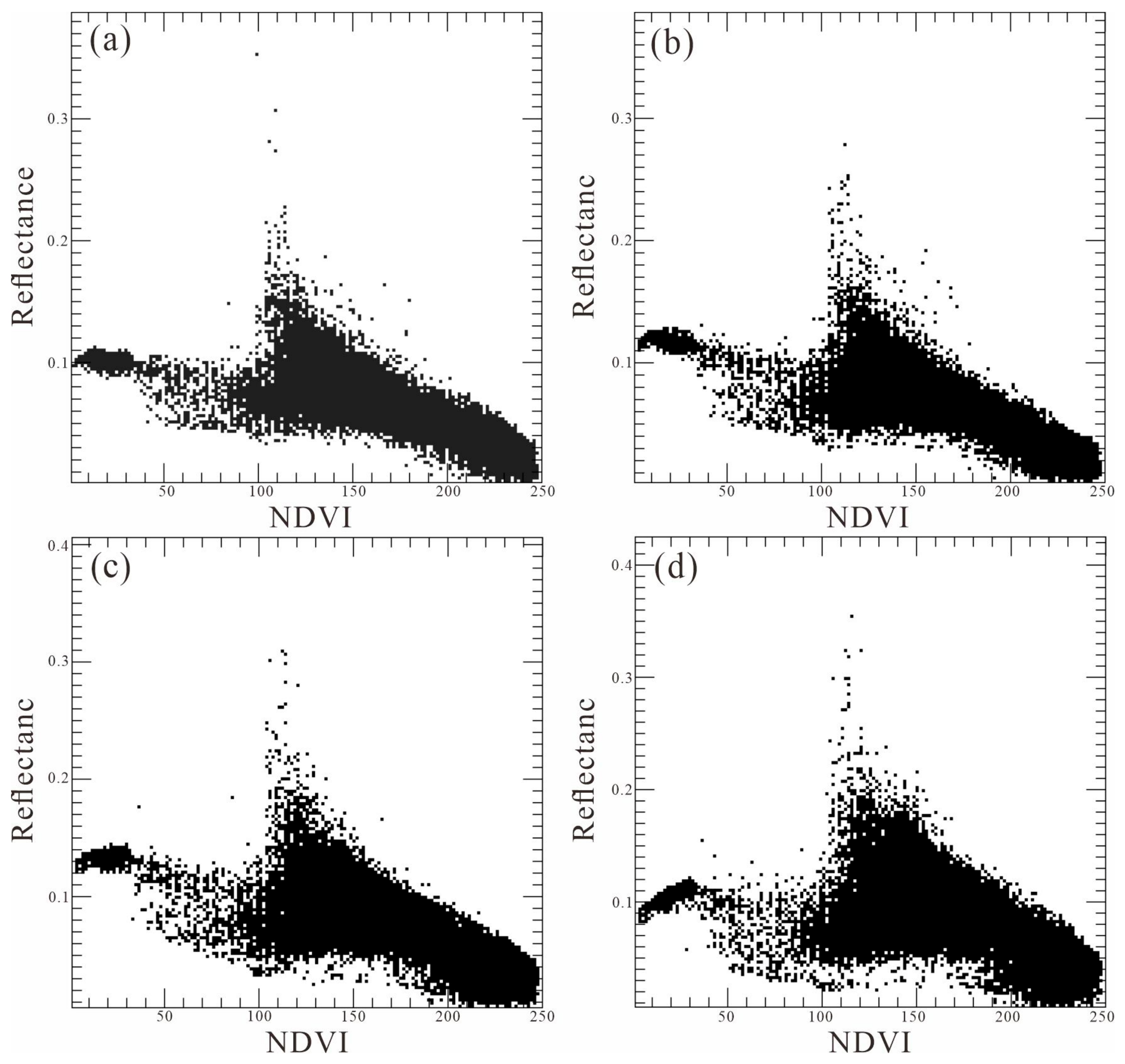
Analyze the relationship between reflectance in each band and NDVI. Perform scatter plot analysis on each band of the preprocessed hyperspectral imagery against the NDVI imagery. For each band, statistically analyze the distribution relationship between the reflectance of each pixel and its corresponding NDVI value, and generate scatter plots. To eliminate the interference of outliers in the imagery on the overall trend analysis, this study employs a mean-based fitting method with percentile filtering to perform curve fitting on the multivariate scatter data. First, the 25th and 75th percentiles of the reflectance values are calculated to define the valid data range. Only the image reflectance data falling between the 25th and 75th percentiles are retained, thereby excluding outliers and extreme discrete points outside this range. Next, for each NDVI value, the arithmetic mean of its corresponding reflectance values is calculated. The mean points at each NDVI location are then connected sequentially to form a mean curve, which visually reflects the overall trend of the main data set. This fitted curve reveals the general trend of reflectance variation with vegetation cover, providing a basis for subsequent segmented smoothing processing.

(3)

Classify land cover based on NDVI. Based on the mean and standard deviation of NDVI, and in conjunction with the distribution patterns observed in scatter plots and fitted curves, the image is divided into regions corresponding to different land cover types: areas where NDVI > (mean + 0.5 × standard deviation) are classified as vegetation; areas where NDVI < 0 are classified as water bodies, clouds, and shadows; areas where 0 < NDVI < (mean + 0.5 × standard deviation) are classified as Quaternary deposits and other land cover types. In southern vegetation-covered regions, where land cover types are complex and diverse and spectral values are highly dispersed, land cover classification should emphasis overall consistency and avoid excessive subdivision.

(4)

Calculate the segmented smoothed values. To reduce random errors in the fitted curves, this study further smooths the fitted curves for each band using a method that combines median filtering with local weighted averaging. First, median filtering is applied to perform preliminary smoothing of the fitted curves. As a nonlinear smoothing technique, median filtering replaces the value at each point on the curve with the median of all values in that point’s neighborhood. This step effectively suppresses isolated noise points while preserving the edge features of the curve, thereby avoiding the blurring of transition zones between different land cover types caused by excessive smoothing. Building on this, segmented smoothing is further performed using the local weighted averaging method. This method divides the curve into several segments based on the distribution characteristics of land cover types. Within each segment, the values at each point on the curve are calculated using a weighted average based on the values of several neighboring points, with closer points assigned higher weights, thereby achieving refined smoothing within a local area. After these two processing steps, we obtain smoothed curves showing how reflectance varies with NDVI values for each band. Fluctuations within each NDVI interval have been effectively suppressed, and random noise caused by changes in vegetation cover has been largely eliminated. Finally, for each NDVI interval, we calculate the average reflectance of all corresponding points on the smoothed curve to obtain the segmented average value for that band within that interval (Ptarget).

(5)

Smooth segmented curves and separate vegetation contributions. The core of this step lies in quantitatively separating and removing the spectral contribution of vegetation to achieve vegetation suppression, thereby highlighting the spectral characteristics of target objects such as rocks and soil. Specifically, for each pixel, based on the bin in which its NDVI value falls, the corresponding flat-field value for that band is selected. The original reflectance value is then adjusted as a ratio to separate the spectral contribution of vegetation, yielding a new pixel value. Equation (1) for separating the vegetation contribution is as follows:

$$P_{\mathrm{new}}=P_0{\displaystyle \frac{P_{\mathit{target}}}{\mathit{NDVI}}}$$

(1)

where $P_{\mathit{new}}$ represents the new image reflectance value, $P_0$ represents the original image reflectance value, NDVI represents the Normalized Difference Vegetation Index, and P_target represents the flat-field value.

3.3. SAM Method

The SAM method for identifying altered minerals is based on the overall similarity of spectral curves. It treats the spectral data of each pixel in a hyperspectral image as a vector in a high-dimensional space and measures the degree of spectral similarity by calculating the angle between the spectral curve of an image pixel and the spectral curve of a standard mineral. The smaller the angle, the more similar the two spectra are, and the greater the likelihood that the corresponding pixels represent the same type of geological feature. Therefore, the category of an unknown pixel can be determined based on the magnitude of the spectral angle, thereby enabling the qualitative identification of altered minerals. The mathematical expression of SAM is based on the law of cosines, quantifying the degree of similarity by calculating the cosine of the angle between the two spectral vectors. Equation (2) is as follows:

$$\mathit{SAM}\left(x,y\right)=\mathit{arccos}{\displaystyle \frac{{\displaystyle {\sum }_{i=1}^n}{x}_i{y}_i}{\sqrt{{\displaystyle {\sum }_{i=1}^n}{x}_i^2}\sqrt{{\displaystyle {\sum }_{i=1}^n}{y}_i^2}}}$$

(2)

where $x$ represents the spectral vector of a hyperspectral image pixel, $y$ represents the standard mineral spectral vector, $n$ represents the number of bands used in the calculation.

Compared to traditional band ratio methods and principal component analysis, SAM places greater emphasis on matching the overall shape of spectral curves. It can effectively reduce interference caused by factors such as terrain shadows and variations in illumination, making it more suitable for identifying altered minerals with diagnostic spectral absorption troughs. Although SAM is sensitive to the overall spectral shape, the spectral data of individual pixels in the acquired images are often affected by factors such as sensor noise and residual atmospheric correction, leading to spectral distortion or local disturbances that can easily cause deviations in SAM calculation results. Therefore, in practical applications, SAM is often combined with processing techniques such as envelope removal and Savitzky–Golay filtering to improve the accuracy of altered mineral extraction.

4. Image Preprocessing

4.1. Basic Preprocessing

The basic preprocessing of GF-5B hyperspectral data mainly includes band filtering, defective strip and noise processing, radiometric calibration, atmospheric correction, and orthorectification. The GF-5B hyperspectral imager acquires data across 330 spectral bands, including 150 visible–near-infrared (VNIR) bands and 180 short-wave infrared (SWIR) bands. Spectral regions corresponding to strong water vapor absorption features (1356–1447 nm, 1800–1982 nm, and 2375–2395 nm) require exclusion during mineralogical analysis due to significant atmospheric attenuation effects. Following systematic analysis of GF-5B hyperspectral data, 52 spectral channels were removed based on comprehensive quality assessment criteria categorized into three groups: atmospheric absorption features, low SNR bands, and detector overlap artifacts. This preprocessing workflow resulted in the retention of 278 scientifically valid bands for subsequent alteration mineral mapping (

Table 2. A list of excluded bands for GF-5B hyperspectral data.

Band Number	Wavelength Position (nm)	Reason for Removal	Spectral Band Category	Number of Bands Removed
band 1–3	387–395	Low SNR	VNIR	4
band 150	1024	Low SNR
band 151–153	1009–1025	Overlap with VNIR data	SWIR	48
band192	1354	Low SNR
band 193–200	1362–1421	Water vapor absorption band
band 201–206	1429–1471	Low SNR
band 245–262	1800–1943	Water vapor absorption band
band 263–265	1951–1968	Low SNR
band 269–271	2002–2018	Low SNR
band 325–330	2473–2515	Low SNR

).

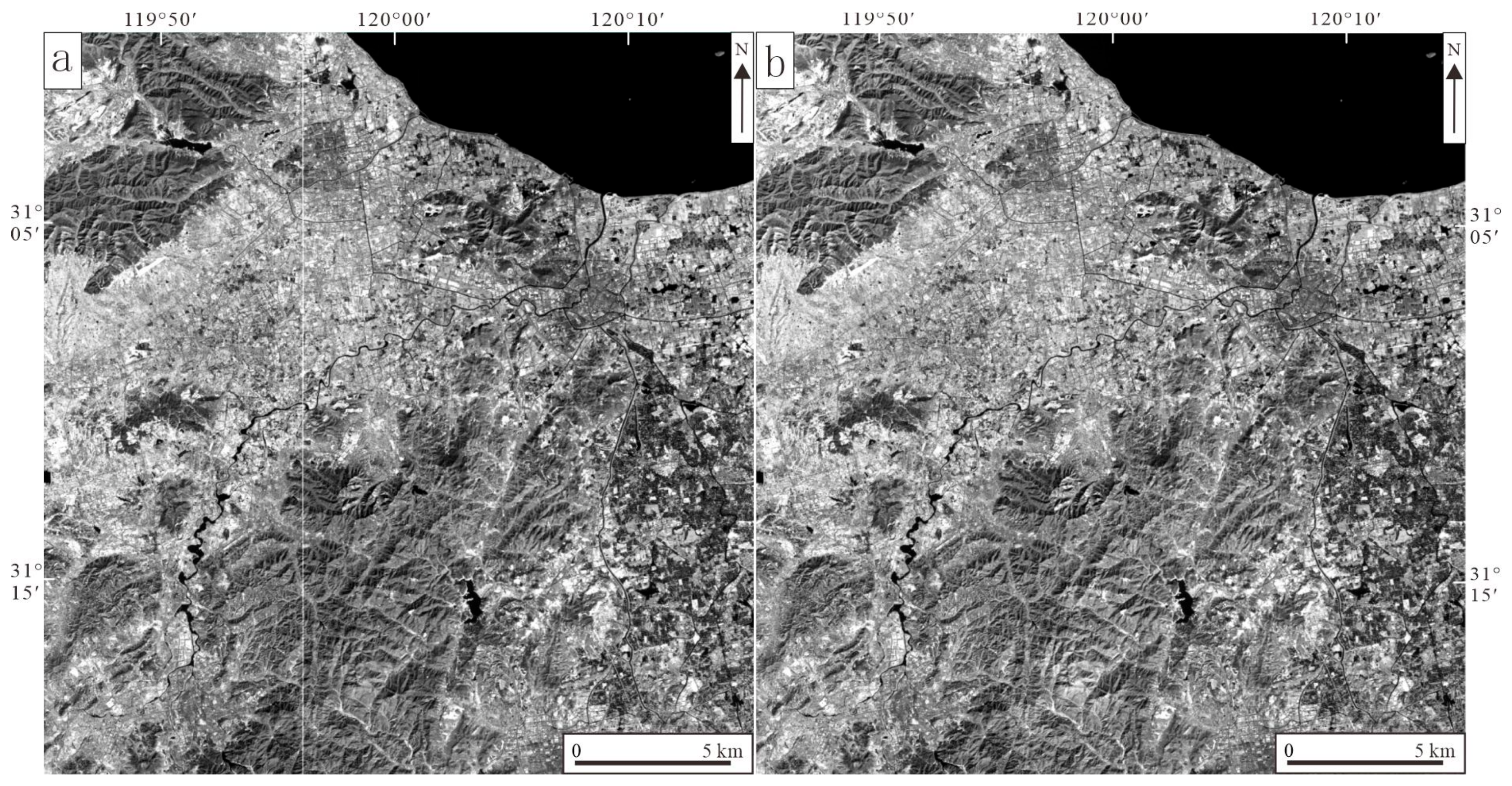
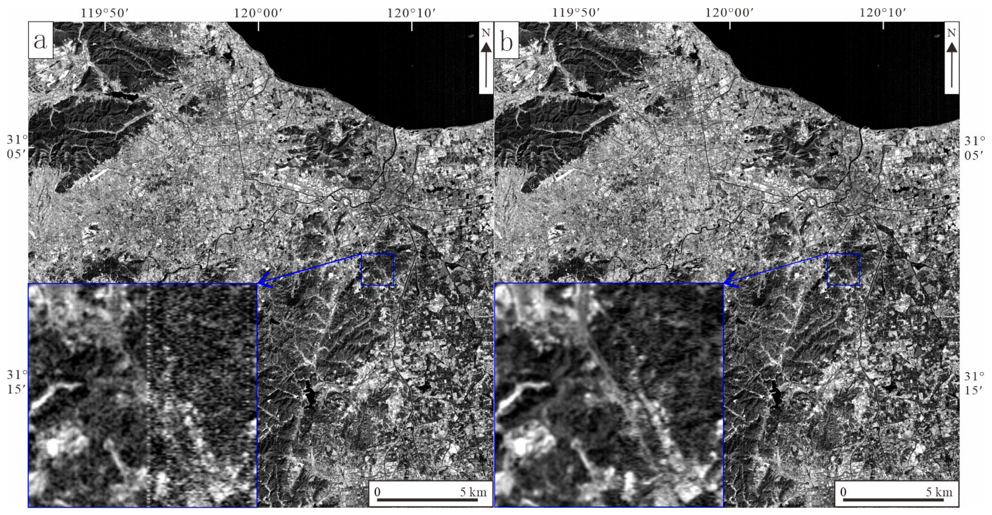
After band filtering and spectral profile inspection, it was observed that in certain bands, the pixel values of some rows or columns are abnormally high or low, appearing as sharp peaks or troughs in the spectral profile, which correspond to bright or dark regions in the image, commonly referred to as “bad lines.” A band-by-band examination revealed that the bad lines are mainly distributed in the SWIR bands, and some of them occur at the same positions across different bands, showing a regular distribution pattern. This study employs a mean filtering method for restoration, using the average pixel values of adjacent columns or rows on both sides of the bad line to replace the anomalous pixel values at the bad line positions (Figure 3). The proposed methodology successfully corrected 287 striping artifacts across affected spectral bands.

The GF-5B hyperspectral imager utilizes a pushbroom scanning mechanism where inherent sensitivity discrepancies among detector elements introduce systematic striping artifacts into acquired radiance data. These artifacts visually present as periodic intensity deviations along the scan direction, manifesting as alternating bright/dark bands that degrade radiometric consistency and spatial homogeneity. This study implements the global debanding method [19] to remove striping noise using Python 3.9 programming. Equation (3) for this method is as follows.

$${X^{\prime }}_{\mathit{ijk}}={\alpha }_k{X}_{\mathit{ijk}}{+\beta }_k$$

$${\alpha }_k=\overline{s_k}/s_{\mathit{ik}}$$

$${\beta }_k=\overline{m_k}-{\alpha }_{\mathit{ik}}{m}_{\mathit{ik}}$$

(3)

where ${X^{\prime }}_{\mathit{ijk}}$ represents the grayscale value at row i and column j in the kth band of the corrected image; $X_{\mathit{ijk}}$ represents the grayscale value at row i and column j in the kth band of the original image; ${\alpha }_k$ represents the gain value of the sensor’s kth band; ${\beta }_k$ represents the offset value of the sensor’s kth band; $\overline{s_k}$ represents the standard deviation of the kth band in the reference image; $s_{\mathit{ik}}$ represents the standard deviation of column i in the kth band of the image to be processed; $\overline{m_k}$ represents the mean value of the kth band in the reference image; $m_{\mathit{ik}}$ represents the mean value of column i in the kth band of the image to be processed.

Using the methods described above, this study processed striped noise across 18 spectral bands. A comparison of the images before and after processing shows a significant improvement in image quality (Figure 4).

Atmospheric correction is performed by removing atmospheric attenuation effects (such as scattering and absorption), thereby obtaining more accurate surface reflectance information. This study uses the Radiometric Calibration tool in ENVI 5.3 to perform radiometric calibration on remote sensing images and employs the FLAASH (Fast Line-of-sight Atmospheric Analysis Spectral Hypercube) model to carry out atmospheric correction on the imagery of the study area. Equation (4) is as follows:

$$L_{\lambda }=\mathit{Gain}\times \mathit{DN}+\mathit{Offset}$$

(4)

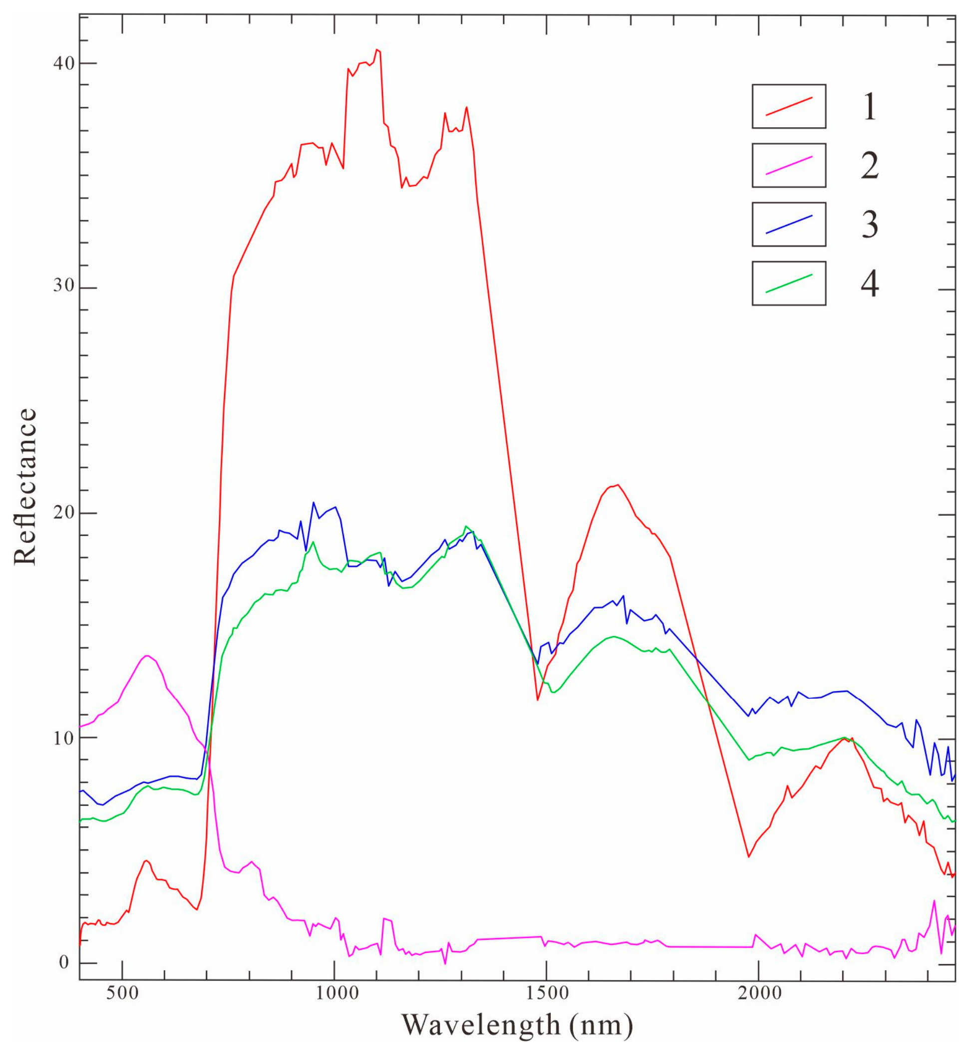
where $L_{\lambda }$ represents radiant luminance; DN represents the image grayscale value; Gain represents the gain value; and Offset represents the offset value.The parameter information for atmospheric correction is shown in

Table 3. A list of atmospheric correction parameters for GF-5B hyperspectral data.

Atmospheric Correction Parameters Details	Atmospheric Correction Parameter Settings
Image center coordinates	30.8248° E; 119.9128° N
Sensor altitude	705 km
Mean ground elevation	0.069 km
Image acquisition time	2023-1-11; UTC 2:52:56
Atmospheric model	Mid-Latitude Summer (MLS)
Water vapor retrieval band	1135 nm
Aerosol model	Rural
Initial visibility	30 km
Spectral smoothing	YES
Block processing	NO

. After atmospheric correction, the reflectance data were amplified by a factor of 10,000; therefore, it required further scaling through band-specific calculations to obtain hyperspectral reflectance data with a numerical range of 0.0–1.0 (Figure 5).

After completing radiometric calibration, atmospheric correction, and other processing steps, metadata information is retained in the imagery, and RPC parameters are automatically embedded in the processed results. Therefore, RPC orthorectification can be further performed based on the atmospherically corrected imagery. This study selected Landsat-8 OLI data (imaged on 20 January 2023) with a timing close to that of the GF-5B imagery as the reference image for orthorectification. ASTER GDEM was used as the elevation calibration data, and the RPC module in ENVI 5.3 was employed to perform orthorectification on the GF-5B imagery. After orthorectification, the geographic positioning accuracy of the imagery was significantly improved, and anomalies in pixel values caused by terrain undulations were also mitigated. Finally, the orthorectified imagery was cropped according to the study area boundaries to obtain the preprocessed target imagery of the study area.

4.2. Zonal Adaptive Vegetation Suppression Technique Processing

The vegetation suppression processing in the study area includes the following key steps:

NDVI Calculation and Stretching. Using orthorectified imagery as the data source, the NDVI was calculated using the red band (B63) and the near-infrared band (B112). Statistical analysis revealed that the mean of the NDVI imagery was 0.36, with a standard deviation of 0.30. To facilitate subsequent calculations, the floating-point range of NDVI [−1, 1] was linearly stretched to the integer range [0, 255]. The mean of the stretched NDVI image became 169.62, with a standard deviation of 48.70. Based on this, scatter plots were generated showing the relationship between the reflectance of each band and NDVI (Figure 6).

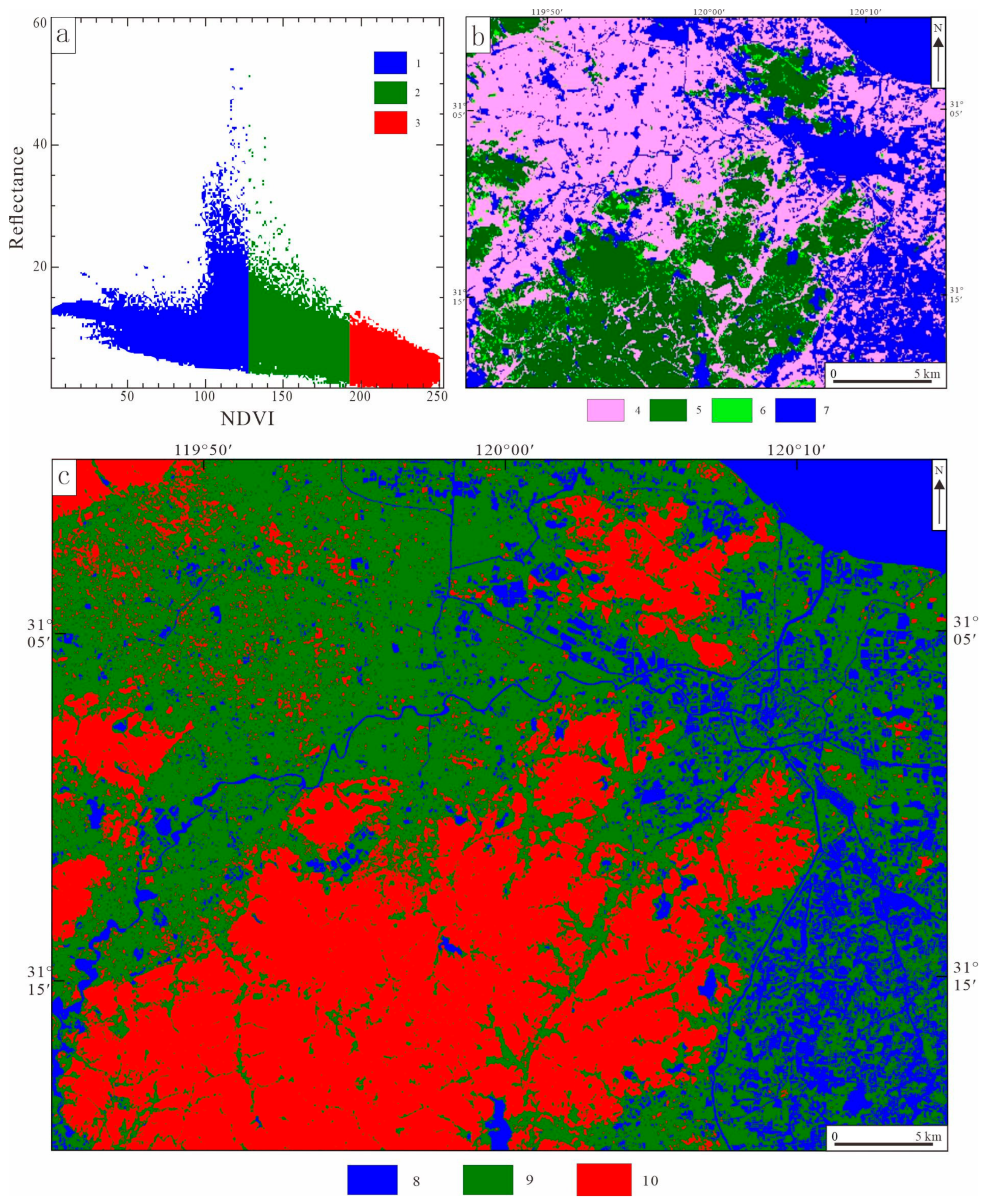
Land cover classification and region of interest (ROI) assignment. Land cover was classified based on NDVI values, colored, and plotted as an ROI scatter plot (Figure 7a). The classification criteria were as follows: areas with NDVI > (mean + 0.5 × standard deviation) were classified as vegetation; areas with NDVI < 0 were classified as water, clouds, and shadow; areas where 0 < NDVI < (mean + 0.5 × standard deviation) were classified as Quaternary and other land cover zones. The corresponding integer NDVI ranges are vegetation zones [193, 255], water bodies and cloud/shadow zones [0, 128], and Quaternary and other zones [128, 193]. Based on this, an image land cover classification map was generated (Figure 7c). Comparison with the land cover classification map of the study area (Figure 7b) reveals that the map classification is effective and accurate.

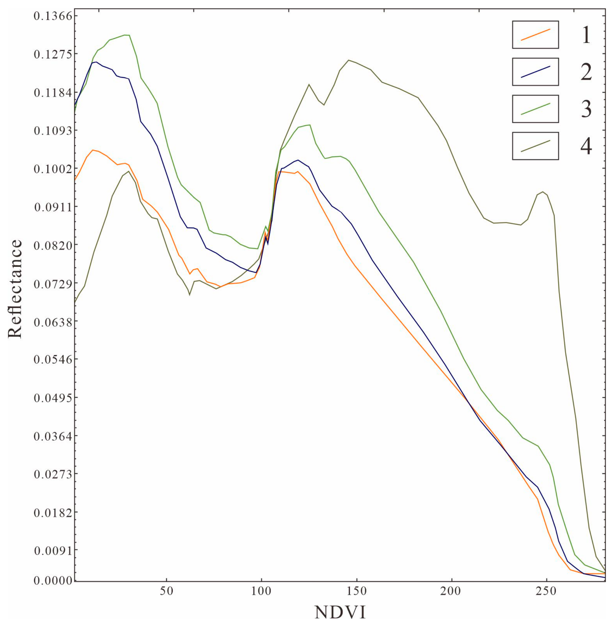
Statistical modeling and smoothing. For each band, curve fitting was performed on the multivalued scatter data using a mean-based fitting method with percentile-based filtering, with NDVI as the independent variable and band reflectance as the dependent variable. First, outliers and extreme outliers were removed, retaining only the core observation data located between the 25% and 75% percentiles. Based on this, statistical relationships between the reflectance of each band and NDVI were established. Subsequently, median filtering and locally weighted averaging smoothing were applied to the fitted curves within each band (Figure 8) to obtain the smoothed target values for each band (

Table 4. Segmented smoothed values of representative bands.

Bands	Segmented Smoothing Values Corresponding to NDVI
	[0, 128)	[128, 193)	[193, 255)
B4	0.08733	0.06146	0.03057
B27	0.09706	0.06598	0.03166
B48	0.10428	0.07887	0.04030
B74	0.09134	0.11625	0.08956

).

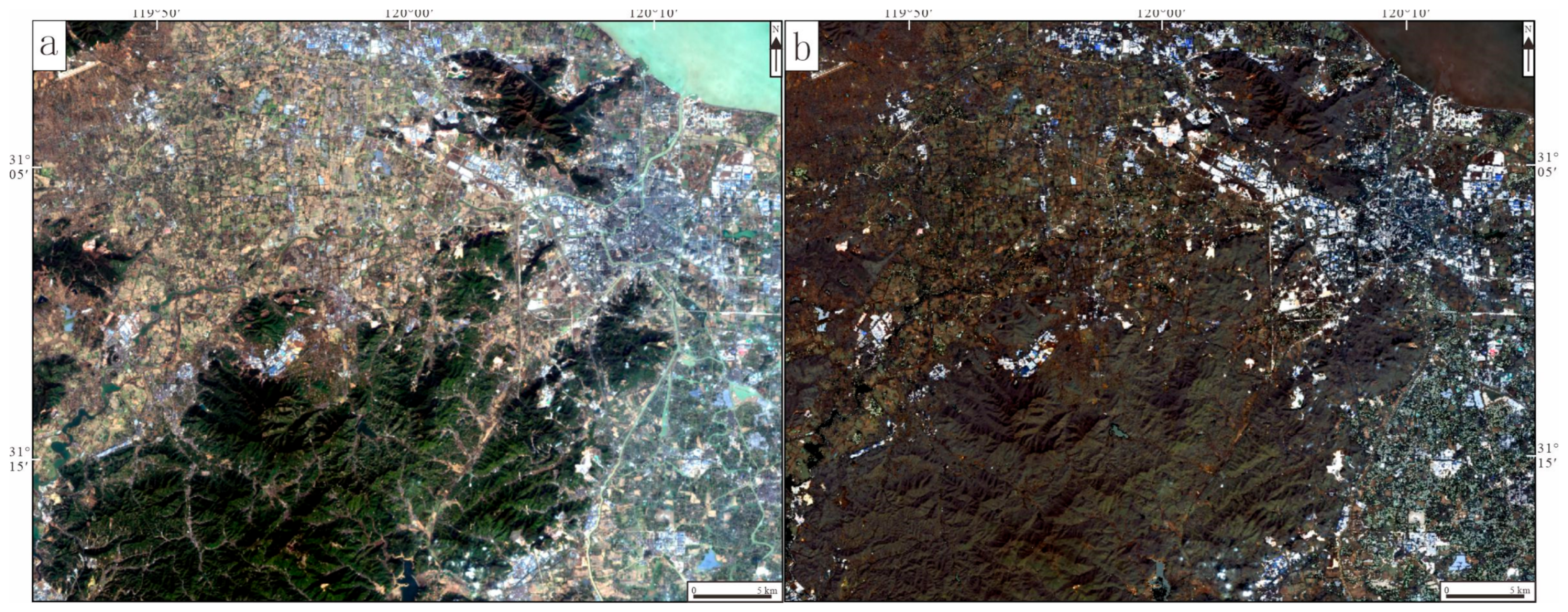
The segmented-smoothed values were substituted into Equation (1) to separate the spectral contribution of vegetation, and vegetation information was suppressed using Python programming (Figure 9).

The above processing workflow is implemented using Python. The core code is as follows:

def calculate_ndvi(red_band, nir_band):

•    ndvi = (nir_band − red_band) / (nir_band + red_band + 1e-10)
•    return ndvi

 

• def vegetation_suppression(img, red_index, nir_index):
•     red_band = img[red_index]
•     nir_band = img[nir_index]
•     ndvi = calculate_ndvi(red_band, nir_band)

 

•     num_segments = 10
•     segments = np.linspace(ndvi.min(), ndvi.max(), num_segments + 1)
•     suppressed_img = np.zeros_like(img)

 

•     for i in range(len(segments) − 1):
•         mask = (ndvi >= segments[i]) & (ndvi < segments[i + 1])
•         if np.any(mask):
•             for b in range(img.shape[0]):
•                 segment_values = img[b][mask]
•                 if len(segment_values) > 0:
•                     mean_val = np.mean(segment_values)
•                     suppressed_img[b][mask] = img[b][mask] − mean_val + np.mean(img[b])
•         else:
•             suppressed_img[:, mask] = img[:, mask]

return suppressed_img

In the images processed with vegetation suppression, the mean NDVI value in the study area decreased from 0.36 before processing to 0.29, a reduction of approximately 19.4%, indicating that the spectral contribution of vegetation was effectively separated; the standard deviation increased from 0.30 to 0.40, an increase of approximately 33.3%, indicating that the spectral differences among different land cover types were enhanced and the information dispersion was increased. From a quantitative perspective, these changes validate the effectiveness of the zone-based adaptive vegetation suppression technique proposed in this study in mitigating vegetation interference and highlighting the spectral characteristics of geological targets, thereby laying a solid data foundation for subsequent high-precision identification of altered minerals using SAM.

4.3. Interference Information Masking

In hyperspectral remote sensing, vegetated areas, aquatic systems, Quaternary sedimentary formations, and analogous surface features frequently demonstrate spectral signatures resembling hydrothermally altered minerals within characteristic absorption ranges. This can easily lead to confusion with genuine altered mineral information, resulting in “false anomalies” that hinder the effective extraction of altered mineral data. To mitigate the impact of these interferences, masking areas with high vegetation cover, water bodies, and Quaternary sediment deposits helps improve the signal-to-noise ratio and recognition accuracy of alteration mineral information. Based on the actual conditions of the study area, the primary interfering features—including vegetation, water bodies, and Quaternary sediments—were identified.

(6)

Vegetation and Quaternary sediment masking

To reduce interference from vegetation, areas with high vegetation cover were further masked after applying vegetation suppression to the imagery. Vegetation information was extracted using NDVI, calculated using Equation (5):

$$\mathit{NDVI}={\displaystyle \frac{\mathit{NIR}(\mathit{Band}112)-\mathit{RED}(\mathit{Band}63)}{\mathit{NIR}(\mathit{Band}112)+\mathit{RED}(\mathit{Band}63)}}$$

(5)

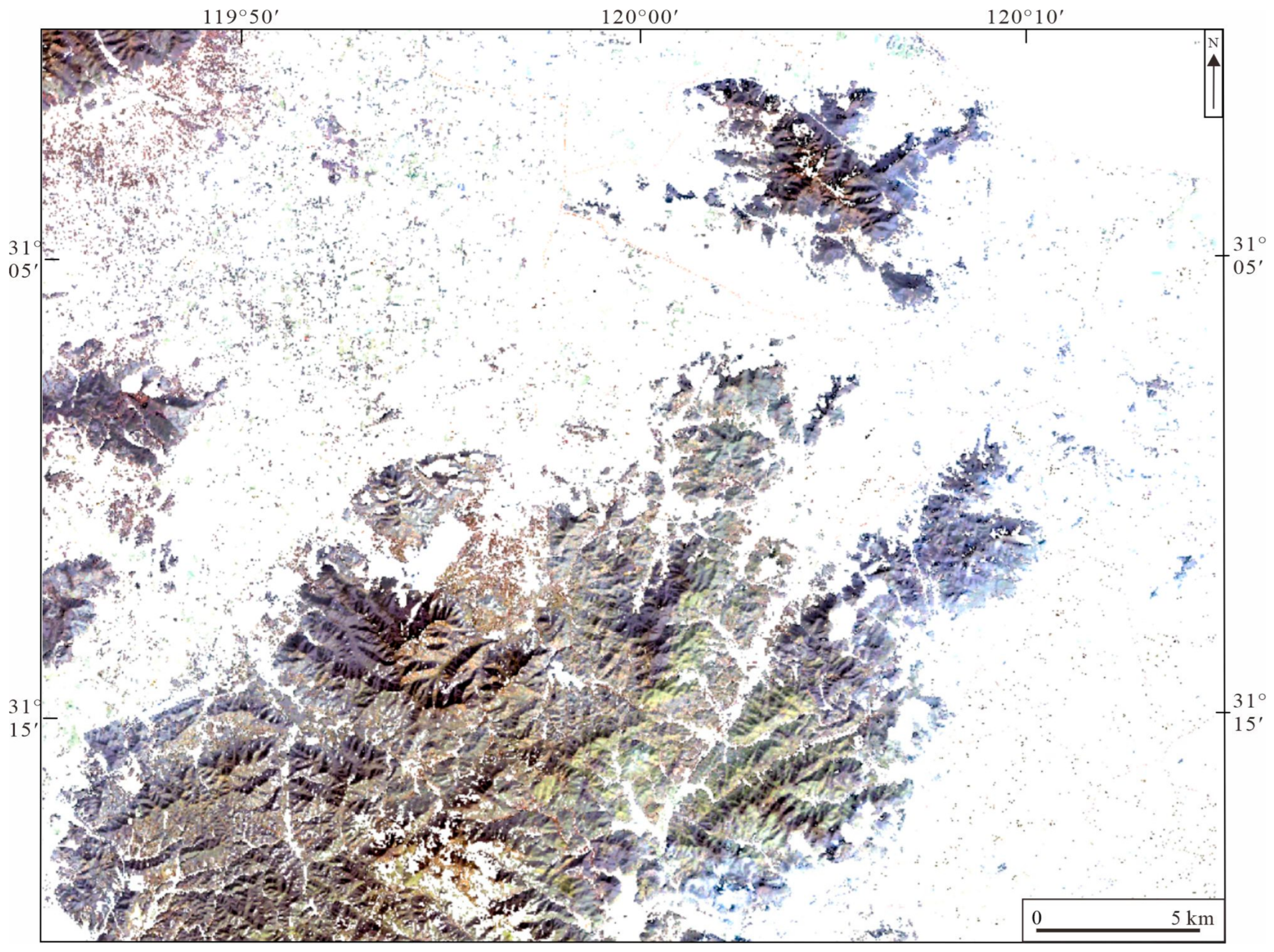
Based on the calculation results, the mean of the NDVI imagery was 0.36, and the standard deviation was 0.30. Areas with NDVI values greater than mean + 1.5 × standard deviation were classified as high vegetation cover areas and masked. Additionally, visual interpretation revealed that areas with NDVI values greater than 0 but less than mean + 0.5 × standard deviation largely corresponded to the distribution range of Quaternary deposits; therefore, this range was used as the masking range for Quaternary deposits and excluded from the analysis.

(7)

Water bodies masking

Water body information was extracted using the Modified Normalized Difference Water Index (MNDWI), calculated using Equation (6):

$$\mathit{MNDWI}={\displaystyle \frac{\mathit{GREEN}(\mathit{Band}41)-\mathit{SWIR}(\mathit{Band}112)}{\mathit{GREEN}(\mathit{Band}41)+\mathit{SWIR}(\mathit{Band}112)}}$$

(6)

Based on the calculation results, the mean value of the MNDWI image was −0.35, and the standard deviation was 0.29. Since non-water areas accounted for a large proportion of the image, areas with MNDWI values greater than the mean + 1.8 × the standard deviation were classified as water bodies; that is, masking was applied to areas where MNDWI > 0.19. The masked images showing dense vegetation, Quaternary deposits, and water bodies are shown in Figure 10.

5. Results

5.1. Extraction of Fe-Bearing Alteration Minerals

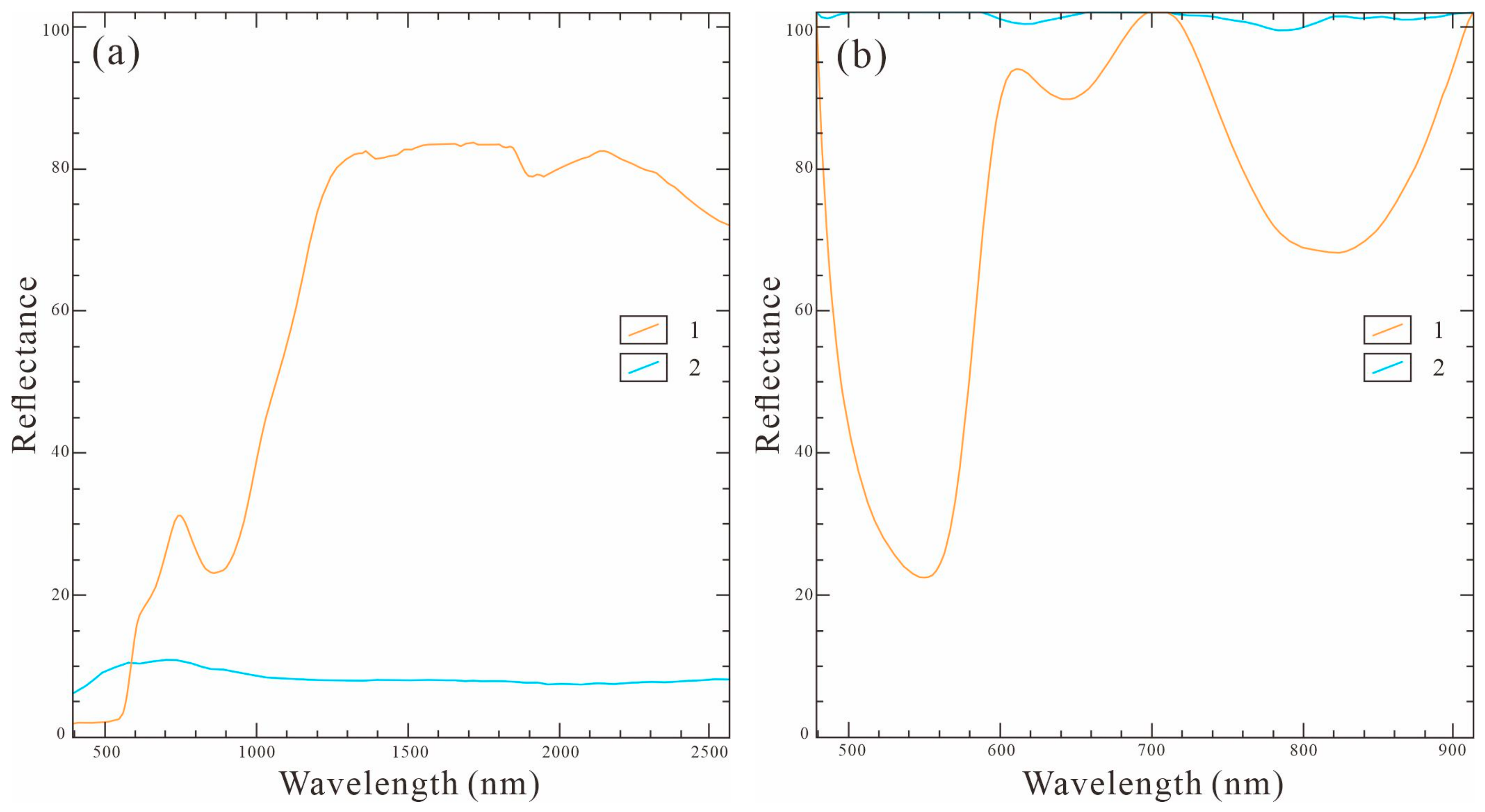
Diagnostic absorption features characteristic of alteration minerals at specific wavelengths provide the physical foundation for their identification through hyperspectral remote sensing techniques. According to spectral curve analyses, reflectance characteristics between 400 and 1300 nm are predominantly governed by electronic transitions involving Fe²⁺/Fe³⁺ ions within mineral crystal lattices. Based on the major alteration mineral types and their spectral characteristics in the study area, hematite and pyrite were selected from the U.S. Geological Survey (USGS) standard spectral library as target mineral spectra (Figure 11a).

Diagnostic absorption features of Fe-bearing minerals predominantly occur within the 400–1300 nm range. For GF-5B hyperspectral data processing, we selected the 451–998 nm range as the optimal resampling range for alteration mineral detection through empirical validation. Raw spectral measurements contain high-frequency noise artifacts from sensor calibration residuals, which deviate from true surface reflectance signatures of geological targets. Spectral smoothing was implemented using the Savitzky–Golay filter (window size = 11, polynomial order = 3) to suppress high-frequency noise while preserving diagnostic absorption features. Based on this, the smoothed spectral curves were further processed to remove the spectral envelope, thereby highlighting the absorption trough patterns of different altered minerals (Figure 11b) and improving the accuracy of mineral identification in subsequent SAM processing.

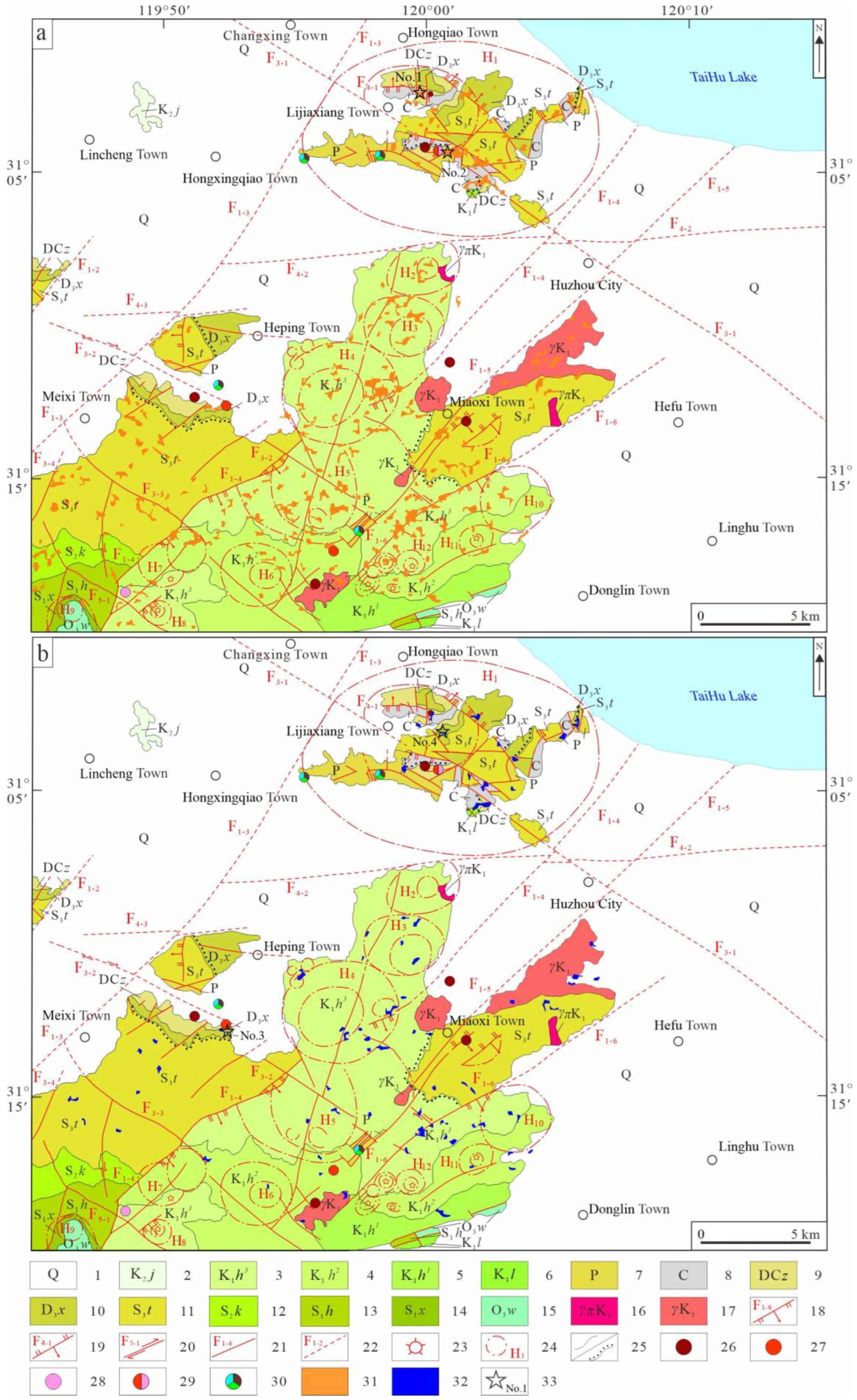
Among Fe-bearing alteration minerals, hematite exhibits distinct dual absorption features, with its first characteristic absorption trough located near 540 nm and its second near 880 nm. The spectral curve of pyrite lacks pronounced reflectance peaks, and its absorption troughs are relatively shallow; however, it still exhibits a dual-absorption features, with the first characteristic absorption trough located near 630 nm and the second near 840 nm. Based on the above spectral characteristics, the SAM algorithm was used to match the preprocessed hyperspectral data with the spectra of the target minerals, ultimately yielding distribution maps of hematite and pyrite alteration zones (Figure 12).

5.2. Extraction of Al-OH Type Alteration Minerals

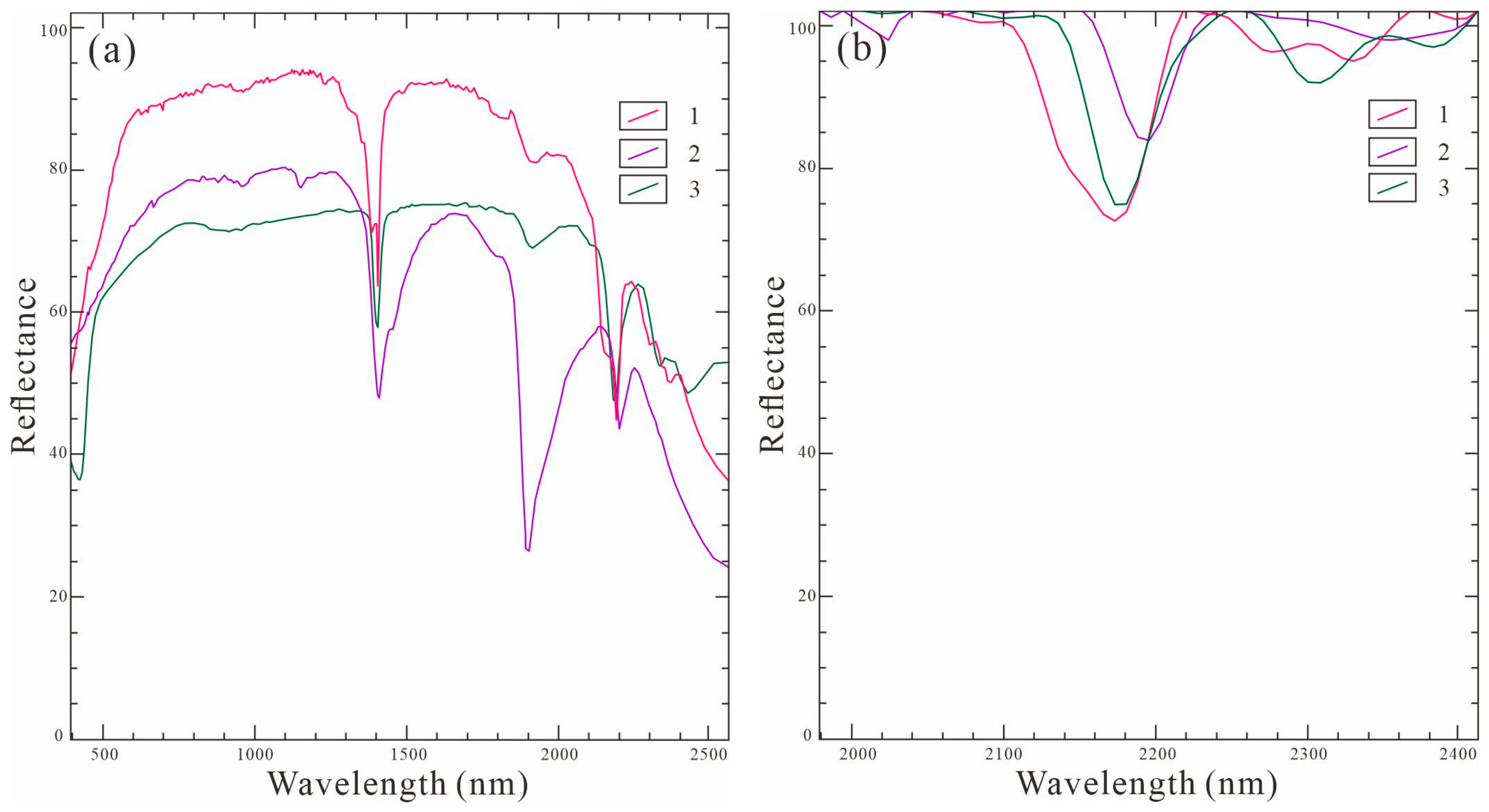
Analysis of the spectral curve characteristics reveals that the spectral features in the 1300–2500 nm range are primarily determined by CO₃²⁻, OH⁻, and H₂O in the mineral composition. Based on the major alteration mineral types in the study area and their spectral characteristics, kaolinite, montmorillonite, and muscovite were selected as target mineral spectra from the U.S. Geological Survey (USGS) standard spectral library (Figure 13a).

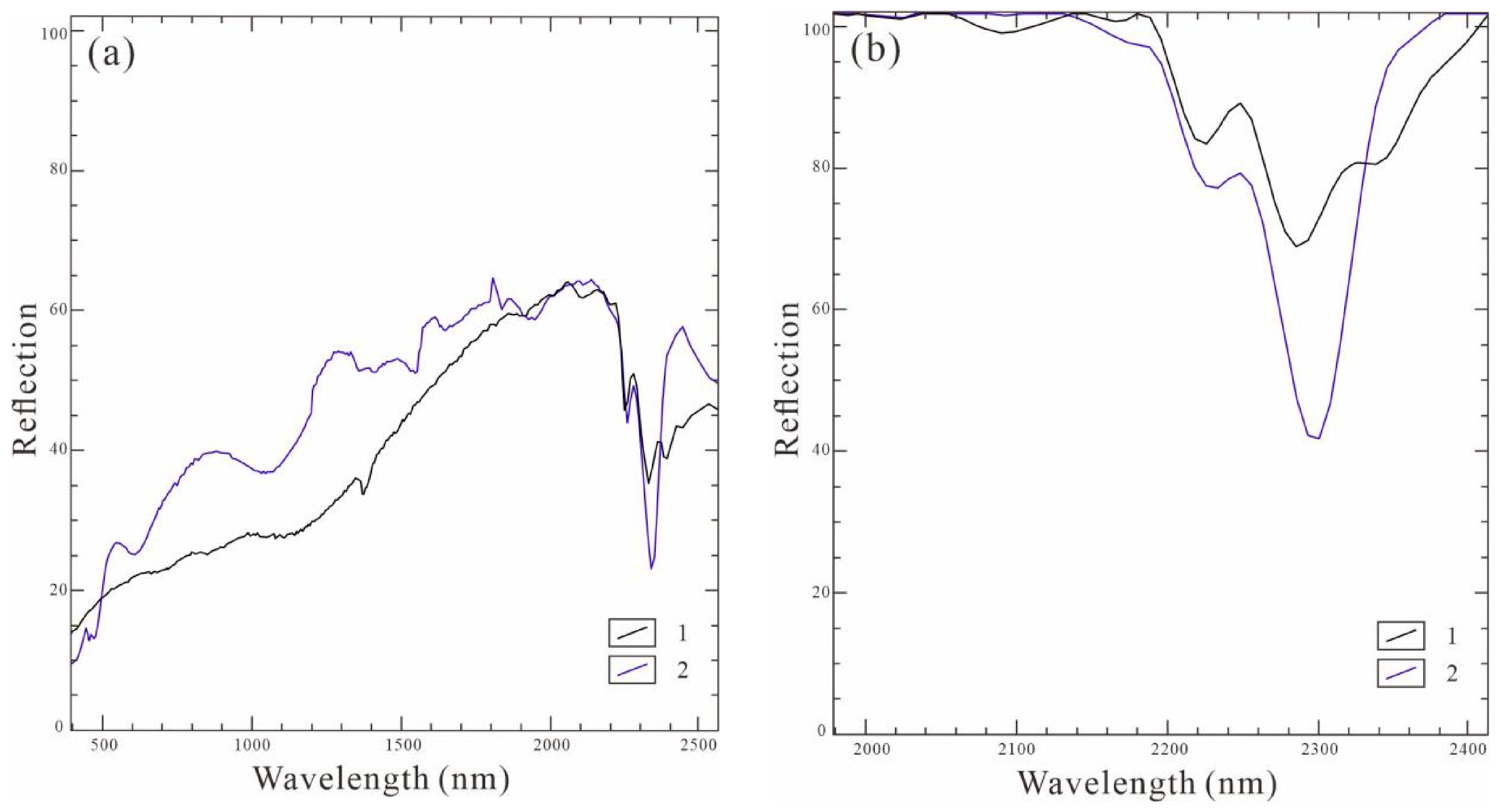
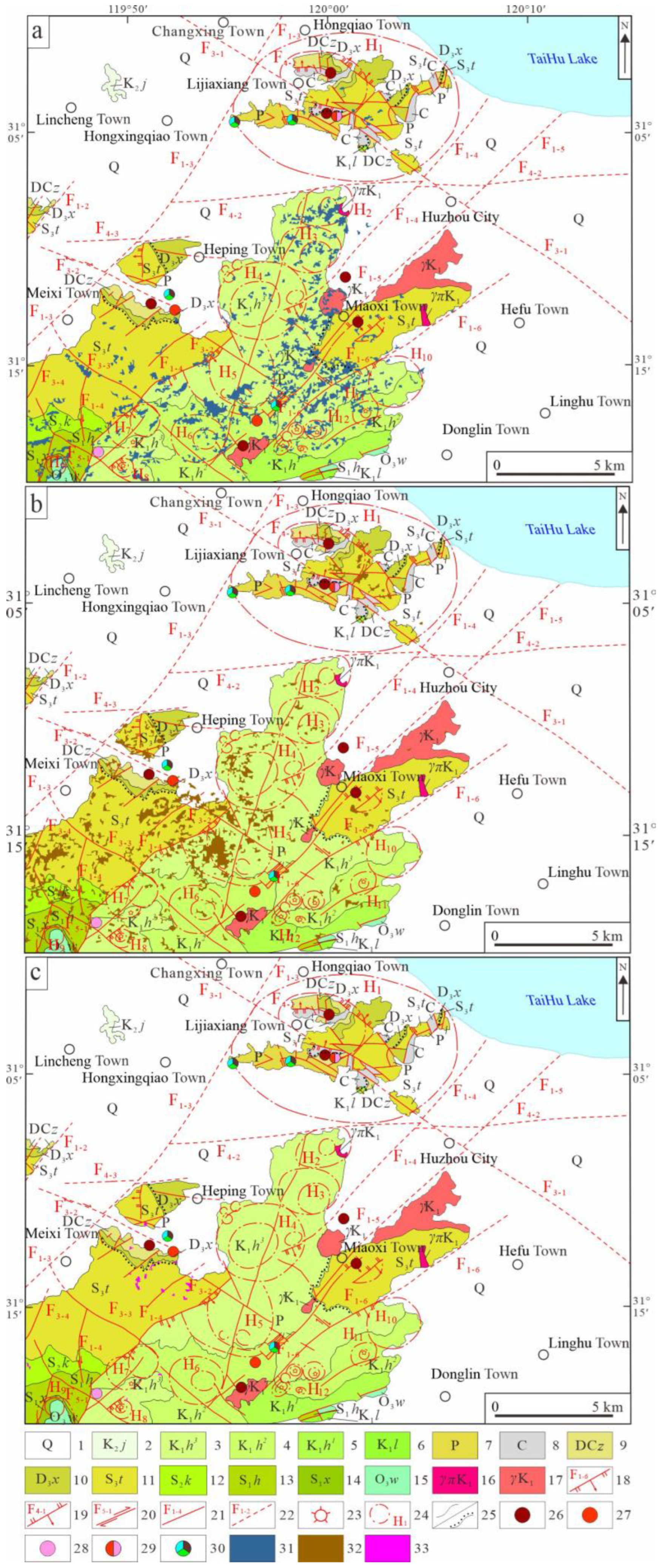
For Al-OH type alteration minerals, the diagnostic absorption trough is primarily located near 2200 nm. Therefore, for the GF-5B hyperspectral data, the wavelength range of 1976–2425 nm was selected as the spectral resampling interval, followed by Savitzky–Golay filtering and envelope removal (Figure 13b). Among Al-OH type alteration minerals, both kaolinite and montmorillonite exhibit distinct double absorption troughs, though their positions differ slightly, whereas muscovite has only one prominent absorption trough. The first characteristic absorption trough for both kaolinite and muscovite is located near 2195 nm, while that of montmorillonite is near 2220 nm. The positions of the second characteristic absorption troughs show significant differences: kaolinite is at 2372 nm, while montmorillonite is at 2397 nm. Based on these spectral characteristics, the SAM algorithm was used to match the preprocessed hyperspectral data with the spectra of the target minerals, ultimately yielding distribution maps of montmorillonite, muscovite, and kaolinite alteration zones in the study area (Figure 14).

5.3. Extraction of Mg-OH Type Alteration Minerals

Based on the dominant alteration mineral species and their diagnostic spectral signatures across the study area, chlorite and epidote were selected as target mineral spectra from the U.S. Geological Survey (USGS) standard spectral library (Figure 15a). The diagnostic absorption troughs of Mg-OH alteration minerals are primarily located near 2310 nm and 2330–2350 nm. Therefore, for the GF-5B hyperspectral data, the range of 1976–2425 nm was selected as the sensitive band range for spectral resampling, followed by Savitzky–Golay filtering, smoothing, and spectral envelope removal (Figure 15b).

Among Mg–OH alteration minerals, both chlorite and epidote exhibit only one distinct absorption trough, though their positions differ slightly. Specifically, the characteristic absorption trough of chlorite is located near 2254 nm, while that of epidote is near 2268 nm. Based on these spectral characteristics, the SAM algorithm was used to match the preprocessed hyperspectral data with the spectra of the target minerals, ultimately yielding distribution maps of chlorite and epidote alteration zones in the study area (Figure 16).

6. Discussion

6.1. Analysis of the Distribution Characteristics of Alteration Minerals

Utilizing SAM analysis from GF-5B hyperspectral imagery, hydrothermal alteration minerals were categorized into three genetically distinct groups: (1) Fe-bearing alteration minerals comprising hematite and pyrite; (2) Al-OH type alteration minerals comprising montmorillonite, kaolinite, and muscovite; and (3) Mg-OH type alteration minerals comprising chlorite and epidote. These three categories of alteration minerals exhibit distinct distribution patterns with clear boundaries, and their distribution characteristics are closely linked to lithological boundaries and fault structures. Integrated interpretation of alteration zoning maps and regional geology reveals that these minerals are generally distributed in concentrated bands and patches along the NE-trending main fault, at the contacts of intrusive bodies, and along the margins of volcanic basins.

(1)

Fe-bearing alteration minerals

The Fe-bearing alteration assemblages in the study area are primarily composed of hematite with subordinate quantities of pyrite. These mineralogical signatures exhibit predominant spatial distribution patterns along the northern segment of the F_3-1 strike-slip fault system and peripheral zones of the annular structure within the central–southern volcanic basin complex. The observed zonation patterns demonstrate pronounced spatial correlations with Au-Ag vein systems and polymetallic mineralization centers identified through field validation (Figure 12).

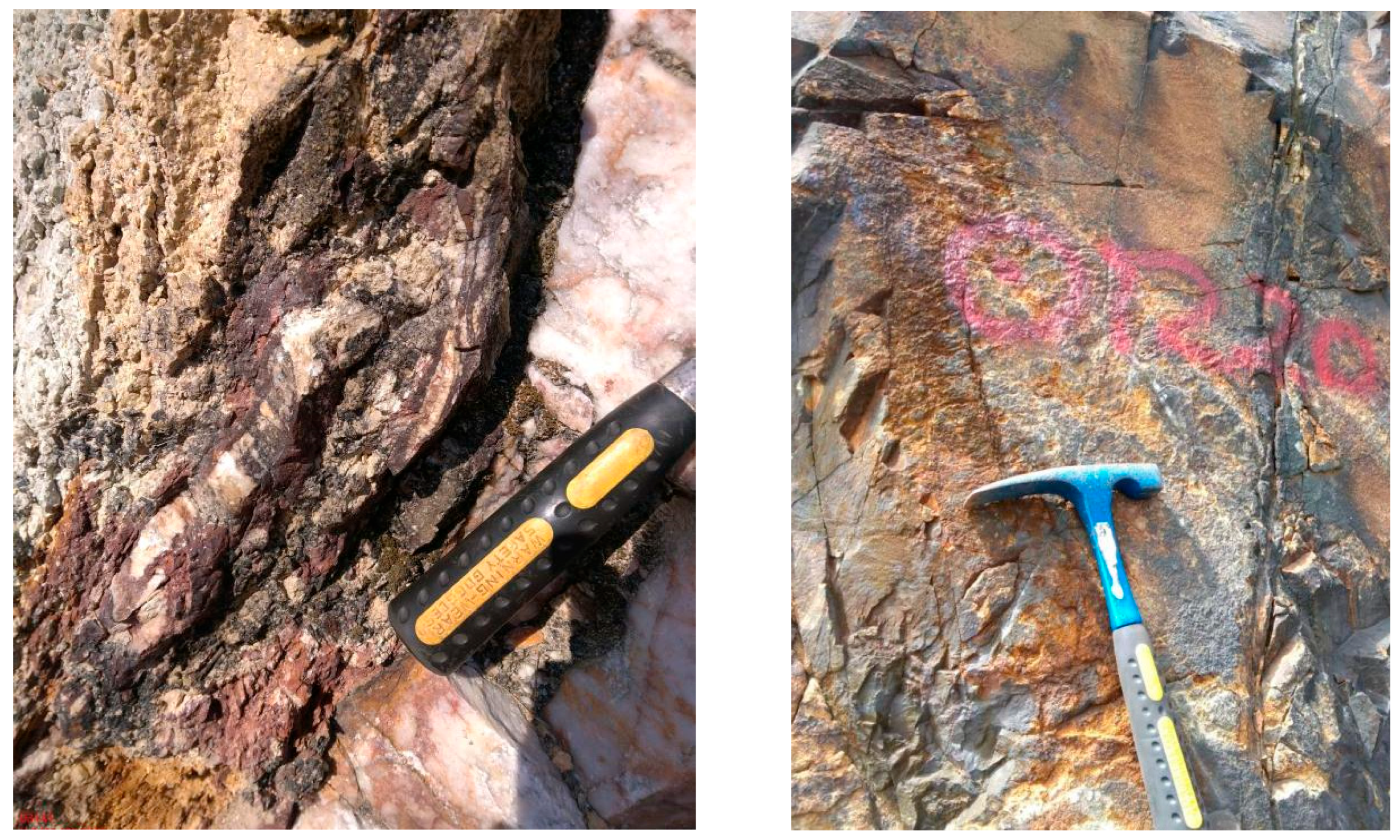
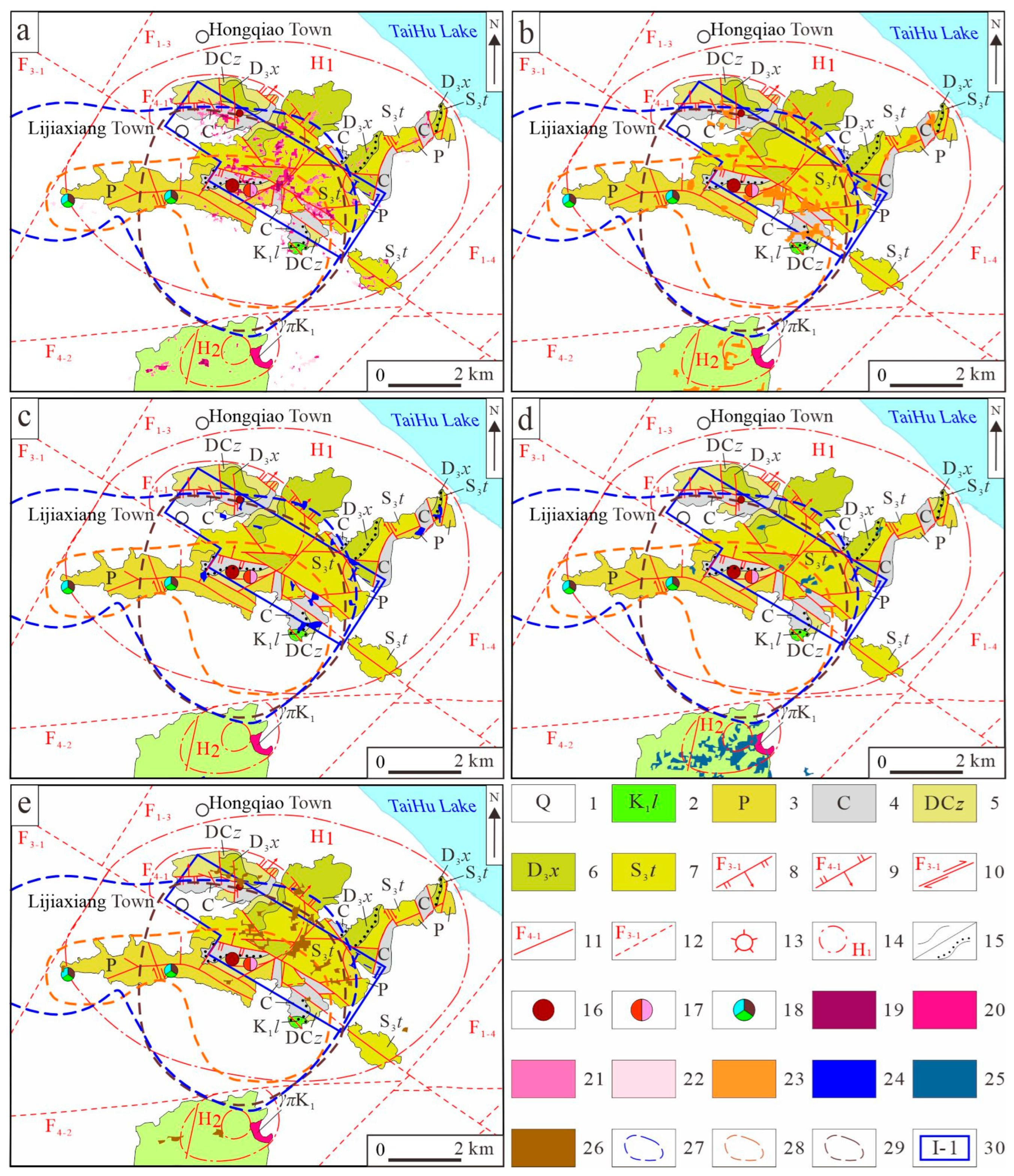
Hematite alteration exhibits predominant spatial distribution along the northern segment of the F_3-1 strike-slip fault system and peripheral annular fracture networks within the central–southern volcanic basin complex, manifesting as discontinuous concentric arrays. Significant concentration occurs in Lijiaxiang, Miaoxi, and Meixi townships, within the H₁, H₂, H_3, H₄, H₅, H₆ annular structures within the basin, and in the zones bounded by the F_1-5 and F_1-6 faults (Figure 12a and Figure 17).

Petrostratigraphic analysis reveals preferential enrichment of hematite alteration within Carboniferous Huanglong Formation platform carbonates (northern sector) and Cretaceous Huangjian Formation III-stage rheomorphic ignimbrites (central–southern sector), transitioning to discontinuous linear arrays where Silurian Tangjiawu Formation mature quartz arenites dominate the lithology.

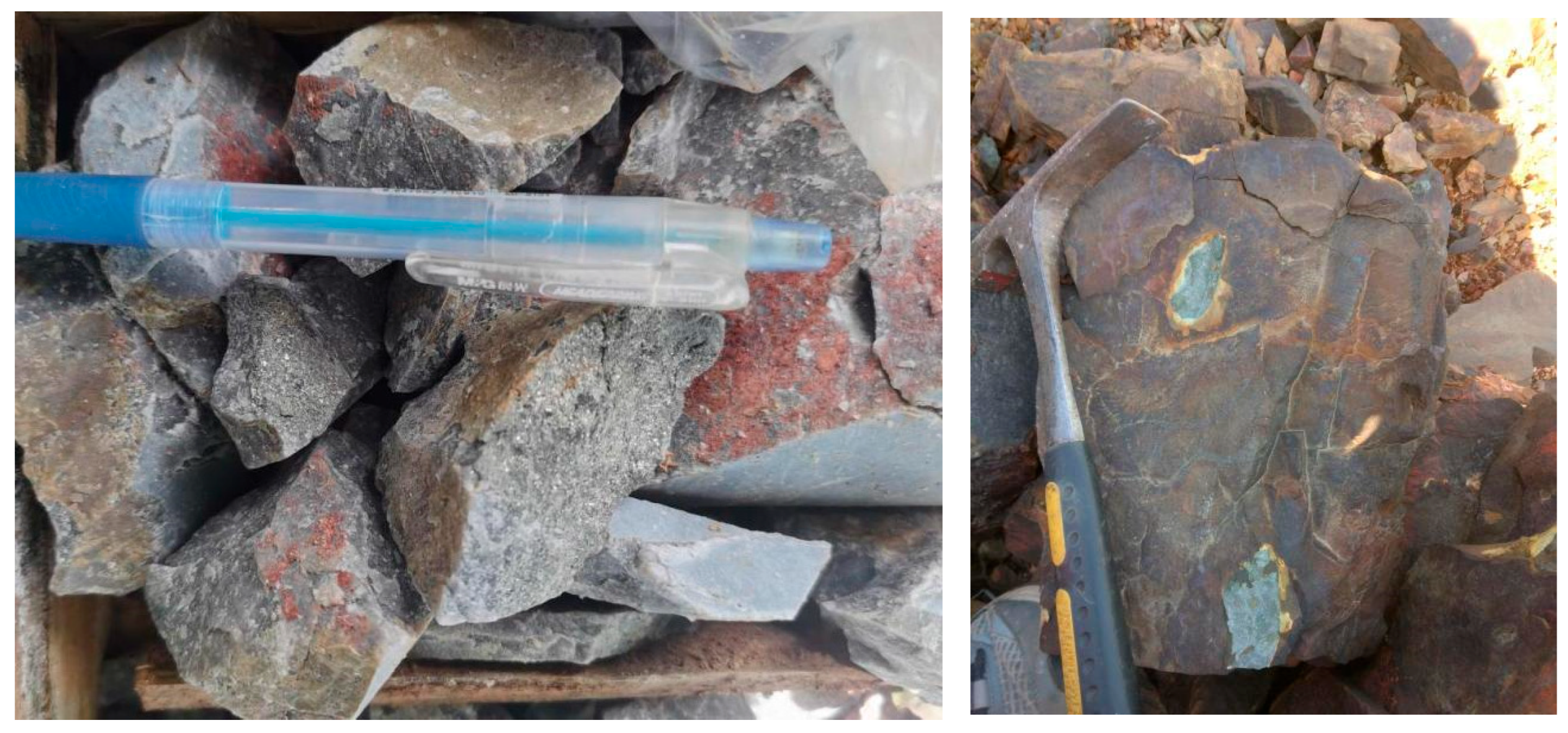
Pyrite alteration exhibits preferential localization along fault systems but demonstrates pronounced spatial sparsity, with individual altered zones exhibiting limited surface exposure extent (Figure 12b). The mineralization corridors align closely with the F_3-1 strike-slip fault system, occurring in small, patchy clusters near Li Jiaxiang Town, Meixi Town, and Heping Town within the annular structure of the Moganshan Volcanic Basin, as well as south of Miaoxi Town. Lithological targeting reveals maximal pyritization intensity within: biohermal bioclastic limestone sequences of the Carboniferous-Permian Chuanshan Formation (northern sector) and rheomorphic ignimbrites of the third member of the Cretaceous Huangjian Formation (central–southern sector). Secondary concentrations form concentric alteration aureoles around Early Cretaceous granodioritic plutons at Miaoxi Township contacts. Pyritic mineralization patterns exhibit dominant paragenetic styles characterized by disseminated grain distributions and sporadic nodular aggregates within host lithologies (Figure 18).

(2)

Al-OH type alteration minerals

Al–OH-type alteration assemblages are predominantly expressed as mineralogical transformations involving montmorillonite, muscovite, and kaolinite, with their spatial zonation patterns systematically governed by lithological heterogeneity, fault systems architecture, and intrusive contact aureoles.

Montmorillonite alteration exhibits predominant spatial distribution across the Moganshan Volcanic Basin, extending over large surface areas. Distinct concentration nuclei develop preferentially at intersections between the central annular structure and F_1-4, F_1-5, and F_1-6 fault systems, whereas limited occurrences are restricted to epithermal Au-Ag mineralization zones along the northern F_3-1 strike-slip fault corridor (Figure 14a). Lithological targeting reveals maximal montmorillonite development within rheomorphic ignimbrites of the Cretaceous Huangjian Formation, Silurian Xiashang Formation siltstones, and vitric tuffs of the Cretaceous Laocun Formation, where it exhibits pervasive halo-type zonation. Contrasting minimal expression occurs in Carboniferous-Permian Chuanshan Formation limestones and Carboniferous Huanglong Formation platform carbonates.

Unlike the diffuse spatial dispersion of montmorillonite alteration, both muscovite and kaolinite alterations demonstrate distinct structural confinement patterns. Muscovite alteration occurs in a patchy or banded pattern, concentrated at fault intersections and along the contact zones of intrusive bodies. Principal exposure loci include the NE-trending F_3-1 strike-slip fault nexus of Lijiaxiang Township and the peripheral metasomatic halo of the Miaoxi Early Cretaceous granodiorite pluton. This alteration type displays circumferential zonation constrained by the Moganshan caldera boundary faults, exhibiting progressive westward enrichment correlated with fracture density gradients (Figure 14b). Lithologically controlled sericitization predominates within rheomorphic ignimbrite breccias of the third member of the Cretaceous Huangjian Formation and Silurian Tangjiawu Formation quartz arenites, with subordinate occurrences in eastern volcaniclastic sequences.

Kaolinite alteration exhibits preferential concentration within intrusive contact aureoles, the western volcanic basin sector, and annular structures. Principal exposure loci occur along the Early Cretaceous granite and granite porphyry contact aureole at Miaoxi Township’s eastern margin. A small amount is also distributed near the NW-trending fault zone F_1-4 in the southwestern part of the study area (Figure 14c). Lithological targeting reveals primary enrichment within Silurian Tangjiawu Formation turbiditic successions (quartz arenite/siltstone/mudstone rhythmites). Secondary occurrences appear as discontinuous pods within rheomorphic ignimbrites of the Cretaceous Huangjian Formation and Silurian Helixi Formation distal shelf facies (siltstone-dominant heterolithics). Its distribution closely corresponds to the morphology of the intrusive bodies.

(3)

Mg-OH type alteration minerals

Mg–OH alteration assemblages are predominantly characterized by chloritization and epidotization processes, exhibiting distinct latitudinal zonation with preferential concentration in southern sectors relative to northern regions.

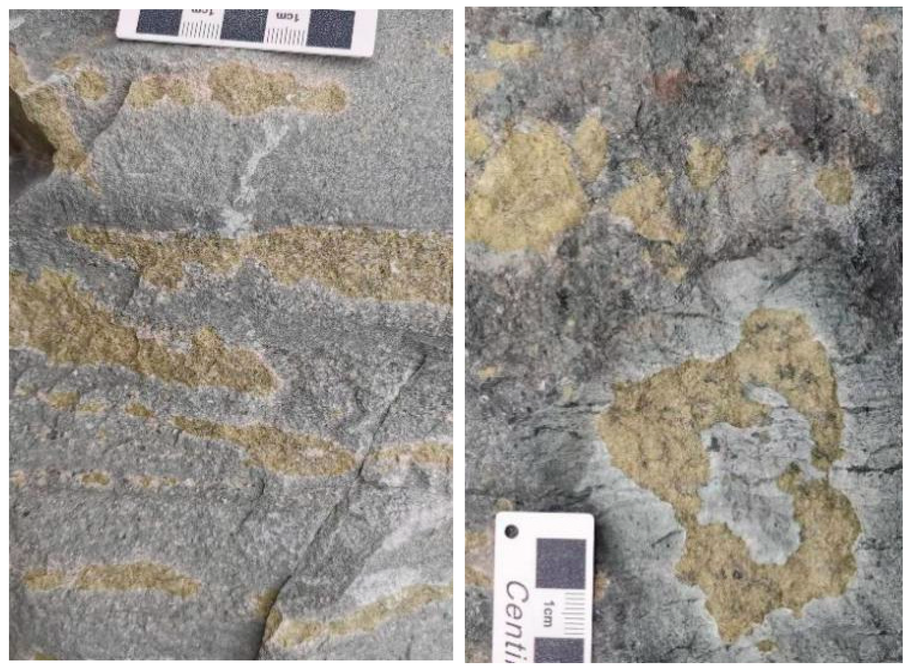
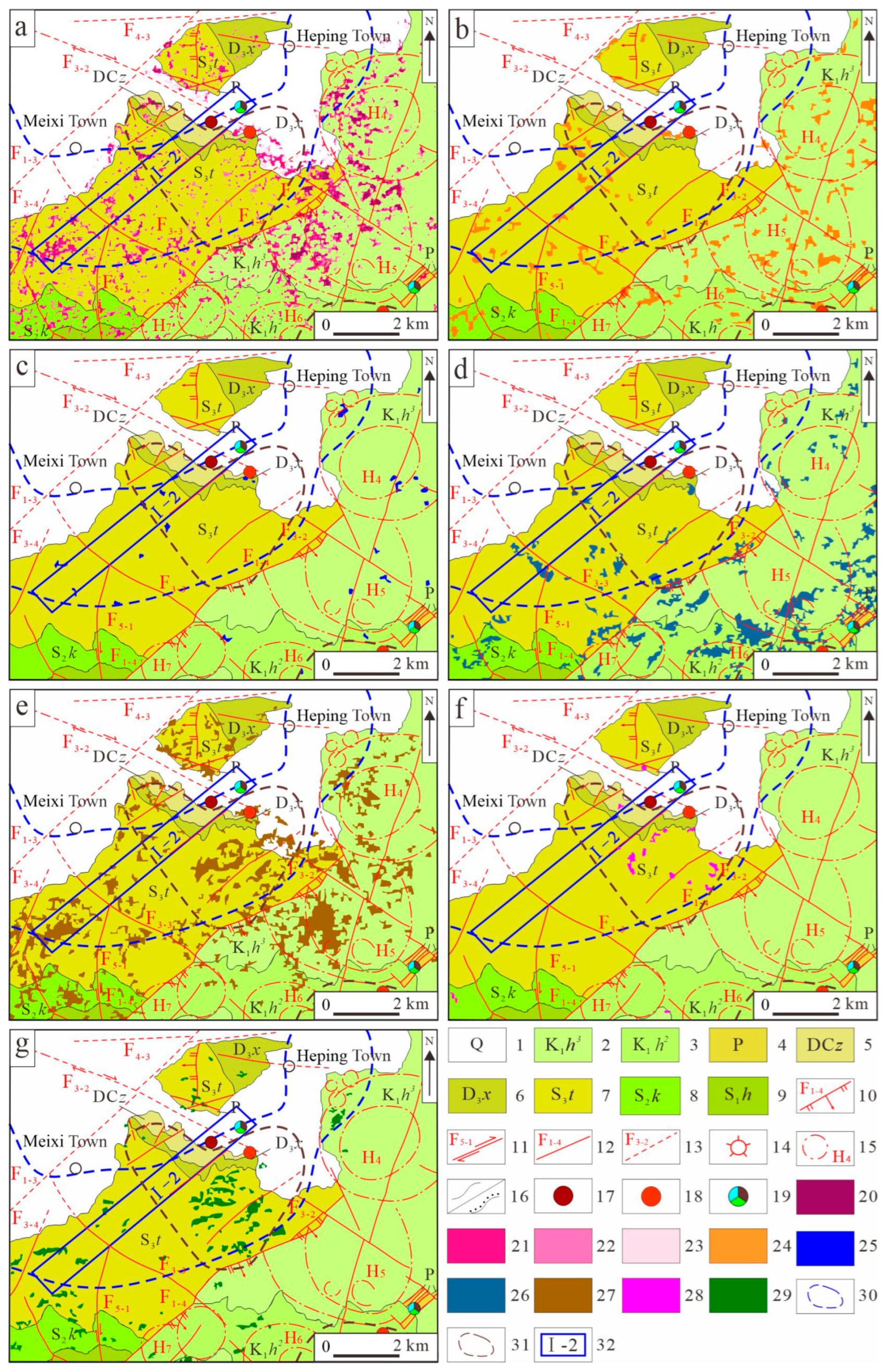
Chlorite alteration demonstrates pronounced development along the southwestern rim of the Moganshan Caldera Basin (SE Meixi Township), spatially correlating with lithostratigraphic contacts between the Silurian Kangshan Formation, Silurian Tangjiawu/Helixi Formations, and Jurassic Xiaxiang Group. It forms discontinuous lenticular arrays controlled by the F_1-4, F_3-4 and F_5-1 fault systems (Figure 16a), showing paragenetic association with garnet-bearing skarn assemblages at the Heping B-Pb-Zn ore system and reflecting polyphase hydrothermal overprinting. It predominantly manifests as millimeter-scale epigenetic veinlets and orbicular aggregates within the host rocks (Figure 19).

Epidote alteration is relatively limited, occurring as isolated exposures within southern Huzhou municipal boundaries. Structurally confined by F_1-5 and F_1-6 fault systems, it forms discontinuous podiform concentrations within their inter-fault domain proximal to lithostratigraphic interfaces between Silurian Tangjiawu Formation meta-sandstones comprising rhythmically interbedded siltstone and mudstone layers, and Early Cretaceous porphyritic granodiorite plutons (Figure 16b).

6.2. Prediction of Prospective Areas for Mineral Exploration

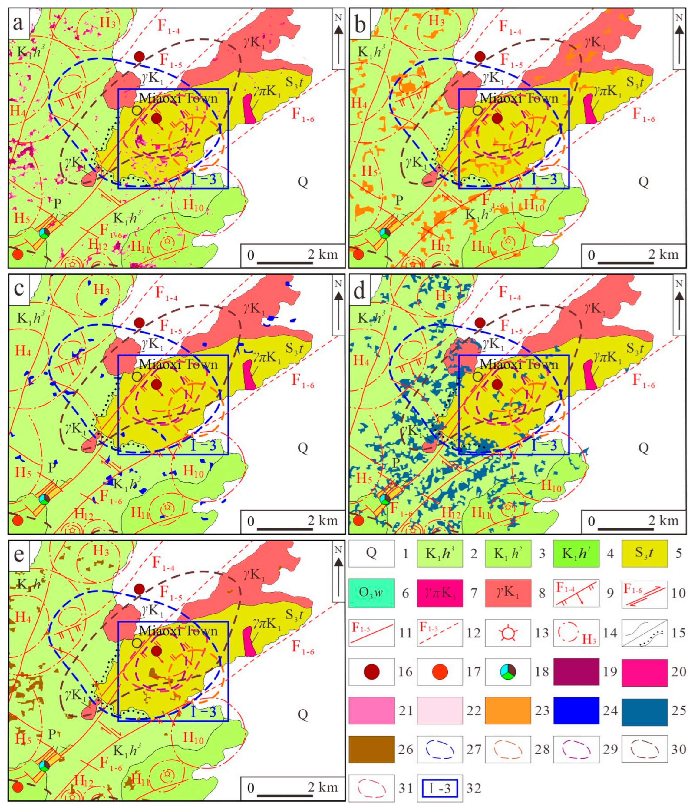
Through systematic analysis of alteration mineral distributions, including Fe-bearing phases (hematite, pyrite), Al-OH type phases (kaolinite, montmorillonite, muscovite), and Mg-OH type phases (chlorite, epidote), totaling seven distinct mineral species, we performed binary classification of spectral unmixing results. Pixel values were dichotomized (1 = alteration presence, 0 = absence), followed by weighted overlay analysis where individual mineral layers received domain-specific coefficients. Spatial coexistence analysis revealed maximum superposition of four alteration mineral types per pixel, enabling generation of a multigrade zonation map (Figure 20). Mineralogical abundance grading was defined as follows: Grade I (four concurrent minerals), Grade II (three minerals), Grade III (two minerals), and Grade IV (single mineral manifestation). Integration of multidisciplinary datasets, comprising mineralogical assemblages, curvilinear structural systems, lithostratigraphic units, known mineral occurrences, and geochemical anomalies, enabled the delineation of high-potential exploration targets (Figure 20).

The Lijiaxiang town prospective exploration area (I-1) is situated within the H₁ annular structural system in the northern study area and exhibits strong spatial correspondence with Fe, Au-Ag, and polymetallic deposits and occurrences (Figure 21). This zone demonstrates composite alteration assemblages comprising Fe-bearing phases and Al–OH-type mineralizations, predominantly developed in thick strata of the Tangjiawu Formation along the F_3-1 fault damage zone. The alteration is dominated by hematite–muscovite assemblages with pyrite-montmorillonite paragenesis, and subordinately occurs in the Huanglong, Chuanshan, Laohudong, and Xihu Formations. These alteration zones exhibit extensive distribution correlating with Au-Ag-Pb geochemical halos, demonstrating clear fault-controlled characteristics. Regional stratigraphy is dominated by Carboniferous Huanglong Formation carbonate rocks, offering optimal host lithologies for skarn-forming processes. The intrusive body apex vertically aligns with the exploration target zone center, showing high correlation with the annular structure’s genetic mechanism depicted in Figure 21. The composite alteration assemblages resemble those of the Dayinshan-type Au deposits in temporal–spatial association [67], indicating significant metallogenic potential.

The Meixi town northeastern prospective exploration area (I-2) exhibits NE–SW elongation and hosts Fe-dominated, Pb–Zn–Cu polymetallic mineralization in its northeastern sector (Figure 22). Alteration assemblages are predominantly characterized by Fe-bearing phases and Al–OH type mineralizations with subordinate Mg-OH type manifestations distributed discontinuously. Hematite–muscovite paragenesis forms discontinuous lenticular arrays controlled by the F_3-3 fault system, accompanied by pyrite, montmorillonite, kaolinite, and chlorite alteration, preferentially developed within Silurian meta-sandstone layers of the Tangjiawu Formation. This alteration suite demonstrates strong spatiotemporal association with skarn alteration halos from the regional Heping B–Pb–Zn ore system, and correlates significantly with Au–Pb geochemical halos exceeding regional background values.

The Miaoxi town prospective exploration area (I-3) is situated in the northeastern Moganshan Volcanic Basin (Figure 23) and develops along the regional F_1-6 fault system. This area hosts Fe deposits and occurrences with extensive Fe–Al–OH composite alteration zones. Alteration predominantly affects Silurian meta-sedimentary rocks of the Tangjiawu Formation, exhibiting diverse parageneses including hematite–montmorillonite assemblages forming stratabound layers, accompanied by disseminated pyrite-muscovite occurrences. In Cretaceous Huangjian Formation fault gouge zones, montmorillonite forms nodular concentrations, with minor quantities extending into Early Cretaceous granitic plutons. These alteration features demonstrate significant spatial association with Au–Ag–Cu–Pb–Zn geochemical halos. Subsurface Pb–Zn sulfide mineralization confirmed through drilling operations [72] supports the effectiveness and reliability of spectral alteration mapping for mineral exploration.

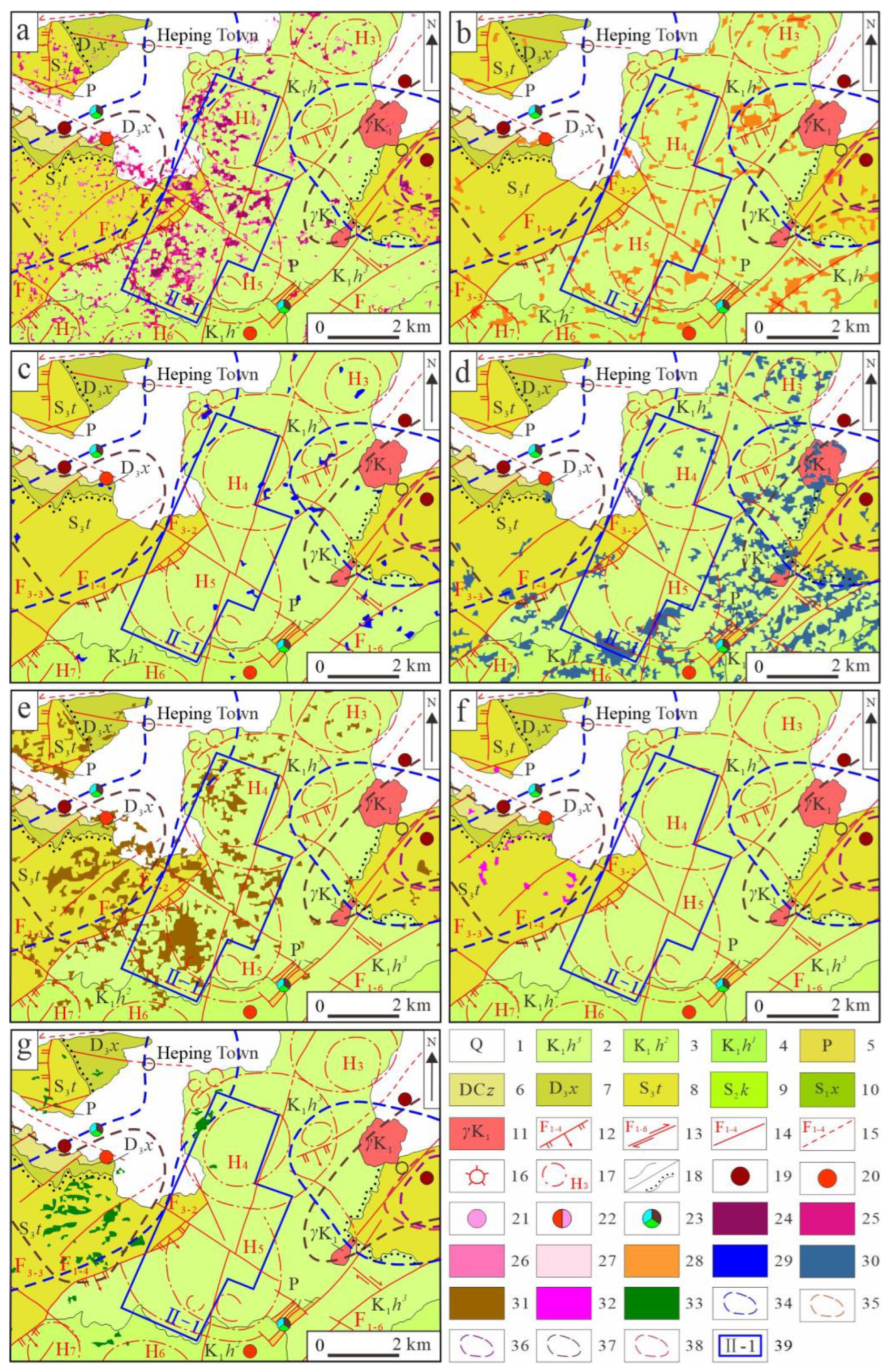
The central Moganshan volcanic basin prospective exploration area (II-1) is located at the intersection of a NE-trending main fault and a NW-trending secondary fault (Figure 24). An enrichment zone has formed at the intersection of the annular structures H₄ and H₅ with faults F_2-1, F_1-4, and F_3-2 in the central part of the volcanic basin. Iron, gold, and polymetallic deposits and occurrences are distributed around this prospective exploration area. The zone exhibits superimposed anomalies of Fe-bearing and Al–OH-type alteration minerals, occurring within the fractured and brecciated zones of the rhyolitic brecciated tuff of the third member of the Huangjian Formation in the Cretaceous System. Among these, muscovite alteration exhibits the widest areal distribution, followed by hematite alteration; montmorillonite, kaolinite, and chlorite alterations are also widely distributed, while pyrite alteration occurs sporadically, indicating characteristics of multi-phase superimposed hydrothermal mineralization. These alteration zones are jointly controlled by contact zone structures and fault systems. The deposit types are primarily hydrothermal filling, alteration-type, and skarn-type, predominantly occurring in fracture zones, fissure zones, and interlayer fracture zones within and around the contact zones of intermediate to acidic intrusions, exhibiting multi-level and multi-lithological characteristics. Multiple instances of copper–lead–zinc polymetallic mineralization have been identified in the area. Overall, the area demonstrates strong exploration potential for Cu–Pb–Zn polymetallic deposits.

6.3. Methodology Evaluation and Discussion

The main workflow for mapping alteration minerals comprises three key steps: basic image preprocessing, Zonal Adaptive Vegetation Suppression Technique (ZAVST), and interference masking. Among these, the ZAVST is based on the core concept of separating the spectral contributions of vegetation. By constructing a piecewise statistical relationship model between reflectance and the Normalized Difference Vegetation Index (NDVI), it quantitatively removes the spectral contributions of the vegetation component. This processing inevitably alters the reflectance values of the original pixels, which may potentially affect the accuracy of subsequent alteration mineral identification based on the Spectral Angle Mapper (SAM) method. Theoretically, changes in reflectance amplitude may interfere with SAM’s ability to distinguish diagnostic absorption features during spectral shape matching, thereby affecting the accuracy and reliability of mineral classification. Therefore, it is necessary to systematically evaluate and discuss the errors that this technique may introduce and their specific impact on classification accuracy.

To evaluate the reliability of the SAM classification results, this study conducted statistical validation of the classified images. Taking hematite as an example, statistical analysis showed that the mean spectral angle of the classified images of hematite in the study area was 0.6771. Within the prospective exploration area (I-1) in Lijiaxiang Town, regions of interest (ROIs) were selected near known iron ore occurrences and mineralized alteration zones, and the mean spectral angle of the corresponding pixels was 0.2423; within the prospective exploration area (I-2) in the eastern part of Meixi Town, the mean spectral angle of the corresponding pixels was 0.2627; within the prospective exploration area (I-3) in Miaoxi Town, the mean spectral angle of the corresponding pixels was 0.2696; and within the prospective exploration area (II-1) in the central part of the Moganshan Volcanic Basin, the mean spectral angle of the corresponding pixels was 0.2754. These results indicate that the mean spectral angles in the high-confidence areas identified by SAM are significantly lower and show a high degree of correlation with the spatial locations of known mineralization, thereby validating the reliability of the alteration mineral extraction results obtained in this study.

7. Conclusions

(1)

To tackle the technical challenges posed by dense vegetation cover and weak spectral responses of alteration minerals in Huzhou, Zhejiang Province, China, we propose a zone-based adaptive vegetation suppression method incorporating piecewise spectral–statistical modeling. Developed through establishing segmented statistical correlations between multi-band reflectance characteristics and NDVI values, this technique demonstrates superior capability in suppressing vegetation masking effects while preserving diagnostic absorption features of subsurface alteration minerals, enhancing alteration mineral detection accuracy compared to traditional methods under equivalent vegetated conditions. The proposed methodology has been rigorously validated through field sampling and hyperspectral core scanning datasets from the study area.

(2)

Utilizing the Advanced Hyperspectral Imager (AHSI) onboard China’s GF–5B satellite combined with the Spectral Angle Mapper (SAM) algorithm, we systematically identified seven distinct alteration mineral species grouped into three genetic categories within the Moganshan volcanic basin: Fe-bearing alteration phases (hematite, pyrite), Al–OH alteration assemblages (kaolinite, montmorillonite, muscovite), and Mg–OH type alteration associations (chlorite, epidote). Spatial analysis reveals that Fe-bearing phases exhibit predominant alignment with NE-striking fault systems and Mesozoic volcanic basin boundaries, while Al–OH-dominated assemblages show preferential development in metasomatic aureoles surrounding Cretaceous granitoid plutons. Notably, Mg–OH-associated minerals demonstrate pronounced concentration at interfaces between Paleozoic carbonate platforms and concealed granitic intrusions. These spatial correlations underscore the decisive control exerted by syn-magmatic faulting episodes and multi-stage hydrothermal fluid circulation on alteration zonation patterns.

(3)

Analysis of alteration mineral superimposition revealed anomalous zones characterized by the coexistence of up to four types of alteration minerals across the study area. Spatial clustering occurs predominantly at NE-trending and NW-trending fault intersections, along intrusive contact zones, and within annular structural margins, demonstrating strong tectonic-magmatic control. Combined with the spatial distribution characteristics of known deposits and occurrences, this confirms that zones with superimposed alteration minerals of multiple types are highly correlated with mineralization and can serve as important indicators for mineral exploration in this study area.

(4)

Through systematic integration of multi-source exploration datasets including alteration mineral assemblages, characteristics of lineament and annular structures, lithostratigraphic units, and geochemical element anomalies, four priority mineral exploration targets were delineated: Lijiaxiang Town, eastern Meixi Town, Miaoxi Town, and the central Moganshan Volcanic Basin.

The highest priority target zone (I-1) at Lijiaxiang Town exhibits intense spatial superposition of Fe-bearing and Al–OH alteration phases, manifesting as massive concentrated zones along the margins of the F_3-1 fault and within H₁ annular structure boundaries. This alteration zonation demonstrates robust spatial correspondence with concealed granitic plutons and Cretaceous volcanic-intrusive interface zones. The prospective exploration area (I-2) in the eastern part of Meixi Town exhibits extensive anomalies of Fe-bearing and Al–OH-type alteration minerals, accompanied by sporadically distributed Mg–OH-type alteration minerals; the host rock alteration shows good correlation with gold and lead geochemical anomalies. The prospective exploration area (I-3) in Miaoxi Town is located in the northeastern part of the Moganshan Volcanic Basin, extending along the F_1-6 fault. It exhibits Fe-bearing alteration and Al–OH-type alteration, strongly associated with Au–Ag–Cu–Pb–Zn geochemical trains. The prospective exploration area (II-1) in the central part of the Moganshan Volcanic Basin exhibits superimposed hydrothermal alteration from multiple stages. Its spatial location highly coincides with known lead-zinc polymetallic deposits and occurrences, indicating good potential for lead-zinc polymetallic mineral exploration.

References

1. Carranza, E.J.M.; Hale, M. Mineral imaging with Landsat Thematic Mapper data for hydrothermal alteration mapping in heavily vegetated terrane. Int. J. Remote Sens. 2002, 23, 4827–4852. [Google Scholar] [CrossRef]
2. Crosta, A.P.; De Souza Filho, C.R.; Azevedo, F.; Brodie, C. Targeting key alteration minerals in epithermal deposits in Patagonia, Argentina, using ASTER imagery and principal component analysis. Int. J. Remote Sens. 2003, 24, 4233–4240. [Google Scholar] [CrossRef]
3. Alimohammadi, M.; Alirezaei, S.; Kontak, D.J. Application of ASTER data for exploration of porphyry copper deposits: A case study of Daraloo–Sarmeshk area, southern part of the Kerman copper belt, Iran. Ore Geol. Rev. 2015, 70, 290–304. [Google Scholar] [CrossRef]
4. Gabr, S.S.; Hassan, S.M.; Sadek, M.F. Prospecting for new gold-bearing alteration zones at El-Hoteib area, South Eastern Desert, Egypt, using remote sensing data analysis. Ore Geol. Rev. 2015, 71, 1–13. [Google Scholar] [CrossRef]
5. Bodeving, S.; Vasyukova, O.V.; Williams-Jones, A.E. Controls on the origin and evolution of wall-rock alteration at the Big Whopper Li-Cs-Ta pegmatite, Canada. Econ. Geol. 2025, 120, 689–714. [Google Scholar] [CrossRef]
6. Liu, J.G.; Li, Z.Y.; Zhang, W.L.; Nie, J.T. Evolution of ore-forming fluids in the deep polymetallic mineralization in western Xiangshan uranium ore field, Jiangxi Province: Evidence from altered wall rocks. Acta Geol. Sin. 2026, 100, 202–222. [Google Scholar] [CrossRef]
7. Cardoso-Fernandes, J.; Teodoro, A.C.; Lima, A. Remote sensing data in lithium (Li) exploration: A new approach for the detection of Li-bearing pegmatites. Int. J. Appl. Earth Obs. Geoinf. 2019, 76, 10–25. [Google Scholar] [CrossRef]
8. Du, X.C.; Lou, D.B.; Zhang, C.Q.; Xu, L.G.; Liu, H.; Fan, Y.L.; Zhang, L.; Hu, J.M.; Li, B. Study on extraction of alteration information from GF-5, Landsat8 and GF-2 remote sensing data: A case study of Ningnan lead-zinc ore concentration area in Sichuan Province. Miner. Depos. 2022, 41, 839–858. [Google Scholar] [CrossRef]
9. Shirmard, H.; Farahbakhsh, E.; Müller, R.D.; Chandra, R. A review of machine learning in processing remote sensing data for mineral exploration. Remote Sens. Environ. 2022, 268, 112750. [Google Scholar] [CrossRef]
10. Ivanova, Y.N. Predicting promising areas for gold ore mineralization based on the integration of geological and geophysical information and processing the data set of the Harmonized Landsat Sentinel-2 remote sensing space vehicle for the northern end of the eastern slope of the Polar Urals. Izv. Atmos. Ocean. Phys. 2024, 60, 1579–1596. [Google Scholar] [CrossRef]
11. Zhang, C.Y.; Huang, S.L.; Zhang, B.W.; Shen, Y.Q.; Yalikun, Y.; Wang, J.N.; Shang, Y.Z. Mineral prospectivity mapping based on remote sensing and machine learning in the Hatu area, China. Minerals 2026, 16, 144. [Google Scholar] [CrossRef]
12. Crosta, A.P.; Sabine, C.; Taranik, J.V. Hydrothermal alteration mapping at Bodie, California, using AVIRIS hyperspectral data. Remote Sens. Environ. 1998, 65, 309–319. [Google Scholar] [CrossRef]
13. Wu, Z.C.; Hu, R.Q.; Guo, F.S.; Liu, L.Q.; Xie, C.F.; Jiang, Y.B.; Zhou, W.P. The extraction of alteration anomaly with remote sensing image of vegetation covered area in Xiangshan uranium field, Jiangxi Province. J. East China Univ. Technol. (Nat. Sci.) 2013, 29, 112–118, 85. [Google Scholar] [CrossRef]
14. Wambo, J.D.T.; Pour, A.B.; Ganno, S.; Asimow, P.D.; Zoheir, B.; Salles, R.D.R.; Nzenti, J.P.; Pradhan, B.; Muslim, A.M. Identifying high potential zones of gold mineralization in a sub-tropical region using Landsat-8 and ASTER remote sensing data: A case study of the Ngoura-Colomines goldfield, eastern Cameroon. Ore Geol. Rev. 2020, 122, 103530. [Google Scholar] [CrossRef]
15. Zhu, Y.D.; Wu, Z.C.; Ma, F.L.; Li, H.L.; Qin, Y.Z. Remote sensing interpretation of alteration anomaly based on fractal theory: A case study of Yangshan County, Guangdong Province. S. China Geol. 2024, 40, 380–392. [Google Scholar] [CrossRef]
16. Yuan, L.F.; Wu, Z.C.; Xu, Z.; Huang, J.; Li, H.L.; Zhang, Z.Q.; Jiang, H.; Yan, Z.W.; Huang, Y.F.; Jin, W. Remote sensing interpretation of surface linear-ring structures and wall-rock alteration in the Lingshan area, Shangrao City, Jiangxi Province, China: Implications for mineral prospecting. Geocarto Int. 2025, 40, 2584954. [Google Scholar] [CrossRef]
17. Zhu, Y.D.; Wu, Z.C. A synergistic PCA and CA fractal approach for high-precision extraction of mineral alteration anomalies from ASTER remote sensing data. Geocarto Int. 2025, 40, 2476599. [Google Scholar] [CrossRef]
18. Dong, X.F.; Gan, F.P.; Li, N.; Yan, B.K.; Zhang, L.; Zhao, J.Q.; Yu, J.C.; Liu, R.Y.; Ma, Y.N. Fine mineral identification of GF-5 hyperspectral image. J. Remote Sens. 2020, 24, 454–464. [Google Scholar] [CrossRef]
19. Bai, L.Y.; Dai, J.J.; Wang, N.; Li, B.L.; Liu, Z.B.; Li, Z.J.; Chen, W. Extraction of mineral alteration information and mineralization prospecting analysis based on GF-5 hyperspectral in Zhule-Mangla, Tibet. Geol. China 2024, 51, 995–1007. [Google Scholar] [CrossRef]
20. Feng, X.H.; Huang, J.J.; Chen, X.M.; Zhou, H.; Zhang, M.; Zhang, C.; Ye, F.W. Research on hyperspectral remote sensing alteration mineral mapping using an improved ViT model. Comput. Geosci. 2025, 206, 106037. [Google Scholar] [CrossRef]
21. Habashi, J.; Pour, A.B.; Muslim, A.M.; Afrapoli, A.M.; Hong, J.K.; Park, Y.; Almasi, A.; Crispini, L.; Hashim, M.; Bagheri, M. Revealing critical mineralogical insights in extreme environments using deep learning technique on hyperspectral PRISMA satellite imagery: Dry Valleys, South Victoria Land, Antarctica. ISPRS J. Photogramm. Remote Sens. 2025, 228, 83–121. [Google Scholar] [CrossRef]
22. Ramadan, T.M.; Abdelsalam, M.G.; Stern, R.J. Mapping gold-bearing massive sulfide deposits in the Neoproterozoic Allaqi Suture, Southeast Egypt with Landsat TM and SIR-C/X SAR images. Photogramm. Eng. Remote Sens. 2001, 67, 491–498. [Google Scholar]
23. Cheng, Y.; Tong, L.Q. The research on model of the alteration mineral mapping based on multi-level separate background and an application examples. Remote Sens. Technol. Appl. 2015, 30, 586–591. [Google Scholar]
24. Zhao, H.S.; Bruzzone, L.; Guan, R.C.; Zhou, F.F.; Yang, C. Spectral-spatial genetic algorithm-based unsupervised band selection for hyperspectral image classification. IEEE Trans. Geosci. Remote Sens. 2021, 59, 9616–9632. [Google Scholar] [CrossRef]
25. Maurya, K.; Mahajan, S. Mangrove species discrimination using modified spectral angle mapper algorithm on hyperspectral imagery: A study at Marine National Park (MNP) Jamnagar, Gulf of Kutch, Gujarat and Lothian Island, Sundarbans, West Bengal. Expert Syst. Appl. 2024, 237, 121455. [Google Scholar] [CrossRef]
26. Ng-Cutipa, W.L.; Lobato, A.; González, F.J.; Georgalas, G.P.; Zananiri, I.; Carvalho, M.; Teodoro, A.C. Spectral angle mapper application using Sentinel-2 in coastal placer deposits in Vigo Estuary, Northwest Spain. Remote Sens. 2025, 17, 1824. [Google Scholar] [CrossRef]
27. Dai, X.J.; Nie, F.; Dong, H.; Zou, J.Z.; Hu, X.X.; Li, J.; Wang, Y.C.; Lei, D.; Li, J.; Yao, B. Multi-source remote sensing geological interpretation and alteration information extraction in the Dechang area, Panxi Rift Zone. Sediment. Geol. Tethyan Geol. 2025, 45, 833–845. [Google Scholar] [CrossRef]
28. Wu, W.X.; He, L.; Zhao, J.K.; He, Z.W.; Chen, X.; Gong, J.S.; Que, Y.Q. Alteration mineral mapping and thermal anomaly reconstruction based on GF-5 data: A case study of the Ga’erqiong-Galale Cu-Au mining district, Tibet. Ore Geol. Rev. 2026, 190, 107185. [Google Scholar] [CrossRef]
29. Zhang, E.; Zhang, X.R.; Yang, S.Y.; Wang, S. Improving hyperspectral image classification using spectral information divergence. IEEE Geosci. Remote Sens. Lett. 2013, 11, 249–253. [Google Scholar] [CrossRef]
30. Rao, D.A.; Guha, A. Potential utility of spectral angle mapper and spectral information divergence methods for mapping lower Vindhyan rocks and their accuracy assessment with respect to conventional lithological map in Jharkhand, India. J. Indian Soc. Remote Sens. 2018, 46, 737–747. [Google Scholar] [CrossRef]
31. Chen, Q.; Cai, D.Y.; Xia, J.S.; Zeng, M.; Yang, H.Y.; Zhang, R.S.; He, Y.; Zhang, X.X.; Chen, Y.; Xu, X.H.; et al. Remote sensing identification of hydrothermal alteration minerals in the Duobuza porphyry copper mining area in Tibet using WorldView-3 and GF-5 data: The impact of spatial and spectral resolution. Ore Geol. Rev. 2025, 180, 106573. [Google Scholar] [CrossRef]
32. Saeidan, A.; Caulfield, J.; Vuts, J.; Yang, N.; Fisk, I. Detection of aphid infestation on faba bean (Vicia faba L.) by hyperspectral imaging and spectral information divergence methods. J. Plant Dis. Prot. 2025, 132, 109. [Google Scholar] [CrossRef] [PubMed]
33. Demšar, U.; Harris, P.; Brunsdon, C.; Fotheringham, A.S.; McLoone, S. Principal component analysis on spatial data: An overview. Ann. Assoc. Am. Geogr. 2013, 103, 106–128. [Google Scholar] [CrossRef]
34. Han, H.H.; Wang, Y.L.; Zhang, Z.; Li, J.Q.; Gao, T. Extraction and analysis of remote sensing alteration anomaly at shallow loess covering area in East Kunlun. Remote Sens. Land Resour. 2018, 30, 72–79. [Google Scholar] [CrossRef]
35. Zhang, K.; Ma, S.B.; Li, G.J.; Li, D.L.; Liu, S.Y. Ore prediction based on remote sensing data from Chinese-made satellite: Taking northern border of Qaidam as an example. Remote Sens. Land Resour. 2019, 31, 58–68. [Google Scholar] [CrossRef]
36. Wu, Z.C.; Guo, F.S.; Li, H.L.; Xu, H.; Zhang, S.M.; Li, G.R.; Zhang, W.L.; Zhu, M.Q. Application of principal component analysis in interpretation of alteration zone in the Xiangshan volcanic basin. Geotecton. Metallog. 2020, 44, 385–403. [Google Scholar] [CrossRef]
37. El-Wardany, R.; Jiao, J.G.; Zoheir, B.; Khedr, L.; Kumral, M.; Liu, L.; Abu El-Leil, I.; Orabi, A.; Abd El-Salam, L.; Abdelnasser, A. Remote sensing-based machine learning techniques for mapping gold-mineralized alteration zones in the Fatira mine area, Egypt. Acta Geol. Sin.-Engl. Ed. 2025, 99, 1196–1223. [Google Scholar] [CrossRef]
38. Zhang, C.; Ye, F.W.; Xu, Q.J.; Liu, H.C.; Meng, S. Mineral mapping and analysis of alteration characteristics using airborne hyperspectral remote sensing data in the Baiyanghe uranium and beryllium ore district, Xinjiang. Remote Sens. Land Resour. 2017, 29, 160–166. [Google Scholar] [CrossRef]
39. Fereydooni, H.; Mojeddifar, S. A directed matched filtering algorithm (DMF) for discriminating hydrothermal alteration zones using the ASTER remote sensing data. Int. J. Appl. Earth Obs. Geoinf. 2017, 61, 1–13. [Google Scholar] [CrossRef]
40. Fereydooni, H.; Moradzadeh, A.; Pahlavani, P.; Mojeddifar, S. Full unmixing hydrothermal alteration minerals mapping by integration of pattern recognition network and directed matched filtering algorithm. Earth Sci. Inform. 2020, 13, 417–431. [Google Scholar] [CrossRef]
41. Zadeh, M.H.; Tangestani, M.H.; Roldan, F.V.; Yusta, I. Mineral exploration and alteration zone mapping using mixture tuned matched filtering approach on ASTER data at the central part of Dehaj-Sarduiyeh copper belt, SE Iran. IEEE J. Sel. Top. Appl. Earth Obs. Remote Sens. 2013, 7, 284–289. [Google Scholar] [CrossRef]
42. Calin, M.A.; Coman, T.; Parasca, S.V.; Bercaru, N.; Savastru, R.; Manea, D. Hyperspectral imaging-based wound analysis using mixture-tuned matched filtering classification method. J. Biomed. Opt. 2015, 20, 046004. [Google Scholar] [CrossRef] [PubMed]
43. Wang, J.J.; Zhou, G.S.; Zhang, Y.; Bussink, C.; Zhang, J.H.; Ge, H. An unsupervised mixture-tuned matched filtering-based method for the remote sensing of opium poppy fields using EO-1 Hyperion data: An example from Helmand, Afghanistan. Remote Sens. Lett. 2016, 7, 945–954. [Google Scholar] [CrossRef]
44. Routh, D.; Seegmiller, L.; Bettigole, C.; Kuhn, C.; Oliver, C.D.; Glick, H.B. Improving the reliability of mixture tuned matched filtering remote sensing classification results using supervised learning algorithms and cross-validation. Remote Sens. 2018, 10, 1675. [Google Scholar] [CrossRef]
45. Du, H.Q.; Jin, W.; Ge, H.L.; Fan, W.Y.; Xu, X.J. Using fractal dimensions of hyperspectral curves to analyze the healthy status of vegetation. Spectrosc. Spectr. Anal. 2009, 29, 2136–2140. [Google Scholar] [CrossRef]
46. Li, M.; Liu, X.N.; Liu, M.L. Fuzzy neural network model for predicting stress levels in rice fields polluted with heavy metals using hyperspectral data. Acta Sci. Circumstantiae 2010, 30, 2108–2115. [Google Scholar] [CrossRef]
47. Yan, L.; Roy, D.P. Large-area gap filling of Landsat reflectance time series by spectral-angle-mapper based spatio-temporal similarity (SAMSTS). Remote Sens. 2018, 10, 609. [Google Scholar] [CrossRef]
48. Wang, M.W.; Huang, Z.Q.; Zhang, X.Y.; Zhang, Y.L.; Chen, M.L. Altered mineral mapping based on ground-airborne hyperspectral data and wavelet spectral angle mapper tri-training model: Case studies from Dehua-Youxi-Yongtai ore district, central Fujian, China. Int. J. Appl. Earth Obs. Geoinf. 2021, 102, 102409. [Google Scholar] [CrossRef]
49. Chen, Q.; Zhao, Z.F.; Zhou, J.X.; Zhu, R.F.; Xia, J.S.; Sun, T.; Zhao, X.; Chao, J.Q. ASTER and GF-5 satellite data for mapping hydrothermal alteration minerals in the longtoushan Pb-Zn deposit, SW China. Remote Sens. 2022, 14, 1253. [Google Scholar] [CrossRef]
50. Lian, C.Q.; Yao, F.J.; Chen, M.H.; Ma, K.Z.; Wang, H.L. The study on alteration information extraction of GF-5 hyperspectral data in vegetation coverage area: A case study of the Yushui copper deposit in Guangdong Province. Geoscience 2020, 34, 680–686. [Google Scholar] [CrossRef]
51. Ye, B.; Tian, S.F.; Cheng, Q.M.; Ge, Y.Z. Application of lithological mapping based on advanced hyperspectral imager (AHSI) imagery onboard Gaofen-5 (GF-5) satellite. Remote Sens. 2020, 12, 3990. [Google Scholar] [CrossRef]
52. Li, F.; Sun, S.W.; Zhang, Y.G.; Feng, C.X.; Chen, C.H.; Mao, H.Q.; Liu, Y.N. Mapping methane super-emitters in China and United States with GF5-02 hyperspectral imaging spectrometer. Natl. Remote Sens. Bull. 2024, 28, 1986–2001. [Google Scholar] [CrossRef]
53. Ma, X.; He, Y.; Li, J.Z.; Zhang, G.; Zhang, X.L.; Wu, X.T.; Zhou, J.X.; Yin, G.Y. Extraction of weak information of altered minerals in the Lala Copper Mine, Sichuan Province, China based on the ASTER and GF-5 satellite data. J. Mineral. Petrol. 2024, 44, 898–910. [Google Scholar] [CrossRef]
54. Bai, Y.L.; Lv, F.J.; Su, H.B.; Wu, Y.X.; Luan, Z.R. Review of hyperspectral remote sensing altered mineral information extraction. Remote Sens. Inf. 2023, 38, 1–10. [Google Scholar] [CrossRef]
55. Tan, H.J.; Qiu, K.F.; Liu, H.C.; Zhang, P.C.; Fu, J.N.; Wang, R.; Luo, J.X.; Shi, Y.M. Alteration characteristics of wall rocks in the Liba orogenic gold deposit, West Qinling: Based on information extraction from GF-5B spaceborne hyperspectral data. Acta Petrol. Sin. 2024, 40, 1784–1800. [Google Scholar] [CrossRef]
56. Sun, Y.; Liu, J.J.; Zhao, Y.J.; Zhai, D.G.; Liu, Z.J.; Zhang, Y.F.; Zhang, F.F.; Tian, F.; Qin, K. Alteration mineral mapping based on the GF-5 hyperspectral data and its geological application: An example of the Huaniushan area in Guazhou County of Gansu Province. Geol. China 2022, 49, 558–574. [Google Scholar] [CrossRef]
57. Guan, Z.Q.; Liu, X.X.; Wang, L.Q.; Wang, M.; Wang, Y.X.; Cheng, Y. Extraction and analysis of alteration minerals from GF-5 hyperspectral data: A case study of the quartz-vein type tungsten deposit in Jiaoxi, Tibet. Geocarto Int. 2025, 40, 2476600. [Google Scholar] [CrossRef]
58. Xu, Y.J.; Ma, H.C.; Meng, P.Y.; Yang, M.G. Extraction of the information of altered minerals and altered rocks from hyperspectral imagery of vegetation covered area. Acta Geosci. Sin. 2015, 36, 229–236. [Google Scholar] [CrossRef]
59. Yin, Z.; Zhang, L.J.; Duan, J.L.; Zhang, P. Improvement and application of forced invariance vegetation suppression in southern vegetation area. Remote Sens. Land Resour. 2019, 31, 82–88. [Google Scholar] [CrossRef]
60. Sabrian, P.G.; Saepuloh, A.; Syafrizal; Hede, A.N.H. Identification of altered minerals based on synthetic aperture radar (SAR) for mineral exploration in a tropical area. In IOP Conference Series: Earth and Environmental Science, Proceedings of the 2nd Transdisciplinary Research on Environmental Problems in Southeast Asia, Bandung, Indonesia, 20–22 September 2016; IOP Publishing: Bristol, UK, 2017; Volume 71, p. 012021. [Google Scholar] [CrossRef]
61. Gopinath, G.; Sasidharan, N.; Surendran, U. Landuse classification of hyperspectral data by spectral angle mapper and support vector machine in humid tropical region of India. Earth Sci. Inform. 2020, 13, 633–640. [Google Scholar] [CrossRef]
62. Kurniawan, R.; Saepuloh, A. Spectral-wise method derived by optical images for phosphate mineral exploration in Mamuju, West Sulawesi, Indonesia. Indones. J. Geol. 2025, 12, 467–480. [Google Scholar] [CrossRef]
63. Saepuloh, A.; Saputro, R.H.; Heriawan, M.N.; Malik, D. Integration of thermal infrared and synthetic aperture radar images to identify geothermal steam spots under thick vegetation cover. Nat. Resour. Res. 2021, 30, 245–258. [Google Scholar] [CrossRef]
64. Zhao, X.; Liu, J.J. Quantifying urban vegetation coverage change with a linear spectral mixing model: A case study in Xi’an, China. Ecol. Chem. Eng. S 2021, 28, 87–100. [Google Scholar] [CrossRef]
65. Li, W.H.; Yan, G.J.; Geng, J.; Guo, Y.H.; Xie, T.; Mu, X.H.; Xie, D.H.; Roujean, J.L.; Zhou, G.Q.; Gastellu-Etchegorry, J.P. A model based on spectral invariant theory for correcting topographic effects on vegetation canopy reflectance. Remote Sens. Environ. 2025, 322, 114695. [Google Scholar] [CrossRef]
66. Verrelst, J.; Rivera, J.P.; Gitelson, A.; Delegido, J.; Moreno, J.; Camps-Valls, G. Spectral band selection for vegetation properties retrieval using Gaussian processes regression. Int. J. Appl. Earth Obs. Geoinf. 2016, 52, 554–567. [Google Scholar] [CrossRef]
67. Pan, Z.L. Analysis on metallogenic conditions and prospecting prospects in Huzhou area of Zhejiang Province. Geol. Zhejiang 2023, 45, 144–149. [Google Scholar] [CrossRef]
68. Liu, Z.J.; Sun, L.J.; Meng, X.F.; Huang, S.H.; Li, L. Identification of marine microplastics by laser-induced fluorescence spectroscopy: 1-Dimensional convolutional neural network and continuous convolutional model. Spectrochim. Acta Part A Mol. Biomol. Spectrosc. 2025, 341, 126450. [Google Scholar] [CrossRef] [PubMed]
69. Liu, H.Z.; Xu, L.N.; Wu, K.; Zhou, D.D.; Li, S.Y.; Liu, X.C. Lithological classification via a novel multiscale-edge-global feature fusion network on GF-5B hyperspectral data. Egypt. J. Remote Sens. Space Sci. 2026, 29, 296–307. [Google Scholar] [CrossRef]
70. Luo, H.Y.; Guo, N.; Li, C.H.; Jiang, H. Prediction of lithium mineralization potential in the Jiulong area, western Sichuan (China), using spectral residual attention convolutional neural network. Nat. Resour. Res. 2025, 34, 1331–1350. [Google Scholar] [CrossRef]
71. Chen, L.F.; Shang, H.Z.; Fan, M.; Tao, J.H.; Husi, L.T.; Zhang, Y.; Wang, H.M.; Cheng, L.X.; Zhang, X.X.; Wei, L.S.; et al. Mission overview of the GF-5 satellite for atmospheric parameter monitoring. Natl. Remote Sens. Bull. 2021, 25, 1917–1931. [Google Scholar] [CrossRef]
72. Yang, G.X.; Liu, X.M. Metallogenic model and prospecting indicators of Miaoxi polymetallic deposit in Zhejiang province. Geol. Miner. Resour. S. China 2010, 26, 93–102. [Google Scholar]
Figure 1. Location map of China (a), location map of Zhejiang Province (b) and geological sketch map (c) of the Huzhou area. 1. Quaternary; 2. Jinhua Formation; 3. Huangjian Formation Stage III; 4. Huangjian Formation Stage II; 5. Huangjian Formation Stage I; 6. Laocun Formation; 7. Permian; 8. Carboniferous; 9. Zhuzangwu Formation; 10. Xihu Formation; 11. Tangjiawu Formation; 12. Kangshan Formation; 13. Helixi Formation; 14. Xiaxiang Formation; 15. Wenchang Formation; 16. Granite porphyry; 17. Granite; 18. Normal fault and their designation; 19. Reverse fault and their designation; 20. Strike-slip fault and their designation; 21. Fault of unknown kinematics and their designation; 22. Suspect fault and their designation; 23. Crater; 24. Annular structure and their designation; 25. Concordant contact/Angular unconformity; 26. Iron deposits and occurrences; 27. Gold deposits and occurrences; 28. Silver deposits and occurrences; 29. Au-Ag deposits and occurrences; 30. Polymetallic deposits and occurrences.
Minerals 16 00669 g001
Figure 2. Alteration mineral extraction workflow.
Minerals 16 00669 g002
Figure 3. Comparison of images before (a) and after (b) bad line correction on the 208 band.
Minerals 16 00669 g003
Figure 4. Comparison of images before (a) and after (b) striping on the 324 band.
Minerals 16 00669 g004
Figure 5. Typical object spectral curve. 1. Vegetation; 2. Water bodies; 3. Roads; 4. Overall mean value of the image.
Minerals 16 00669 g005
Figure 6. Scatter plot of band-reflectance values vs. NDVI for (a) B4, (b) B27, (c) B48, and (d) B74.
Minerals 16 00669 g006
Figure 7. Scatter plot of vegetation indices versus land cover classes (a), land cover classification map (b), vegetation index corresponding to land cover classification map (c) based on the B4 vegetation index. 1. Water bodies and shadows; 2. Quaternary and others; 3. Vegetation; 4. Cropland; 5. Forest land; 6. Grassland; 7. Water area; 8. Water bodies and shadows; 9. Quaternary and others; 10. Vegetation.
Minerals 16 00669 g007
Figure 8. Variation curves of representative bandswise pixel values vs. NDVI. 1. B4; 2. B27; 3. B48; 4. B74.
Minerals 16 00669 g008
Figure 9. Comparison of images before (a) and after (b) vegetation suppression processing in the study area (RGB (B60, B39, B20)).
Minerals 16 00669 g009
Figure 10. Image after masking processing (RGB (B60, B39, B20)).
Minerals 16 00669 g010
Figure 11. Spectral curves of (a) Fe-bearing alteration minerals and (b) their continuum-removed curves (data from the USGS spectral library). 1. Hematite; 2. Pyrite.
Minerals 16 00669 g011
Figure 12. Distribution map of Fe-bearing alteration minerals in Huzhou area. (a) Hematite; (b) Pyrite. 1. Quaternary; 2. Jinhua Formation; 3. Huangjian Formation Stage III; 4. Huangjian Formation Stage II; 5. Huangjian Formation Stage I; 6. Laocun Formation; 7. Permian; 8. Carboniferous; 9. Zhuzangwu Formation; 10. Xihu Formation; 11. Tangjiawu Formation; 12. Kangshan Formation; 13. Helixi Formation; 14. Xiaxiang Formation; 15. Wenchang Formation; 16. Granite porphyry; 17. Granite; 18. Normal fault and their designations; 19. Reverse fault and their designations; 20. Strike-slip fault and their designations; 21. Fault of unknown kinematics and their designations; 22. Suspect fault and their designations; 23. Crater; 24. Annular structure and their designations; 25. Concordant contact/Angular unconformity; 26. Iron deposits and occurrences; 27. Gold deposits and occurrences; 28. Silver deposits and occurrences; 29. Au-Ag deposits and occurrences; 30. Polymetallic deposits and occurrences. 31. Hematite; 32. Pyrite; 33. Field validation points and their designations.
Minerals 16 00669 g012
Figure 13. Spectral curves of (a) Al-OH-type alteration minerals and (b) their continuum-removed curves (data from the USGS spectral library). 1. Kaolinite; 2. Montmorillonite; 3. Muscovite.
Minerals 16 00669 g013
Figure 14. Distribution map of Al-OH alteration minerals in Huzhou area. (a). Montmorillonite; (b). Muscovite; (c). Kaolinite. 1. Quaternary; 2. Jinhua Formation; 3. Huangjian Formation Stage III; 4. Huangjian Formation Stage II; 5. Huangjian Formation Stage I; 6. Laocun Formation; 7. Permian; 8. Carboniferous; 9. Zhuzangwu Formation; 10. Xihu Formation; 11. Tangjiawu Formation; 12. Kangshan Formation; 13. Helixi Formation; 14. Xiaxiang Formation; 15. Wenchang Formation; 16. Granite porphyry; 17. Granite; 18. Normal fault and their designations; 19. Reverse fault and their designations; 20. Strike-slip fault and their designations; 21. Fault of unknown kinematics and their designations; 22. Suspect fault and their designations; 23. Crater; 24. Annular structure and their designations; 25. Concordant contact/Angular unconformity; 26. Iron deposits and occurrences; 27. Gold deposits and occurrences; 28. Silver deposits and occurrences; 29. Au-Ag deposits and occurrences; 30. Polymetallic deposits and occurrences. 31. Montmorillonite; 32. Muscovite; 33. Kaolinite.
Minerals 16 00669 g014
Figure 15. Spectral curves of (a) Mg-OH-type alteration minerals and (b) their continuum-removed curves (data from the USGS spectral library). 1. Chlorite; 2. Epidote.
Minerals 16 00669 g015
Figure 16. Distribution map of Mg-OH alteration minerals in Huzhou area. (a). Chlorite; (b). Epidote. 1. Quaternary; 2. Jinhua Formation; 3. Huangjian Formation Stage III; 4. Huangjian Formation Stage II; 5. Huangjian Formation Stage I; 6. Laocun Formation; 7. Permian; 8. Carboniferous; 9. Zhuzangwu Formation; 10. Xihu Formation; 11. Tangjiawu Formation; 12. Kangshan Formation; 13. Helixi Formation; 14. Xiaxiang Formation; 15. Wenchang Formation; 16. Granite porphyry; 17. Granite; 18. Normal fault and their designations; 19. Reverse fault and their designations; 20. Strike-slip fault and their designations; 21. Fault of unknown kinematics and their designations; 22. Suspect fault and their designations; 23. Crater; 24. Annular structure and their designations; 25. Concordant contact/Angular unconformity; 26. Iron deposits and occurrences; 27. Gold deposits and occurrences; 28. Silver deposits and occurrences; 29. Au-Ag deposits and occurrences; 30. Polymetallic deposits and occurrences. 31. Chlorite; 32. Epidote; 33. Field validation points and their designations.
Minerals 16 00669 g016
Figure 17. Photograph of hematite alteration in fault zone. (The photo on the (left) is a field photo of No. 1; the photo on the (right) is a field photo of No. 2).
Minerals 16 00669 g017
Figure 18. Photograph of pyrite alteration. (The (left) image of No. 3 exhibits disseminated pyrite alteration, whereas the (right) image of No. 4 demonstrates massive pyrite alteration).
Minerals 16 00669 g018
Figure 19. Photograph of chlorite alteration. (The (left) image of No. 5 exhibits fine-veined chlorite alteration, whereas the (right) image of No. 6 demonstrates massive chlorite alteration).
Minerals 16 00669 g019
Figure 20. Map of alteration mineral classification and prospective area prediction in the Huzhou region. 1. Quaternary; 2. Jinhua Formation; 3. Huangjian Formation Stage III; 4. Huangjian Formation Stage II; 5. Huangjian Formation Stage I; 6. Laocun Formation; 7. Permian; 8. Carboniferous; 9. Zhuzangwu Formation; 10. Xihu Formation; 11. Tangjiawu Formation; 12. Kangshan Formation; 13. Helixi Formation; 14. Xiaxiang Formation; 15. Wenchang Formation; 16. Granite porphyry; 17. Granite; 18. Normal fault and their designations; 19. Reverse fault and their designations; 20. Strike-slip fault and their designations; 21. Fault of unknown kinematics and their designations; 22. Suspect fault and their designations; 23. Crater; 24. Annular structure and their designations; 25. Concordant contact/Angular unconformity; 26. Iron deposits and occurrences; 27. Gold deposits and occurrences; 28. Silver deposits and occurrences; 29. Au-Ag deposits and occurrences; 30. Polymetallic deposits and occurrences. 31. Grade I alteration anomaly; 32. Grade II alteration anomaly; 33. Grade III alteration anomaly; 34. Grade IV alteration anomaly; 35. Gold element anomaly (2.8 × 10⁻⁹); 36. Silver element anomaly (181 × 10−9); 37. Copper element anomaly (24.8 × 10⁻⁶); 38. Zinc element anomaly (115 × 10−6); 39. Lead element anomaly (46 × 10−6); 40. Favorable prospecting area and its designation.
Minerals 16 00669 g020
Figure 21. Distribution map of prospective mineralization-altered zones and alteration minerals in Lijiaxiang town. (a) Map of alteration mineral classification; (b) Distribution map of hematite alteration; (c) Distribution map of pyrite alteration; (d) Distribution map of montmorillonite alteration; (e) Distribution map of muscovite alteration. 1. Quaternary; 2. Laocun Formation; 3. Permian; 4. Carboniferous; 5. Zhuzangwu Formation; 6. Xihu Formation; 7. Tangjiawu Formation; 8. Normal fault and their designations; 9. Reverse fault and their designations; 10. Strike-slip fault and their designations; 11. Fault of unknown kinematics and their designations; 12. Suspect fault and their designations; 13. Crater; 14. Annular structure and their designations; 15. Concordant contact/Angular unconformity; 16. Iron deposits and occurrences; 17. Gold deposits and occurrences; 18. Polymetallic deposits and occurrences; 19. Grade I alteration anomaly; 20. Grade II alteration anomaly; 21. Grade III alteration anomaly; 22. Grade IV alteration anomaly; 23. Hematite alteration; 24. Pyrite alteration; 25. Montmorillonite alteration; 26. Muscovite alteration; 27. Gold element anomaly (2.8 × 10⁻⁹); 28. Silver element anomaly (181 × 10−9); 29. Lead element anomaly (46 × 10−6); 30. Favorable prospecting area and its designation.
Minerals 16 00669 g021
Figure 22. Distribution map of alteration minerals in mineral prospective areas, eastern Meixi town. (a) Map of alteration mineral classification; (b) Distribution map of hematite alteration; (c) Distribution map of pyrite alteration; (d) Distribution map of montmorillonite alteration; (e) Distribution map of muscovite alteration; (f) Distribution map of kaolinite alteration; (g) Distribution map of chlorite alteration. 1. Quaternary; 2. Huangjian Formation Stage III; 3. Huangjian Formation Stage II; 4. Permian; 5. Zhuzangwu Formation; 6. Xihu Formation; 7. Tangjiawu Formation; 8. Kangshan Formation; 9. Helixi Formation; 10. Normal fault and their designations; 11. Strike-slip fault and their designations; 12. Fault of unknown kinematics and their designations; 13. Suspect fault and their designations; 14. Crater; 15. Annular structure and their designations; 16. Concordant contact/Angular unconformity; 17. Iron deposits and occurrences; 18. Gold deposits and occurrences; 19. Polymetallic deposits and occurrences; 20. Grade I alteration anomaly; 21. Grade II alteration anomaly; 22. Grade III alteration anomaly; 23. Grade IV alteration anomaly; 24. Hematite alteration; 25. Pyrite alteration; 26. Montmorillonite alteration; 27. Muscovite alteration; 28. Kaolinite alteration; 29. Chlorite alteration; 30. Gold element anomaly (2.8 × 10⁻⁹); 31 Lead element anomaly (46 × 10−6); 32. Favorable prospecting area and its designation.
Minerals 16 00669 g022
Figure 23. Distribution map of alteration minerals in mineral prospective areas, Miaoxi Town. (a) Map of alteration mineral classification; (b) Distribution map of hematite alteration; (c) Distribution map of pyrite alteration; (d) Distribution map of montmorillonite alteration; (e) Distribution map of muscovite alteration. 1. Quaternary; 2. Huangjian Formation Stage III; 3. Huangjian Formation Stage II; 4. Huangjian Formation Stage I; 5. Tangjiawu Formation; 6. Wenchang Formation; 7. Early Cretaceous granite porphyry; 8. Early Cretaceous granite; 9. Normal fault and their designations; 10. Strike-slip fault and their designations; 11. Fault of unknown kinematics and their designations; 12. Suspect fault and their designations; 13. Crater; 14 Annular structure and their designations; 15. Concordant contact/Angular unconformity; 16. Iron deposits and occurrences; 17. Gold deposits and occurrences; 18. Polymetallic deposits and occurrences; 19. Grade I alteration anomaly; 20. Grade II alteration anomaly; 21. Grade III alteration anomaly; 22. Grade IV alteration anomaly; 23. Hematite alteration; 24. Pyrite alteration; 25. Montmorillonite alteration; 26. Muscovite alteration; 27. Gold element anomaly (2.8 × 10⁻⁹); 28. Silver element anomaly (181 × 10−9); 29. Copper element anomaly (24.8 × 10⁻⁶); 30. Zinc element anomaly (115 × 10−6); 31. Lead element anomaly (46 × 10−6); 32. Favorable prospecting area and its designation.
Minerals 16 00669 g023
Figure 24. Distribution map of alteration minerals in mineral prospective areas, central Moganshan volcanic basin. (a) Map of alteration mineral classification; (b) Distribution map of hematite alteration; (c) Distribution map of pyrite alteration; (d) Distribution map of montmorillonite alteration; (e) Distribution map of muscovite alteration; (f) Distribution map of kaolinite alteration; (g) Distribution map of chlorite alteration. 1. Quaternary; 2. Huangjian Formation Stage III; 3. Huangjian Formation Stage II; 4. Huangjian Formation Stage I; 5. Permian; 6. Zhuzangwu Formation; 7. Xihu Formation; 8. Tangjiawu Formation; 9. Kangshan Formation; 10. Xiaxiang Formation; 11. Early Cretaceous granite; 12. Normal fault and their designations; 13. Strike-slip fault and their designations; 14. Fault of unknown kinematics and their designations; 15. Suspect fault and their designations; 16. Crater; 17. Annular structure and their designations; 18. Concordant contact/Angular unconformity; 19. Iron deposits and occurrences; 20. Gold deposits and occurrences; 21. Silver deposits and occurrences; 22. Au-Ag deposits and occurrences; 23 Polymetallic deposits and occurrences; 24. Grade I alteration anomaly; 25. Grade II alteration anomaly; 26 Grade III alteration anomaly; 27. Grade IV alteration anomaly; 28. Hematite alteration; 29. Pyrite alteration; 30. Montmorillonite alteration; 31. Muscovite alteration; 32. Kaolinite alteration; 33. Chlorite alteration; 34. Gold element anomaly (2.8 × 10⁻⁹); 35. Silver element anomaly (181 × 10−9); 36. Copper element anomaly (24.8 × 10⁻⁶); 37. Zinc element anomaly (115 × 10−6); 38. Lead element anomaly (46 × 10−6); 39. Favorable prospecting area and its designation.
Minerals 16 00669 g024