Review

Electrical Conductivity as an Inline Monitor for Aqueous Precipitation and Crystallization: Mechanistic Interpretability and a Model-Implementation Blueprint


Department of Environmental Engineering, Keimyung University, Daegu 42601, Republic of Korea
Minerals 2026, 16(6), 658; https://doi.org/10.3390/min16060658
Submission received: 23 April 2026 / Revised: 15 June 2026 / Accepted: 18 June 2026 / Published: 21 June 2026
(This article belongs to the Special Issue Application of Nanomaterials in Mineral Processing)

Abstract

Aqueous precipitation and crystallization are central to impurity removal, product formation, and resource recovery in mineral and chemical processing, but robust inline monitoring remains challenging because supersaturation is not measured directly and conductivity signals are affected by temperature, composition drift, bubbles, solids, polarization, and fouling. Electrical conductivity (EC) is attractive as a low-cost, rugged process analytical tool, yet its usefulness depends on mechanistic interpretation: EC reflects charge-carrier concentration and mobility rather than supersaturation itself. This review organizes the literature into a layered framework covering (i) measurement integrity and deployment, (ii) bulk-signal extraction in multiphase media, (iii) estimation of latent variables such as dissolved concentration or supersaturation proxies, and (iv) control readiness based on conductivity-derived targets. Frequency-aware conductivity extraction, event-anchored verification, and observer-based estimation are treated as optional, complementary modules. A Ca-carbonate/CaCO3 system is used as an illustrative case because its coupling among conductivity, pH/speciation, supersaturation, and precipitation is especially transparent, although the framework is intended for broader processing systems, including complex liquors and slurries. Opportunities are also highlighted for nanomaterials to improve both precipitation control and EC information content.

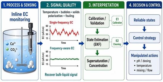
Graphical Abstract

1. Introduction

Precipitation reactions (carbonates, hydroxides, phosphates, sulfates, oxalates, and mixed salts) underpin impurity removal, selective recovery, scaling management, and product synthesis in mineral or chemical processing. In many flowsheets, product quality and operability depend on when nucleation starts, how supersaturation is relieved, and whether solids form in the intended reactor rather than in transfer lines or heat-exchange surfaces [1,2,3]. Despite this importance, inline monitoring remains challenging. Supersaturation is a thermodynamic construct inferred from composition, activity, and temperature, while practical process signals are indirect (EC, pH, density, turbidity, spectroscopy, image-based metrics). EC is especially appealing because probes are inexpensive, rugged, and easy to install, but it is only a scalar summary of a multidimensional ionic composition vector. The central challenge, therefore, is not whether EC responds to precipitation-related phenomena, but whether that response can be interpreted mechanistically and used consistently across changing compositions, temperatures, and multiphase conditions [4,5,6].
This manuscript is written as a practical review plus implementation blueprint for readers who may know EC instrumentation but are less familiar with model-based estimation/control. The main goal of this study is to show how EC can be used responsibly: literature is synthesized into a layered interpretive framework that clarifies what EC measures, when it works well, why it fails, and how measurement, calibration, estimation, and control can be connected in a chemical or mineral processing context [3,7,8,9]. A companion Supporting Document consolidates calibration-centric equations, modeling assumptions, estimator and controller formulations, computational model-oriented implementation logic, and demonstration results. To keep the discussion chemically concrete while preserving a broad scope, a Ca-carbonate/CaCO3 precipitation system is used throughout the manuscript as an illustrative case rather than as the sole or defining application domain [10,11]. This choice is deliberate because the coupling among conductivity, pH/speciation, supersaturation, and precipitation is unusually transparent in this system [3,7,8,12].

2. Precipitation and Crystallization Essentials

Only a limited set of precipitation and crystallization concepts is required for the EC-focused discussion in this review. Supersaturation is the driving force for nucleation and growth, but it is not measured directly in routine operation. Instead, it is inferred from temperature, composition, activity/speciation models, or indirect process signals such as EC, pH, density, turbidity, spectroscopy, and particle probes [1,2,8]. Induction time and nucleation onset are also important because a change in the slope or curvature of κ(t) may coincide with the transition from solution adjustment to solid formation, but such interpretation requires system-specific validation [12].
From an EC perspective, precipitation matters because it changes the population, mobility, and speciation of charge carriers. Conductivity may decrease when dominant ions are depleted, but pH shifts, background electrolytes, ion pairing, compensating feeds, or non-target ions can mask or distort this response [3,4]. This is why EC is best treated as an indirect, chemistry-dependent process feature rather than as a universal supersaturation indicator. In the Ca-carbonate/CaCO3 system, conductometric studies show that ion pairing and foreign salts can strongly affect early carbonate chemistry [10,11]. Nucleation studies further show that stable prenucleation clusters and particle-attachment pathways can occur on the nanoscale, which is relevant to nanomaterial-assisted precipitation and to the Special Issue theme [13,14,15].
The Ca-carbonate system is therefore used here as a chemically transparent case, not as the only target system. The same layered EC interpretation logic can also be relevant to Mg(OH)2 precipitation [16], BaSO4 precipitation with organic additives [17], freeze/eutectic crystallization of sulfate solutions [18], Li2CO3 precipitation from dilute Li-rich brines [19], and sequential mineral precipitation during seawater evaporation [20]. These examples illustrate that EC interpretation must be adapted to ionic strength, solids loading, pH/speciation chemistry, competing ions, and available validation data.

3. Electrical Conductivity Measurements in Aqueous Electrolytes

Electrical conductivity (κ, S m−1) quantifies the proportionality between current density and electric field, J = κ E. In a conductivity cell, κ is obtained from measured conductance G (=1/R) through κ = Kcell G, where Kcell is the cell constant. At the molecular level, conductivity arises from the concentration of charge carriers and their mobilities; in an idealized dilute system, κ may be expressed as a sum of ionic contributions κ = ∑(λi ci). Here, λi and ci represent molar ionic conductivity and ionic concentration of ion species i, respectively. The practical implication is central to this review: EC reports an aggregate transport property, not supersaturation itself [1,2,4]. For a single electrolyte in dilute solution, molar conductivity and limiting molar conductivity provide a transparent framework for interpreting curvature in κ-concentration relationships. In chemical or mineral-processing liquors, however, multi-ion composition, ion pairing, and activity effects make direct one-variable inversion fragile. Accordingly, the value of EC lies less in the existence of an electrical response itself rather than in whether the dominant charge carriers and their temperature- and composition-dependent behavior are sufficiently constrained for interpretation [4,5,6,21].
Temperature influences conductivity through viscosity, dielectric properties, and ion mobility. Routine process compensation often uses a linear correction around a reference temperature, but the correction coefficient is solution-specific and can vary with composition and concentration. This is why uncorrected—or over-generalized—temperature compensation can create false reaction signatures in cooling or otherwise non-isothermal crystallization. Temperature compensation should therefore be treated as a system-specific modeling choice rather than as a universal instrument setting [4,5,6]. In practical terms, EC becomes most informative when interpreted within a chemically constrained context; otherwise, it should be regarded as a sensitive but non-specific indicator that must be coupled with temperature, pH/speciation information, or model-based estimation. This is also why the same apparent conductivity change can correspond to quite different physicochemical events in carbonate, sulfate, hydroxide, phosphate, or mixed-liquor systems.

4. Literature Landscape and Critical Positioning of EC-Based Monitoring Within Crystallization PAT (Process Analytical Technology)

The literature relevant to EC-based precipitation and crystallization monitoring can be grouped into several connected areas: general crystallization monitoring, conductivity theory and calibration, direct EC/EIS (Electrochemical Impedance Spectroscopy) applications, nanoscale nucleation, mineral-processing precipitation systems, broader PAT instrumentation, and model-based estimation/control. This organization is useful because EC is neither a direct supersaturation sensor nor a complete crystallization analyzer. Instead, it is an indirect electrical feature whose value depends on whether the measured signal can be related to ionic composition, temperature, interfacial artifacts, and the target process state.
General crystallization-monitoring studies provide the basis for this interpretation. Zhang et al. reviewed solution concentration measurement methods in crystallization processes and positioned conductivity among broader concentration monitoring approaches [1]. Hlozný et al. demonstrated on-line supersaturation measurement during batch cooling crystallization of ammonium alum, showing that indirect concentration-related signals can track crystallization state in real time [2]. Löffelmann and Mersmann clarified why supersaturation is difficult to measure directly and why indirect signals must be interpreted through solubility, activity, and process-state information [8]. Söhnel and Mullin provided a classical method for determining precipitation induction periods, which remains relevant because changes in the EC slope or curvature can be meaningful only when linked to nucleation onset and induction-time behavior [12]. Yu et al. introduced the broader PAT concept for crystallization processes, emphasizing that sensors, modeling, chemometrics, and feedback control should be treated as connected elements rather than isolated tools [22]. Barrett et al. further reviewed PAT use in production batch crystallization and showed that process understanding typically requires multiple complementary measurements rather than a single probe response [23].
The electrochemical and calibration literature explains why EC interpretation must be handled carefully. Robinson and Stokes provide the electrolyte-solution foundation for understanding why conductivity depends on ionic concentration, mobility, ion pairing, and activity effects [4]. Wu et al. described primary standards for electrolytic conductivity, emphasizing that reliable EC measurement requires traceable calibration rather than only instrument readout [5]. Shreiner and Pratt provided standard reference materials for electrolytic conductivity, reinforcing the need for calibration continuity when conductivity is used for quantitative interpretation [6]. Schiefelbein et al. introduced a high-accuracy calibration-free technique for measuring liquid conductivity, which is important here because it shows how frequency-dependent electrical information can help recover a bulk conductive response rather than relying only on a nominal cell constant [9]. Yang et al. evaluated equivalent conductivities of silicate species in alkaline NaOH–Na2SiO3–H2O solutions, providing a reminder that multicomponent mineral-processing liquors require species-aware conductivity interpretation rather than simple one-solute calibration [21]. Ishai et al. reviewed electrode polarization in dielectric measurements, providing a basis for understanding why low-frequency artifacts, double-layer effects, and interfacial phenomena can distort conductivity-type measurements in electrolytes and suspensions [24]. Hallemans et al. further emphasized that EIS interpretation can be compromised when linearity, stability, or stationarity assumptions are violated, which is directly relevant to dynamic precipitation and crystallization processes [25].
Several prior studies directly connect EC, conductometry, or impedance to crystallization and precipitation monitoring. Hermanto et al. developed improved concentration control of crystallization using conductometry with reduced calibration effort, making it one of the most direct precedents for conductivity-derived concentration or supersaturation control [3]. Cao and Shah used in situ EC monitoring to gain mechanistic insight into zeolite crystallization, demonstrating that EC can reveal solution-to-solid transformation behavior in an aqueous crystallization process [26]. Hamdi and Tlili used conductometry to study the CaCO3 prenucleation stage and highlighted the role of neutral CaCO3 ion pairs in early carbonate chemistry [10]. Their later work showed that foreign salts influence the CaCO3 prenucleation stage, illustrating how background electrolytes can alter conductometric interpretation even within the same carbonate system [11]. Yuan et al. investigated Mg(OH)2 synthesis and crystallization kinetics, providing a non-carbonate example in which precipitation kinetics and ionic depletion must be interpreted in a system-specific way [16]. Das et al. linked kinetic characterization of precipitation reactions to reaction pathways, supporting the need to interpret conductivity transients in relation to precipitation mechanisms rather than as generic signal changes [27]. Mechi et al. examined barium sulfate precipitation under organic-additive effects, showing that additives can alter precipitation kinetics, morphology, and potentially conductivity-relevant trends in sulfate systems [17]. Amano and Louhi-Kultanen studied freeze and eutectic freeze crystallization in binary sulfate solutions, extending the relevance of the present discussion beyond conventional reactive precipitation to non-classical crystallization environments [18].
Recent EIS and frequency-dependent electrical studies further broaden the scope of EC-centered monitoring. Ghadipasha et al. used conductivity-based monitoring for non-isothermal antisolvent crystallization and showed that temperature-dependent concentration mapping is essential when crystallization occurs under changing thermal conditions [28]. Eder and Briesen extended scalar conductivity to EIS by fitting impedance spectra of sucrose suspensions with an equivalent circuit and relating resistance, capacitance, and constant-phase-element parameters to dissolved sucrose, crystalline sucrose, and salt content [29]. Their study is particularly relevant because it demonstrates both the promise and the limitations of EIS as a PAT tool: multiple electrical features can provide richer composition information than single-frequency EC, but dynamic operation can introduce scan-time and identifiability problems that require faster acquisition, better electrode design, or additional process constraints [29]. Rao et al. applied EIS to low-conductivity antisolvent crystallization and combined it with two-dimensional electrical resistance tomography, illustrating that electrical measurements can move beyond point conductivity toward spatially resolved process monitoring [30]. A subsequent study by Rao et al. showed that electrical tomography can visualize crystallization-induced heterogeneity that a single EC probe cannot resolve [31]. Zhao et al. used EIS to characterize crystallization processes and showed that impedance spectra change with crystallization progress in suspensions [32]. Zhao et al. later related crystal size to electrical impedance spectral features, supporting the view that frequency-dependent electrical measurements can contain both liquid-phase and suspension-structure information [33]. Nahvi and Hoyle presented wideband EIS sensing for industrial processes, which is relevant because acquisition time is a practical limitation when spectra are collected during rapidly changing crystallization conditions [34]. More recently, Zou et al. used machine learning to evaluate impedance spectra for glycine crystallization monitoring, showing that data-driven interpretation can help convert high-dimensional EIS features into crystallization-relevant information [35].
Nanoscale nucleation literature is also important for the Special Issue context. Gebauer et al. demonstrated stable prenucleation calcium carbonate clusters, providing a foundation for treating early CaCO3 formation as a nanoscale process rather than only a macroscopic precipitation event [13]. De Yoreo et al. reviewed crystallization by particle attachment in synthetic, biogenic, and geologic environments, showing that crystallization can proceed through clusters, amorphous particles, and nanoparticle attachment rather than only by classical ion-by-ion growth [14]. Gebauer and Cölfen reviewed prenucleation clusters and non-classical nucleation, further supporting the idea that EC changes during early precipitation may reflect changes in ionic speciation and nanoscale precursor populations rather than only bulk solute depletion [15]. These studies do not make EC a direct probe of nanoclusters; rather, they justify why EC should be interpreted together with speciation, pH, and complementary structural measurements when nucleation pathways are important.
The relevance of EC-based interpretation extends to mineral-processing and hydrometallurgical precipitation environments. Battaglia et al. investigated Li2CO3 precipitation from dilute Li-rich brines under varying carbonate dosage, ionic strength, temperature, and divalent-cation conditions, illustrating the type of chemically complex brine system in which EC must be interpreted together with pH, composition, and competing-ion effects [19]. Placencia-Gomez et al. applied spectral induced polarization to monitor induced calcite precipitation in sediments, demonstrating that frequency-dependent electrical responses can track mineral precipitation even in complex porous media [36]. Zhang et al. combined EIS with thermodynamic and kinetic analysis for gypsum precipitation in hypersaline solutions, making this study especially relevant to mineral-processing brines where high ionic strength and competing species complicate simple EC interpretation [37]. Rosenberg et al. examined mineral precipitation during seawater evaporation, including gypsum, celestine, and barite, illustrating that high-ionic-strength systems can involve sequential mineral formation and complex brine chemistry [20]. He et al. developed a high-precision calcium determination method for seawater, reinforcing the importance of orthogonal chemical validation when conductivity is used to infer carbonate precipitation behavior [38]. Chao et al. used in situ scattering and Raman spectroscopy to probe CaCO3 formation pathways, highlighting that nanoscale precursors and early clusters cannot be resolved by EC alone and require complementary structural probes [39].
Broader PAT and control studies clarify the position of EC relative to other monitoring tools. Advanced instrumental analyses such as Raman spectroscopy, ATR-FTIR ((Attenuated Total Reflectance-Fourier Transform Infrared), FBRM ((Focused Beam Reflectance Measurement), PVM (Particle Vision and Measurement), and image analysis can provide chemical, solid-form, particle-count, or morphology information that EC cannot directly resolve [22,23,39,40,41,42]. However, these techniques often require more complex instrumentation, optical access, chemometric calibration, or solids-handling precautions. Damour et al. developed a soft sensor for industrial sugar crystallization that estimated crystal mass, concentration, and purity online, illustrating how indirect signals can be converted into process-relevant latent variables [7]. A related model-based soft-sensor study by Damour et al. estimated crystal mass and solubility in industrial crystallization, supporting the use of observer-type inference when direct measurements are unavailable or incomplete [43]. Nagy and Braatz reviewed major advances in crystallization control and highlighted the importance of real-time concentration and particle-characterization measurements for feedback and model-based control [44]. Gao et al. reviewed PAT-based feedback control approaches in pharmaceutical crystallization and showed that feedback strategies depend strongly on the type and quality of online information available from solution and solid-state sensors [45]. Hermanto et al. showed that NMPC can be used for polymorphic transformation control, illustrating how model-based optimization can handle nonlinear crystallization dynamics and constraints when suitable state information is available [46]. De Moraes et al. applied modeling and predictive control to potassium sulfate cooling crystallization using dynamic image analysis, showing that non-EC sensors can also feed predictive controllers when they provide reliable state information [47]. Wang and Zhu developed a neural-network-based NMPC strategy for multiscale crystallization, indicating that data-driven surrogate models can be incorporated into advanced control architectures [48]. Xiouras et al. reviewed artificial intelligence and machine learning applications in crystallization and emphasized that data-driven methods are increasingly used to model, simulate, understand, and control complex crystallization systems [49]. Lima et al. further summarized recent developments in machine-learning-based modeling and advanced control of crystallization, highlighting the increasing role of data-driven models in state estimation and optimization [50].
Overall, these studies suggest that EC-based monitoring occupies a useful middle ground within crystallization PAT and mineral-processing precipitation monitoring. EC is less chemically specific than Raman or ATR-FTIR spectroscopy and less directly connected to particle attributes than FBRM, PVM, or image analysis, but it is simpler, cheaper, and often more robust for continuous aqueous operation. Frequency-aware conductivity extraction and EIS-informed processing can improve measurement integrity by separating bulk ionic response from polarization and interfacial artifacts, whereas soft sensors, observers, and predictive controllers can convert validated electrical features into process-relevant latent states. The novelty of the present review is therefore defined at the level of integration: the review connects measurement integrity, bulk-signal extraction, validation anchors, state estimation, and control readiness into a single deployment-oriented framework for precipitation and crystallization monitoring in mineral-processing environments.
The comparison in Table 1 clarifies the novelty and scope of the present review. Previous studies have demonstrated individual elements of the workflow, including EC/conductometric monitoring, EIS-based crystallization sensing, PAT instrumentation, soft-sensor estimation, and model-based control [3,7,23,24,25,29,30,31,32,33,34,35,43,44,45,46,47,48,49,50]. However, these elements have usually been discussed separately, either as sensor-specific methods, system-specific crystallization studies, or control-oriented case studies. The present review integrates these strands into a single deployment-oriented framework for precipitation and crystallization monitoring. Specifically, it links measurement integrity, frequency-aware conductivity extraction, orthogonal validation, state estimation, and control readiness in one layered structure. This framing clarifies when direct EC–T monitoring may be sufficient, when additional bulk-signal extraction or validation is required, and when EC-derived variables can reasonably support feedback control in mineral-processing precipitation and crystallization systems.

5. Measurement Layer: Deployment Modes and Acquisition

5.1. Inline, Online, Offline; Continuous vs. Intermittent

EC monitoring strategies can be classified by where the probe is located and how the sample is conditioned: inline immersion, on-line flow-through cells on slipstreams, side-stream filtered loops, and offline or intermittent grab sampling. These distinctions are not merely operational; they determine which part of the physicochemical reality is actually being sampled and how strongly the signal is exposed to solids, bubbles, fouling, and hydrodynamic artifacts. Representative in situ applications include solution-to-solid transformations such as zeolite crystallization and related aqueous systems [26,27]. Probe selection should be made jointly with installation design. Three practical configurations are especially common: (A) direct immersion in slurry (highest representativeness but highest artifact risk), (B) flow-through measurement on an unfiltered slipstream (better hydrodynamic control but continued exposure to solids), and (C) side-stream filtered monitoring (best bulk-liquid integrity but with possible lag and reduced sensitivity to slurry/interfacial effects). In this review, the A/B/C classification is used as a practical organizing device across precipitation systems, whereas the Ca-carbonate example should be read as one chemically explicit case situated within this broader deployment logic [1,3].

5.2. Calibration and Verification

Commercial EC probes do not eliminate the relevance of Kcell; they merely encapsulate it. Under clean, well-behaved conditions, routine calibration and temperature compensation may be sufficient. In precipitation service, however, solids, bubbles, scaling, corrosion, and geometry changes alter the effective current path. In practice, the relevant quantity is therefore not only the nominal manufacturer-specified cell constant, but also the effective cell constant and its drift under real process conditions [4,5,6,43]. Calibration and verification are thus not peripheral maintenance tasks but part of the core measurement design. Verification frequency should be chosen according to fouling propensity, process criticality, and acceptable uncertainty in inferred concentration or supersaturation. For long campaigns, cleaning and verification events should be treated as part of measurement design rather than as maintenance afterthoughts. Scheduled standard checks, clean-water/rinse checks, and cleaning-in-place (CIP) events can serve as traceability anchors that help distinguish sensor degradation from genuine process evolution [1,3]. In practice, two recurring anchors are especially useful: (E1) standard-solution checks that refresh the effective gain/cell constant and bound drift, and (E2) cleaning/CIP events that reset fouling-related offsets. These anchors become particularly important when conductivity is later translated into latent variables through soft-sensor or observer-based estimation.

6. Bulk Ionic Conductivity Extraction in Multiphase Media

Most EC meters use AC (Alternating Current) excitation and internally assume a mostly resistive response. Electrode polarization and capacitive effects are frequency dependent, and slurry suspensions may violate the assumptions embedded in simple instrument readouts. In this setting, the role of frequency-aware conductivity extraction is diagnostic as much as corrective: it may improve recovery of the bulk ionic contribution, but it can also reveal when no reliable bulk-conductivity feature is available under the prevailing multiphase conditions [9,24,25,34].
The term EIS-informed processing is used when equivalent-circuit fitting, spectral interpretation, or impedance-spectrum features are explicitly involved. Frequency-aware conductivity extraction uses multi-frequency information to identify a regime in which the measured impedance is dominated by bulk solution resistance. This should be viewed as a measurement-layer enhancement rather than as a universal replacement for conventional conductivity acquisition. Conductometric monitoring has also been applied to salt systems and precipitation processes (e.g., barium sulfate), where interfacial effects and additives modulate the apparent signal [3,17,28]. In many chemical or mineral-processing slurries, a clean bulk window may not always exist. Frequency-aware conductivity extraction should therefore be paired with diagnostics that flag when bulk extraction is unreliable. A carefully chosen high single frequency can sometimes approximate the bulk ionic conductivity, but this agreement is opportunistic and condition-dependent rather than guaranteed. At an architecture level, a comparison between frequency-aware conductivity extraction and fixed single-frequency readouts illustrates the practical point: the former is preferred because it separates measurement health from chemistry, while the latter can drift silently when polarization or interfacial dispersion changes [9].
In frequency-aware conductivity extraction, the measured impedance is written as Z(ω) = Z′(ω) + jZ″(ω), and the bulk ionic conductivity is estimated from the bulk resistance Rb through κbulk = Kcell/Rb. In single-frequency operation, however, Z′(ωs) may contain not only the bulk term Rb but also frequency-dependent polarization and interfacial contributions, e.g., Z′(ω) = Rb + ΔRpol(ω) + ΔRint(ω). Accordingly, κsingles) ≈ Kcell/Z′(ωs) can deviate from the true bulk conductivity, whereas a frequency-aware conductivity extraction estimate uses a bulk-dominated window Ωb to obtain estimated Řb (e.g., by averaging Rb values over Ωb) and hence κF-aware = Kcellb [9].
Figure 1 conceptually illustrates why bulk-signal extraction matters. Specifically, the hypothetical results comparing conductivity estimates were obtained using a frequency-aware conductivity extraction approach with conventional single-frequency readouts at 100 kHz and 1 kHz against the imposed “True” conductivity trajectory. The frequency-aware conductivity extraction estimate remains closely aligned with the true EC over the full run, indicating that using multi-frequency information to identify a bulk-dominated region effectively suppresses interfacial artifacts. In contrast, the single-frequency measurement at 1 kHz exhibits a pronounced deviation (a transient jump and subsequent relaxation between ~120 and 150 min), consistent with electrode polarization/dispersion effects contaminating the real-part impedance at that frequency and causing an apparent conductivity bias. The single-frequency trace at 100 kHz tracks the true EC much more closely in this particular scenario, suggesting that the chosen high frequency falls within a regime where polarization contributions are negligible and the measurement approximates the bulk solution resistance; however, this agreement is contingent on the operating conditions and should be regarded as opportunistic rather than guaranteed. Overall, the comparison highlights that frequency-aware conductivity extraction provides a more robust route to bulk ionic conductivity in the presence of time-varying interfacial effects, whereas single-frequency operation can be vulnerable to frequency-dependent polarization artifacts.

7. Mechanistic Interpretability Layer: From κ(t) to Latent States

One useful way to organize the literature and practice is to treat EC interpretation in real reactors through a unified measurement model that separates ionic conduction from gain, offset, slow drift/fouling, and slurry/bubble artifacts. This separation is valuable not because every application requires the same mathematical structure, but because it clarifies which part of the signal is plausibly chemical and which part may arise from measurement integrity or interfacial interference. Supporting Information provides a state-space form suitable for estimator integration.

7.1. Nonlinear Kalman Filtering as a Soft Sensor

Where chemistry is sufficiently constrained yet conductivity remains non-unique or drift-prone, observer-based estimation becomes attractive as a way to infer latent process variables from κ-T measurements. EKF (Extended Kalman Filter) and/or UKF (Unscented Kalman Filter)-type methods belong to this layer [52,53]. In the present manuscript, EKF examples are used as reference implementations because they are familiar, lightweight, and sufficient to demonstrate the architecture; in simpler systems, empirical or semi-empirical κ-T mappings may still be adequate [4,5,6,43]. In this framework, the filter estimates chemically meaningful latent variables (e.g., dissolved concentration or a supersaturation proxy) while simultaneously tracking nuisance parameters such as gain, offset, and slow drift. Innovation-based residual checks then provide a compact online plausibility test for measurement integrity. The estimator is therefore best viewed as an interpretive bridge between raw conductivity and chemically meaningful operating variables, rather than as an end in itself.

7.2. Linking Estimated States to an Exemplary Precipitation Interpretation

To make the abstract estimation logic concrete, a Ca-carbonate/CaCO3 precipitation system is used here. This choice does not imply that conductivity behaves identically across all precipitation systems; rather, the Ca-carbonate system is especially convenient because conductivity, pH/speciation, supersaturation, and precipitation kinetics are tightly coupled and chemically interpretable. Details of the carbonate-system closure used for this case are summarized in the Appendix A [10,11].
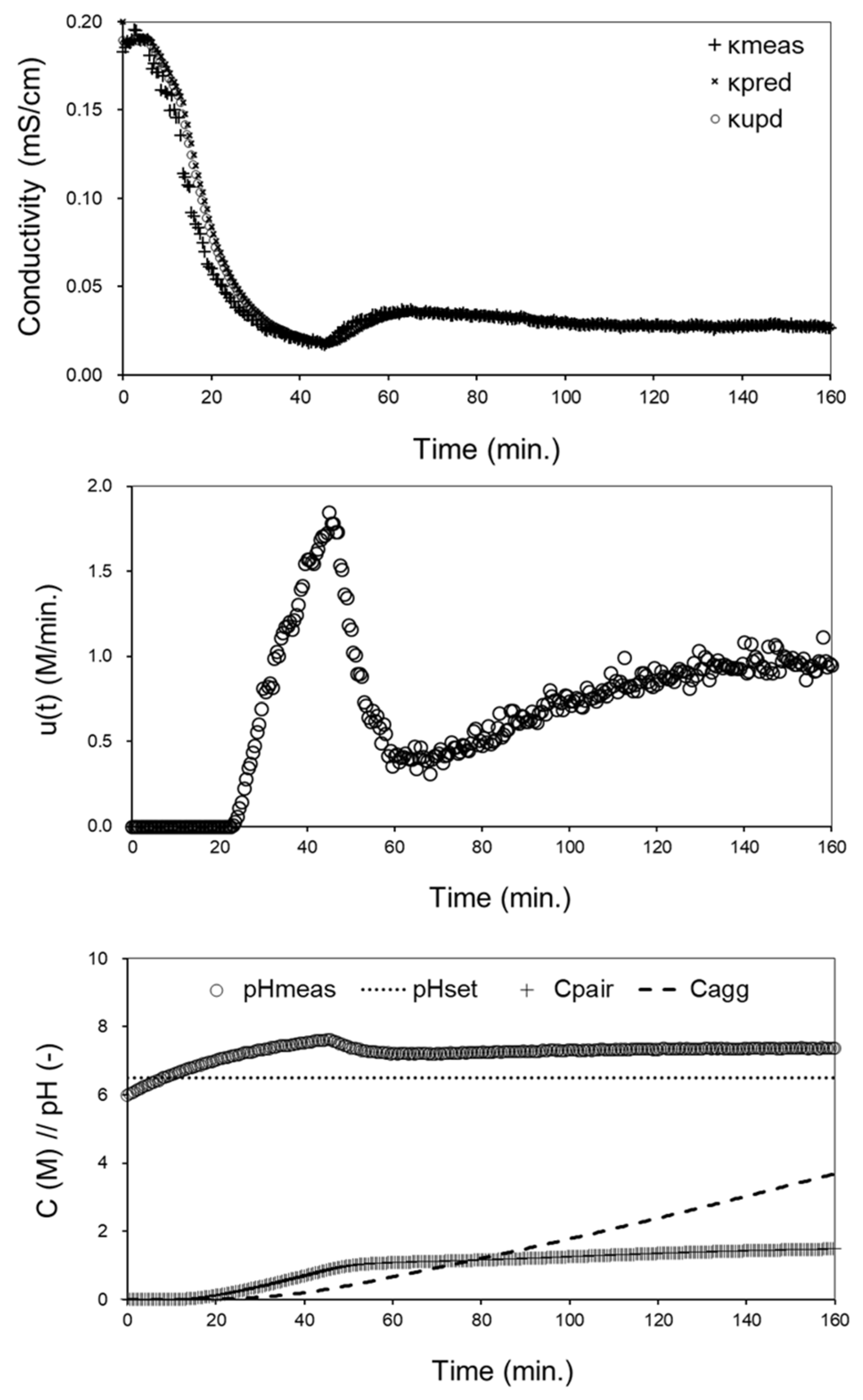
Figure 2 presents a conductometry-driven monitoring concept for this Ca-carbonate case. In this example, CO2 stripping raises pH, increases supersaturation, and promotes CaCO3 formation. The manipulated variable u(t) may therefore be interpreted as an effective stripping intensity, or a closely related actuation affecting pH and, in turn, supersaturation. The conductivity trajectories κmeas, κpred, and κupd illustrate how noisy measurements are reconciled with a reduced-order state model, while the accompanying pH trajectory and reduced prenucleation/aggregation proxies (e.g., Cpair and Cagg) provide a more chemically interpretable description of the evolving state. The top panel compares measured and EKF-reconstructed conductivity trajectories; the middle panel shows the manipulated actuation during the initial pH-ramp and subsequent maintenance period; and the bottom panel shows the associated pH evolution together with reduced ion-pairing and aggregation proxies. Taken together, these panels are intended as a pedagogical and architectural illustration of how conductivity-centered state estimation can be organized in one chemically transparent precipitation system, rather than as a claim of universal mechanistic representation.

8. Control Layer: Conductivity-Derived Targets and Feedback Operation

The control layer should be interpreted as a hierarchy of possible actions rather than as a requirement that every EC-monitored process must use advanced control. In the simplest case, EC is used for alarming, endpoint detection, or rule-based switching. In intermediate cases, EC-derived concentration or supersaturation proxies can support feedback control of a single manipulated variable, such as dosing rate, pH adjustment, antisolvent addition, cooling rate, gas-stripping intensity, or flow rate. In more demanding cases, MPC or NMPC becomes attractive because precipitation and crystallization processes are often nonlinear, constrained, and multivariable [3,44,45,46]. The key requirement is that the controlled variable should not be raw EC alone unless the EC–state relationship is well established. Instead, the control target should ideally be a validated EC-derived state, such as dissolved concentration, supersaturation proxy, or another chemically interpretable latent variable [7,35,43,45].

8.1. Conductivity-Derived Decision Variables and Setpoints

A conductivity-derived target may be constructed at several levels of sophistication. At the lowest level, the target can be a threshold or slope criterion, such as a change in dκ/dt indicating nucleation onset or deviation from an expected conductivity trajectory. This type of logic is suitable for event detection, endpoint detection, and operator decision support, especially when the process window is narrow and the chemistry is reproducible [1,2,12]. At a more quantitative level, κ–T calibration maps or semi-empirical conductivity–concentration models can convert EC and temperature into concentration estimates or supersaturation proxies, provided that composition and temperature effects are sufficiently constrained [3,28]. At the most model-based level, an observer or soft sensor can combine EC, temperature, pH, and validation anchors to estimate latent states while also tracking gain, offset, drift, or slurry/interfacial interference [7,35,43].
Within the Ca-carbonate framework, supersaturation is self-consuming: once CaCO3 formation begins, dissolved ionic precursors are depleted and the system tends to drift toward lower supersaturation. The control objective is therefore to maintain the process within a desired supersaturation or precipitation window without overcorrecting the chemistry. Depending on the process design, the manipulated input u(t) may represent Ca2+ or carbonate dosing, pH/alkalinity adjustment, CO2 stripping intensity, antiscalant or seed addition, temperature, mixing, or side-stream operation. In such cases, EC serves as the primary electrical measurement, while pH, temperature, and periodic chemical analyses provide validation and context [10,11,19,38].

8.2. Rule-Based Control, PID, MPC, and NMPC

Rule-based control is the most transparent form of conductivity-based operation. It can trigger actions when EC, dκ/dt, pH, or a conductivity-derived feature crosses a predefined threshold. This approach is simple and robust, but it is sensitive to drift, background electrolyte changes, and process-to-process variability. PID control can maintain a measured or estimated variable near a setpoint when the process is approximately single-input/single-output and the EC-derived state is sufficiently reliable. However, PID does not explicitly handle future constraint violations, multivariable interactions, or nonlinear supersaturation dynamics [44,45]. MPC and NMPC provide a more structured control layer by predicting the future evolution of the process over a finite horizon and selecting manipulated inputs subject to constraints. In precipitation and crystallization, these constraints may include actuator magnitude limits, move-rate limits, allowable pH or temperature ranges, maximum supersaturation, product-quality limits, or operational restrictions imposed by fouling and cleaning cycles [44,45,46,47,48]. NMPC is particularly relevant when the relationship among dosing, temperature, speciation, nucleation, growth, and conductivity is nonlinear. However, NMPC is not automatically superior; it requires a process-specific model or surrogate, reliable state estimates, uncertainty handling, and experimental validation [44,46,47,48,49,50].
In an EKF+NMPC architecture, the estimator and controller have distinct roles. The EKF or observer translates noisy EC–T data into a validated estimate of concentration, ionic conductivity, or supersaturation proxy. The NMPC layer then uses that estimate to compute feasible manipulated-input trajectories. Event anchors such as standard-solution checks, offline IC/ICP validation, pH/alkalinity checks, and cleaning/CIP events can be incorporated as parameter refreshes, pseudo-measurement updates, or covariance resets. Thus, EC-based control should be understood as a modular workflow: measurement first, validation second, estimation third, and feedback control fourth [3,7,35,43,45,46,47,48,49,50].
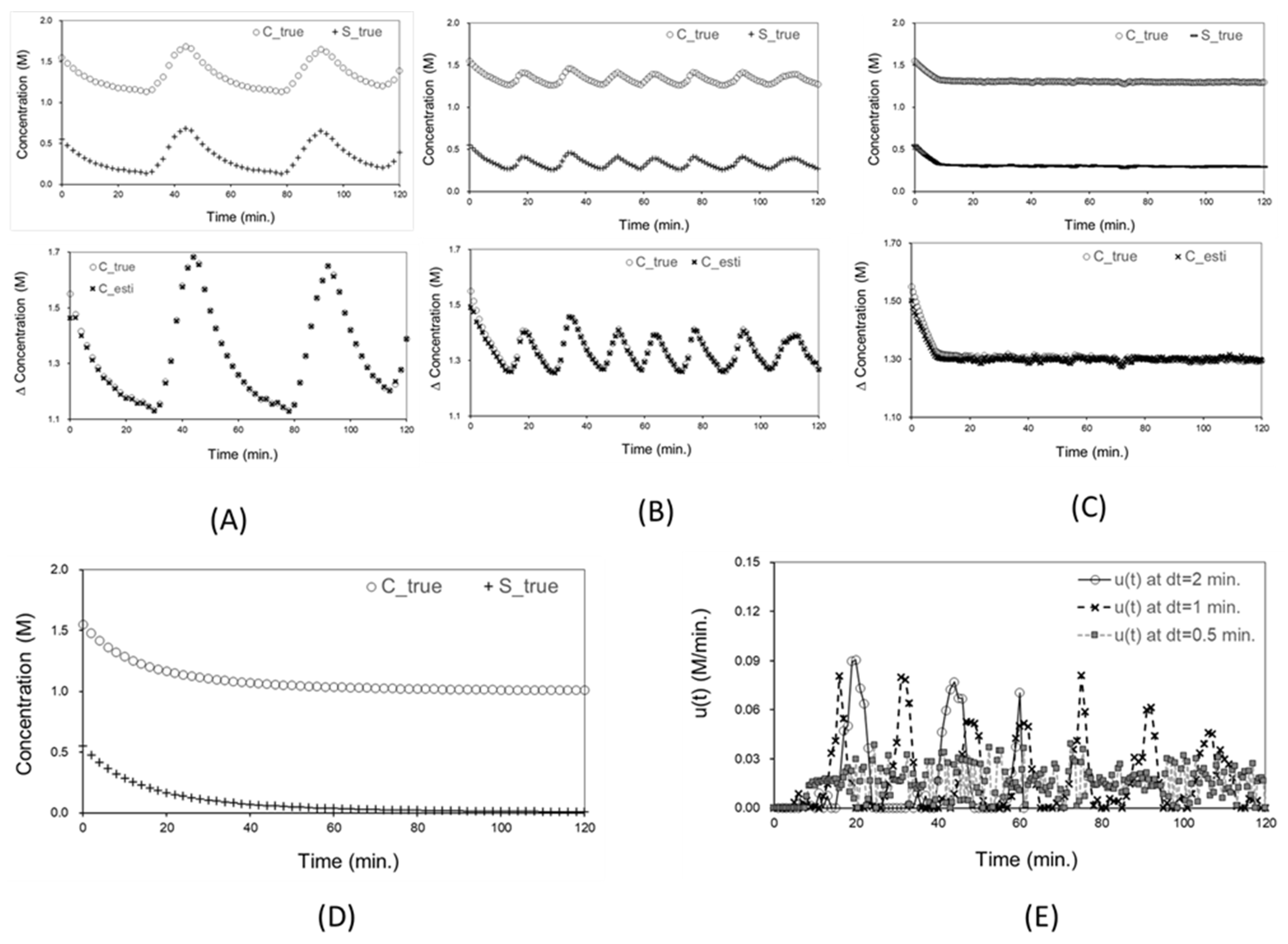
Figure 3 should therefore be read as an architecture demonstration rather than as proof of universal controller superiority. The comparison among update intervals illustrates a general control principle: shorter update intervals can permit smaller and more frequent corrective actions, whereas coarser updates can produce larger inter-sample excursions. The specific trajectories depend on the reduced-order model, tuning, and assumed noise structure. Accordingly, the practical contribution of the example is to show how conductivity-centered state estimation can feed a constrained control layer, not to prescribe a universal NMPC design for all precipitation or crystallization systems.

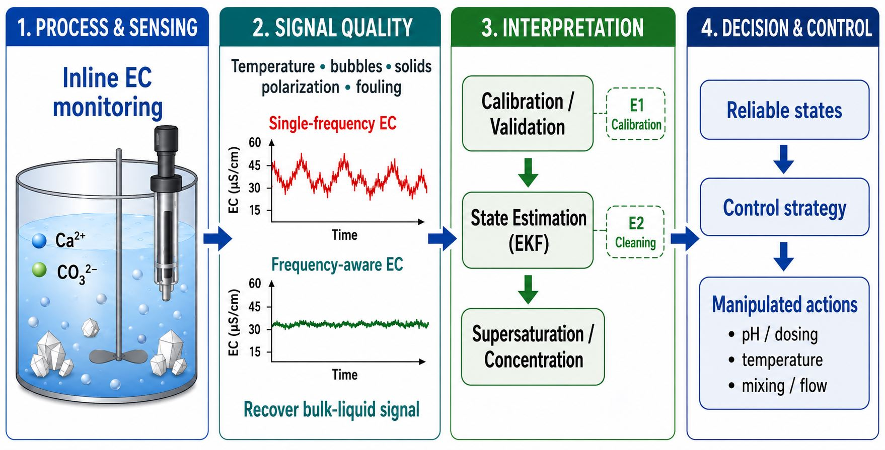
9. Practical Decision Framework

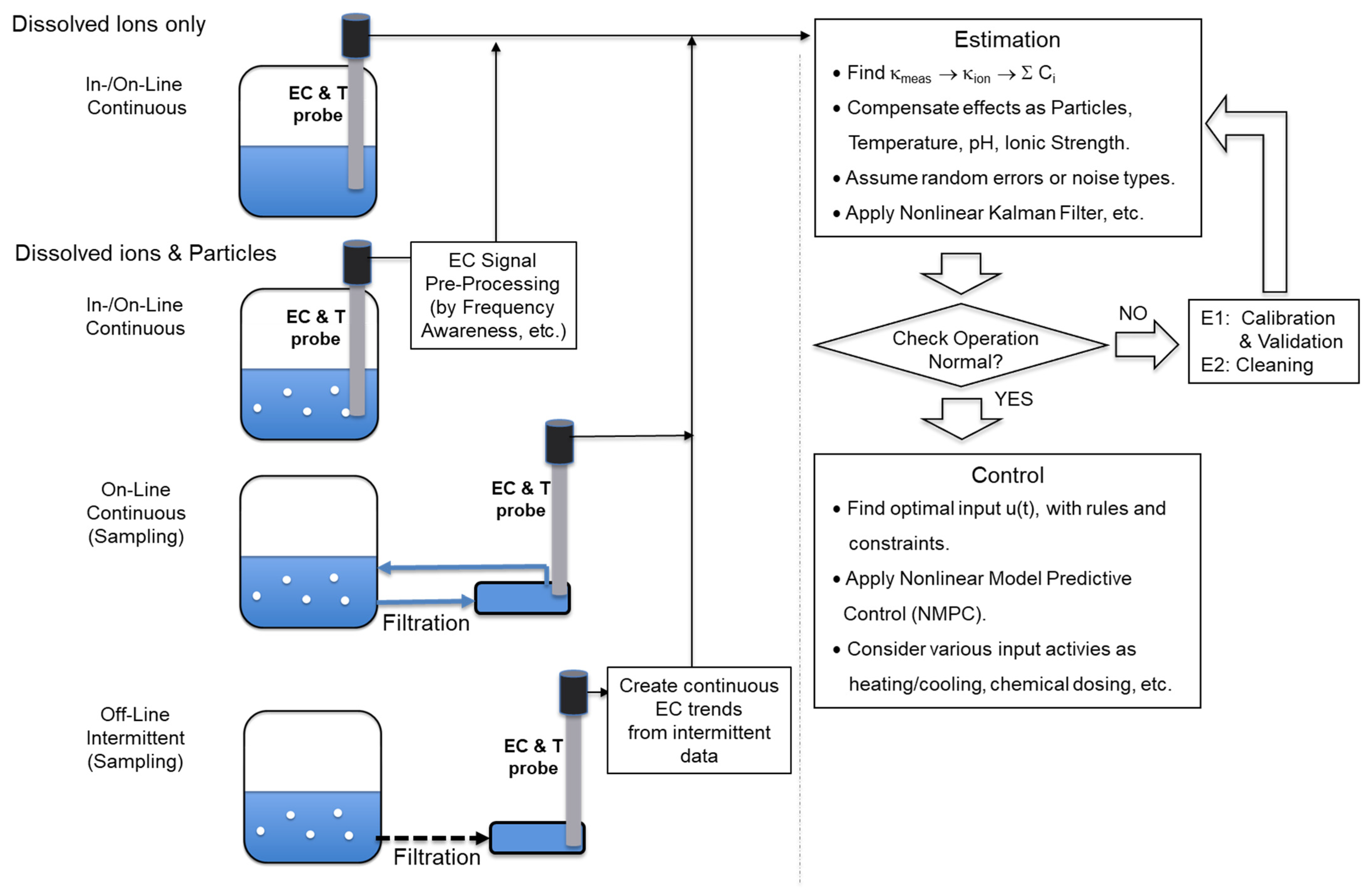
From a practical review perspective, the key question is not simply whether EC can be measured, but which conductivity signal is being measured, how trustworthy that signal is, and what level of physicochemical interpretation is justified. Figure 4 integrates deployment configuration, validation logic, state estimation, and control readiness into a single conceptual workflow. If the liquor is clear and the chemistry is relatively constrained, direct EC–T monitoring may be sufficient for useful process tracking. If solids, bubbles, fouling, or interfacial polarization obscure the bulk signal, deployment redesign and/or frequency-aware conductivity extraction become more important. If conductivity must be translated into dissolved concentration or supersaturation, calibration-assisted or observer-based estimation is justified. If the operating objective is sustained precipitation under process constraints, conductivity-derived targets can then support feedback control. Within this framework, the Ca-carbonate/CaCO3 example used throughout the review should be read as a concrete demonstration of the logic rather than as a restriction of applicability to carbonate precipitation alone.
Figure 4 also organizes conductivity-based monitoring according to where and how the probe is deployed, thereby linking inline, online, and offline acquisition modes to the level of signal conditioning and interpretation required. In single-phase liquids, a commercial inline probe or flow-through cell may provide adequate bulk-conductivity trends with minimal preprocessing. In contrast, bubble-rich or solids-containing systems often require additional measures such as side-stream conditioning, frequency-aware conductivity extraction analysis, or intermittent/off-line reconstruction to obtain an interpretable signal. Regardless of acquisition mode, the resulting EC–T data should pass through a validation layer—including drift checks, calibration anchors, plausibility tests, and, where appropriate, state estimation—before being used for concentration/supersaturation inference or control. At the architecture level, Figure 4 emphasizes a layered workflow: measurement first, validation second, estimation third, and control fourth. In this sequence, event anchors such as calibration checks and cleaning/CIP events help maintain traceability, while observer-based estimation and NMPC remain optional modules whose value increases with process complexity, nonlinearity, fouling risk, and the need for sustained operation. Table 2 and Table 3 complement this framework by summarizing typical use cases, applicability limits, common error sources, and practical mitigation strategies [1,3].

10. Research Gaps and Reporting Recommendations

A persistent gap is the lack of standardized, system-specific frameworks for interpreting κ in multicomponent chemical or mineral-processing liquors. Future studies should report the solution composition, temperature-control method, calibration protocol, probe type and material, installation mode, and excitation or frequency settings where applicable. They should also include at least one orthogonal validation signal, such as pH/alkalinity, IC/ICP analysis, turbidity, microscopy, XRD (X-Ray Diffraction), or mass balance [4,5,6]. A second gap is the limited integration of conductivity data with thermodynamic/speciation models and uncertainty analysis. Even when a full mobility model is unavailable, empirical κ–T–composition maps should be reported with the relevant operating window and uncertainty range. Such reporting would improve reproducibility and support industrial translation of EC-based monitoring [1,3]. For model-based implementations, authors should clearly distinguish the measurement, validation, estimation, and control layers. They should also state whether a reported algorithm is a process-specific optimized model or an educational/reference implementation [3,7,43]. This distinction is important because EKF, soft-sensor, and NMPC demonstrations can be useful for architecture design without being directly transferable to other precipitation systems.
Nanomaterials are relevant in two complementary ways. First, they can act as seeds, dopants, additives, or surface modifiers that influence nucleation barriers, growth pathways, aggregation, and polymorph selection. Second, they can be used as functional sensor coatings or engineered electrode interfaces that improve electrical transduction. Interdigitated electrodes, nanostructured sensing interfaces, and impedance/polarization approaches in complex media indicate a useful convergence between nanomaterial design and conductivity-based process monitoring [13,14,15,36,37,51].

11. Conclusions

Electrical conductivity is best viewed as an interpretable, low-cost electrical proxy whose value increases when paired with temperature measurement, calibration discipline, and chemically informed interpretation. It is highly effective for induction-time detection and trend monitoring, and it can support concentration or supersaturation inference in well-characterized systems. In complex chemical or mineral-processing liquors and slurries, conductivity-only interpretations of supersaturation are often unreliable. The strongest deployment pattern is therefore hybrid: robust sensor hardware and installation design, explicit calibration/verification workflow, bulk-signal extraction when needed, speciation- or model-aware interpretation, and soft-sensor or data-fusion support. To keep the framework concrete, a Ca-carbonate/CaCO3 system was used repeatedly as an illustrative case. That example should be read as a chemically transparent demonstration of the layered logic rather than as a restriction of applicability to carbonate precipitation alone. From mineral or chemical processing aspects, the practical contribution of this review is a deployment-oriented framework that links sensing, interpretation, validation, and control readiness.

Supplementary Materials

The following supporting document can be downloaded at: https://www.mdpi.com/article/10.3390/min16060658/s1, Supporting document: Calibration-Centric and Model-Based EC Monitoring for Aqueous Precipitation/Crystallization Companion to the manuscript: “Electrical Conductivity as an Inline Monitor for Aqueous Precipitation and Crystallization: Mechanistic Interpretability and a Model-Implementation Blueprint”.

Funding

This research was funded by 2030 Keimyung University Research Initiative program.

Data Availability Statement

Data are available from the corresponding author upon request.

Conflicts of Interest

The author declares no conflicts of interest.

Appendix A. Carbonate-System Theory for the Ca-Carbonate/CaCO3 Case

This appendix provides a compact theoretical foundation for (i) calculating supersaturation in Ca2+-carbonate systems, (ii) linking CaCO3 precipitation to ion depletion and pH change, and (iii) representing pH manipulation by CO2 stripping or related actuation. The formulations are intended as a mechanistically explicit back-end for process interpretation, not as a claim that all precipitation systems should be represented in the same way [10,11].

Appendix A.1. Carbonate Equilibria and Speciation with pH Dynamics

The aqueous inorganic carbon system comprises CO2(aq), H2CO3*, HCO3, and CO32− at temperature T. With H2CO3* denoting CO2(aq) + H2CO3, acid–base equilibria are written as:
H2CO3* ⇌ H+ + HCO3, K1(T) = a(H+) a(HCO3)/a(H2CO3*)
HCO3 ⇌ H+ + CO32−, K2(T) = a(H+) a(CO32−)/a(HCO3)
H2O ⇌ H+ + OH, Kw(T) = a(H+) a(OH)
Total dissolved inorganic carbon (DIC) is CT = [H2CO3*] + [HCO3] + [CO32−]. Given pH (e.g., −log10[H+]) and equilibrium constants, carbonate species fractions can be expressed through α-coefficients. A practical closure for pH uses total alkalinity AT, which is approximately conserved under CO2 stripping because stripping removes CO2 but does not directly add or remove strong acid/base. Neglecting minor contributors: AT ≈ [HCO3] + 2[CO32−] + [OH] − [H+]. When AT and CT are known from dosing, mass balances, or estimation, pH is obtained by solving the resulting one-dimensional alkalinity/charge-balance equation. For improved fidelity, Ca2+ complexation (e.g., CaHCO3+ and CaCO30) may be included when free-ion activities are needed for supersaturation calculations.

Appendix A.2. Supersaturation Toward CaCO3 Precipitation

Supersaturation can be expressed through the saturation ratio Ω = IAP/Ksp(T), where IAP = a(Ca2+)·a(CO32−). A convenient driving-force metric is S = ln(Ω), with Ω > 1 indicating supersaturation. Activities are related to concentrations by ai = γi[Ci], which can be used as a practical engineering approximation at moderate ionic strength. In high-salinity liquors, however, more advanced activity models may be required. At reactor scale, CaCO3 precipitation consumes Ca2+ and carbonate alkalinity and therefore changes both total calcium and dissolved inorganic carbon. For a well-mixed reactor with dosing and inlet/outlet flows, reduced balances can be written for total calcium and CT, while precipitation is represented by a kinetic surrogate such as Rprec = kprec·Max(Ω − 1, 0)n. The observed pH response should then be treated as a coupled outcome of carbonate equilibrium, alkalinity/DIC (Dissolved Inorganic Carbon) balances, precipitation, and gas-liquid mass transfer rather than as an independent driver.

Appendix A.3. CO2 Stripping as an Actuation Route

CO2 stripping is a useful actuation route because removing dissolved CO2 lowers H2CO3* and shifts carbonate equilibria toward HCO3 and CO32−, increasing pH at approximately constant alkalinity. In reduced form, d[CO2*]/dt may be written as a gas-transfer term driven by kLa and the deviation from equilibrium dissolved CO2 concentration. Within a mechanistically interpretable monitoring loop, one may (1) measure or estimate T and κ, (2) estimate composition states such as total calcium and CT or AT, (3) solve the pH closure if pH is not directly measured, (4) compute carbonate species and activities, (5) compute Ω and S, and (6) translate a supersaturation target into κset(T) and/or manipulated-input targets for control. Where full chemistry is not observable, these chemistry steps can be replaced by calibrated mappings; the main value of the appendix is to clarify what the Ca-carbonate example is meant to represent.

References

  1. Zhang, F.; Du, K.; Guo, L.; Huo, Y.; He, K.; Shan, B. Progress, problems, and potential of technology for measuring solution concentration in crystallization processes. Measurement 2022, 187, 110328. [Google Scholar] [CrossRef]
  2. Hlozný, L.; Sato, A.; Kubota, N. On-Line Measurement of Supersaturation during Batch Cooling Crystallization of Ammonium Alum. J. Chem. Eng. Jpn. 1992, 25, 604–606. [Google Scholar] [CrossRef][Green Version]
  3. Hermanto, M.W.; Phua, A.; Chow, P.S.; Tan, R.B.H. Improved C-control of crystallization with reduced calibration effort via conductometry. Chem. Eng. Sci. 2013, 97, 126–138. [Google Scholar] [CrossRef]
  4. Robinson, R.A.; Stokes, R.H. Electrolyte Solutions, 2nd ed.; Butterworths: London, UK, 1959; pp. 87–117. [Google Scholar]
  5. Wu, Y.C.; Knoch, W.F.; Pratt, K.W. Proposed new electrolytic conductivity primary standards for KCl solutions. J. Res. Natl. Inst. Stand. Technol. 1991, 96, 191–201. [Google Scholar] [CrossRef] [PubMed]
  6. Shreiner, R.H.; Pratt, K.W. Standard Reference Materials: Primary Standards and Standard Reference Materials for Electrolytic Conductivity; NIST Special Publication 260-142; National Institute of Standards and Technology: Gaithersburg, MD, USA, 2004; pp. 3–19.
  7. Damour, C.; Benne, M.; Grondin-Perez, B.; Chabriat, J.-P. Soft-sensor for industrial sugar crystallization: On-line mass of crystals, concentration and purity measurement. Control Eng. Pract. 2010, 18, 839–844. [Google Scholar]
  8. Löffelmann, M.; Mersmann, A. How to measure supersaturation? Chem. Eng. Sci. 2002, 57, 4301–4310. [Google Scholar] [CrossRef]
  9. Schiefelbein, S.L.; Fried, N.A.; Rhoads, K.G.; Sadoway, D.R. A high-accuracy, calibration-free technique for measuring the electrical conductivity of liquids. Rev. Sci. Instrum. 1998, 69, 3308–3313. [Google Scholar]
  10. Hamdi, R.; Tlili, M.M. Conductometric study of calcium carbonate prenucleation stage: Underlining the role of CaCO3o ion pairs. Cryst. Res. Technol. 2016, 51, 99–109. [Google Scholar]
  11. Hamdi, R.; Tlili, M.M. Influence of foreign salts on the CaCO3 prenucleation stage: Application of the conductometric method. CrystEngComm 2022, 24, 3256–3267. [Google Scholar]
  12. Söhnel, O.; Mullin, J.W. A method for the determination of precipitation induction periods. J. Cryst. Growth 1978, 44, 377–382. [Google Scholar] [CrossRef]
  13. Gebauer, D.; Völkel, A.; Cölfen, H. Stable prenucleation calcium carbonate clusters. Science 2008, 322, 1819–1822. [Google Scholar] [CrossRef] [PubMed]
  14. De Yoreo, J.J.; Gilbert, P.U.P.A.; Sommerdijk, N.A.J.M.; Penn, R.L.; Whitelam, S.; Joester, D.; Zhang, H.; Rimer, J.D.; Navrotsky, A.; Banfield, J.F.; et al. Crystallization by particle attachment in synthetic, biogenic, and geologic environments. Science 2015, 349, aaa6760. [Google Scholar] [CrossRef] [PubMed]
  15. Gebauer, D.; Cölfen, H. Prenucleation clusters and non-classical nucleation. Nano Today 2011, 6, 564–584. [Google Scholar] [CrossRef]
  16. Yuan, Q.; Lu, Z.; Zhang, P.; Luo, X.; Ren, X.; Golden, T.D. Study of the synthesis and crystallization kinetics of magnesium hydroxide. Mater. Chem. Phys. 2015, 162, 734–742. [Google Scholar] [CrossRef]
  17. Mechi, L.; Alshammri, K.S.K.; Alsukaibi, A.K.D.; Azaza, H.; Alimi, F.; Hedhili, F.; Moussaoui, Y. A study of the kinetics, structure, and morphology of the effect of organic additives on barium sulfate precipitation reactions in propan-1-ol–water and ethanol–water mixture solutions. Processes 2025, 13, 1471. [Google Scholar]
  18. Amano, B.; Louhi-Kultanen, M. Kinetics of freeze crystallization and eutectic freeze crystallization in binary aqueous solutions of Na2SO4, MgSO4, and CuSO4. Cryst. Growth Des. 2025, 25, 10320–10327. [Google Scholar]
  19. Battaglia, G.; Berkemeyer, L.; Cipollina, A.; Cortina, J.L.; Fernandez de Labastida, M.; Lopez Rodriguez, J.; Winter, D. Recovery of lithium carbonate from dilute Li-rich brine via homogenous and heterogeneous precipitation. Ind. Eng. Chem. Res. 2022, 61, 13589–13602. [Google Scholar] [CrossRef] [PubMed]
  20. Rosenberg, Y.O.; Sade, Z.; Ganor, J. The precipitation of gypsum, celestine, and barite and coprecipitation of radium during seawater evaporation. Geochim. Cosmochim. Acta 2018, 233, 50–65. [Google Scholar] [CrossRef]
  21. Yang, K.; Ye, G.; De Schutter, G. Study and evaluation of equivalent conductivities of [SiO(OH)3] and [SiO2(OH)2]2− in NaOH-Na2SiO3-H2O Solutions at 277.85 K to 308.45 K. Materials 2025, 18, 2996. [Google Scholar] [PubMed]
  22. Yu, L.X.; Lionberger, R.A.; Raw, A.S.; D’Costa, R.; Wu, H.; Hussain, A.S. Applications of process analytical technology to crystallization processes. Adv. Drug Deliv. Rev. 2004, 56, 349–369. [Google Scholar] [CrossRef] [PubMed]
  23. Barrett, P.; Smith, B.; Worlitschek, J.; Bracken, V.; O’Sullivan, B.; O’Grady, D. A review of the use of process analytical technology for the understanding and optimization of production batch crystallization processes. Org. Process Res. Dev. 2005, 9, 348–355. [Google Scholar] [CrossRef]
  24. Ishai, P.B.; Talary, M.S.; Caduff, A.; Levy, E.; Feldman, Y. Electrode polarization in dielectric measurements: A review. Meas. Sci. Technol. 2013, 24, 102001. [Google Scholar] [CrossRef]
  25. Hallemans, N.; Howey, D.; Battistel, A.; Saniee, N.F.; Scarpioni, F.; Wouters, B.; La Mantia, F.; Hubin, A.; Widanage, W.D.; Lataire, J. Electrochemical impedance spectroscopy beyond linearity and stationarity—A critical review. Electrochim. Acta 2023, 466, 142939. [Google Scholar] [CrossRef]
  26. Cao, G.; Shah, M.J. In situ monitoring of zeolite crystallization by electrical conductivity measurement: New insight into zeolite crystallization mechanism. Microporous Mesoporous Mater. 2007, 101, 19–23. [Google Scholar] [CrossRef]
  27. Das, N.P.; Zahorán, R.; Janovák, L.; Deák, Á.; Tóth, Á.; Horváth, D.; Schuszter, G. Kinetic characterization of precipitation reactions: Possible link between a phenomenological equation and reaction pathway. Cryst. Growth Des. 2020, 20, 7392–7398. [Google Scholar] [CrossRef]
  28. Ghadipasha, N.; Baratti, R.; Tronci, S.; Romagnoli, J.A. A deterministic formulation and on-line monitoring technique for the measurement of salt concentration in non-isothermal antisolvent crystallization processes. Chem. Eng. Trans. 2015, 43, 1375–1380. [Google Scholar]
  29. Eder, C.; Briesen, H. Impedance spectroscopy as a process analytical technology (PAT) tool for online monitoring of sucrose crystallization. Food Control 2019, 101, 251–260. [Google Scholar] [CrossRef]
  30. Rao, G.; Aghajanian, S.; Koiranen, T.; Wajman, R.; Jackowska-Strumillo, L. Process monitoring of antisolvent based crystallization in low conductivity solutions using electrical impedance spectroscopy and 2-D electrical resistance tomography. Appl. Sci. 2020, 10, 3903. [Google Scholar] [CrossRef]
  31. Rao, G.; Aghajanian, S.; Zhang, Y.; Jackowska-Strumiłło, L.; Koiranen, T.; Fjeld, M. Monitoring and visualization of crystallization processes using electrical resistance tomography: CaCO3 and sucrose crystallization case studies. Sensors 2022, 22, 4431. [Google Scholar] [CrossRef] [PubMed]
  32. Zhao, Y.; Wang, M.; Hammond, R.B. Characterization of crystallisation processes with electrical impedance spectroscopy. Nucl. Eng. Des. 2011, 241, 1938–1944. [Google Scholar] [CrossRef]
  33. Zhao, Y.; Yao, J.; Wang, M. On-line monitoring of the crystallization process: Relationship between crystal size and electrical impedance spectra. Meas. Sci. Technol. 2016, 27, 074007. [Google Scholar] [CrossRef]
  34. Nahvi, M.; Hoyle, B.S. Electrical impedance spectroscopy sensing for industrial processes. IEEE Sens. J. 2009, 9, 1808–1816. [Google Scholar] [CrossRef]
  35. Zou, J.J.; Eder, C.; Briesen, H. A machine learning approach to evaluate impedance spectra for glycine crystallization monitoring. Ind. Eng. Chem. Res. 2026, 65, 8056–8068. [Google Scholar] [CrossRef]
  36. Placencia-Gomez, E.; Robinson, J.; Slater, L.; Qafoku, N.P. Spectral induced polarization monitoring of induced calcite precipitation in subsurface sediments. Geophys. J. Int. 2023, 232, 57–69. [Google Scholar]
  37. Zhang, Z.; Pawar, R.D.; Vidic, R.D. Study of thermodynamic models and crystallization kinetics for gypsum precipitation in hypersaline solutions with electrochemical impedance spectroscopy (EIS). Desalination 2025, 613, 119025. [Google Scholar] [CrossRef]
  38. He, H.; Li, Y.; Wang, S.; Ma, Q.; Pan, Y. A high precision method for calcium determination in seawater using ion chromatography. Front. Mar. Sci. 2020, 7, 231. [Google Scholar] [CrossRef]
  39. Chao, Y.; Horner, O.; Vallée, P.; Meneau, F.; Alos-Ramos, O.; Hui, F.; Turmine, M.; Perrot, H.; Lédion, J. In situ probing calcium carbonate formation by combining fast controlled precipitation method and small-angle X-ray scattering. Langmuir 2014, 30, 3303–3309. [Google Scholar] [PubMed]
  40. O’Sullivan, B.; Glennon, B. Application of in situ FBRM and ATR-FTIR to the monitoring of the polymorphic transformation of D-mannitol. Org. Process Res. Dev. 2005, 9, 884–889. [Google Scholar] [CrossRef]
  41. Liu, F.; Bagi, S.D.; Su, Q.; Chakrabarti, R.; Barral, R.; Gamekkanda, J.C.; Hu, C.; Mascia, S. Targeting particle size specification in pharmaceutical crystallization: A review on recent process design and development strategies and particle size measurements. Org. Process Res. Dev. 2022, 26, 3190–3203. [Google Scholar] [CrossRef]
  42. Orehek, J.; Teslić, D.; Likozar, B. Continuous crystallization processes in pharmaceutical manufacturing: A review. Org. Process Res. Dev. 2021, 25, 16–42. [Google Scholar]
  43. Damour, C.; Benne, M.; Grondin-Perez, B.; Chabriat, J.-P. Model based soft-sensor for industrial crystallization: On-line mass of crystals and solubility measurement. Int. J. Biol. Life Agric. Sci. 2009, 3, 275–282. [Google Scholar]
  44. Nagy, Z.K.; Braatz, R.D. Advances and new directions in crystallization control. Annu. Rev. Chem. Biomol. Eng. 2012, 3, 55–75. [Google Scholar] [CrossRef] [PubMed]
  45. Gao, Y.; Zhang, T.; Ma, Y.; Xue, F.; Gao, Z.; Hou, B.; Gong, J. Application of PAT-based feedback control approaches in pharmaceutical crystallization. Crystals 2021, 11, 221. [Google Scholar] [CrossRef]
  46. Hermanto, M.W.; Chiu, M.-S.; Braatz, R.D. Nonlinear model predictive control for polymorphic transformation of L-glutamic acid crystals. AIChE J. 2009, 55, 2631–2645. [Google Scholar]
  47. de Moraes, M.G.F.; Lima, F.A.R.D.; da Cunha Lage, P.L.; de Souza, M.B., Jr.; Barreto, A.G., Jr.; Secchi, A.R. Modeling and predictive control of cooling crystallization of potassium sulfate by dynamic image analysis: Exploring phenomenological and machine learning approaches. Ind. Eng. Chem. Res. 2023, 62, 9515–9532. [Google Scholar] [CrossRef]
  48. Wang, L.; Zhu, Y. Neural-network-based nonlinear model predictive control of multiscale crystallization process. Processes 2022, 10, 2374. [Google Scholar]
  49. Xiouras, C.; Cameli, F.; Quilló, G.L.; Kavousanakis, M.E.; Vlachos, D.G.; Stefanidis, G.D. Applications of artificial intelligence and machine learning algorithms to crystallization. Chem. Rev. 2022, 122, 13006–13042. [Google Scholar] [CrossRef] [PubMed]
  50. Lima, F.A.R.D.; de Moraes, M.G.F.; Barreto, A.G., Jr.; Secchi, A.R.; Grover, M.A.; de Souza, M.B., Jr. Applications of machine learning for modeling and advanced control of crystallization processes: Developments and perspectives. Digit. Chem. Eng. 2025, 14, 100208. [Google Scholar]
  51. Tong, J.; Doumbia, A.; Turner, M.L.; Casiraghi, C. Real-time monitoring of crystallization from solution by using an interdigitated array electrode sensor. Nanoscale Horiz. 2021, 6, 468–473. [Google Scholar] [CrossRef] [PubMed]
  52. Simon, D. Chapter 14: The unscented Kalman filter. In Optimal State Estimation Kalman, H, and Nonlinear Approaches; John Wiley & Sons, Inc.: Hoboken, NJ, USA, 2006; pp. 433–459. [Google Scholar]
  53. de Vallière, P.; Agarwal, M.; Bonvin, D. Experimental estimation of concentrations from reactor temperature measurement. In Proceedings of the 2nd International IFAC Symposium on Adaptive Control of Chemical Processes 1988 (ADCHEM ‘88), Lyngby, Denmark, 17–19 August 1988; pp. 183–188. [Google Scholar]
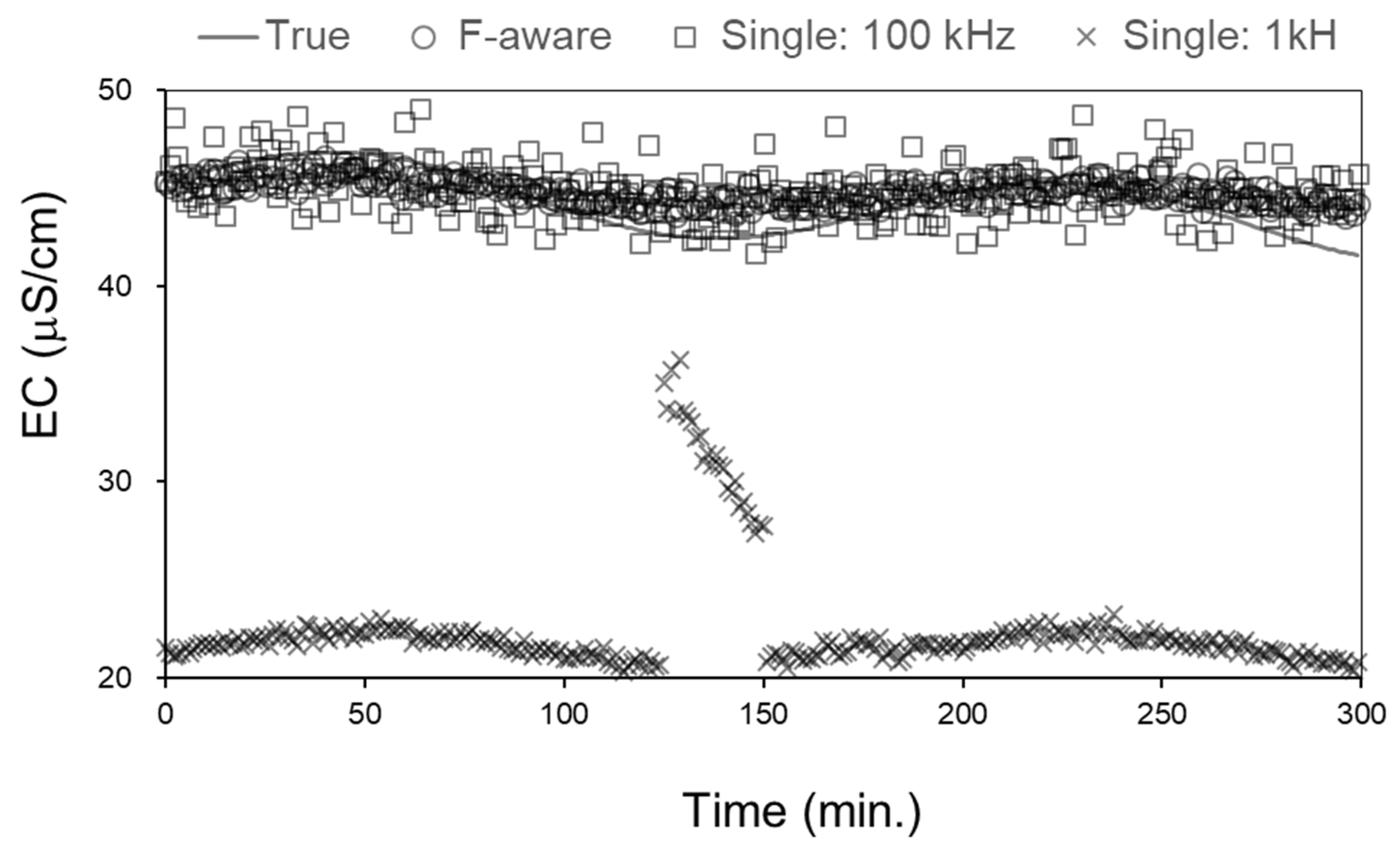
Figure 1. Architecture-level comparison of frequency-aware conductivity extraction (F-aware: hollow circle symbols) and fixed single-frequency readouts at 100 kHz (Single: 100 kHz: hollow square symbols) and 1 kHz (Single: 1 kHz: “×” symbols), with true EC (solid line).
Minerals 16 00658 g001
Figure 2. Conductometry-driven monitoring and control concept for a Ca–carbonate system, showing measured (κmeas), predicted (κpred), and updated (κupd) conductivity trajectories (top plot), manipulated actuation (middle plot), and pH evolution together with reduced prenucleation (Cpair) or aggregation (Cagg) proxies (bottom plot). Here, pHmeas and pHset denote the measured pH and target pH values, respectively.
Minerals 16 00658 g002
Figure 3. Architecture demonstration of closed-loop supersaturation control in the Ca-carbonate case, comparing different sampling intervals (Δt = 2, 1, and 0.5 min for (A), (B), and (C), respectively) and an open-loop reference (D) together with manipulated actuation in order to maintain supersaturation within a constant range (E).
Minerals 16 00658 g003
Figure 4. Practical decision framework linking deployment configuration, validation anchors, state estimation, and conductivity-derived control readiness for precipitation or crystallization systems.
Minerals 16 00658 g004
Table 1. Comparison of common process variables and instrumentation for precipitation/crystallization monitoring.
Measured Variable/InstrumentationPrimary Information ObtainedTypical Performance and Deployment CharacteristicsMain StrengthsMain LimitationsRole Relative to EC-Based MonitoringKey Refs
Electrical conductivity (EC)/conductometryAggregate ionic transport property reflecting charge-carrier concentration and mobilityFast response, low cost, simple inline deployment; good for clear aqueous liquors; moderate robustness in slurries if cleaning and validation are adequateRugged, inexpensive, easy to install, sensitive to ionic depletion/speciation changes, useful for induction-time and reaction-progress trackingNon-specific; affected by temperature, background electrolytes, ion pairing, bubbles, solids, fouling, and electrode polarization; does not directly measure supersaturationCore signal of this review; useful when interpreted with temperature, calibration, speciation, and validation rather than as a direct supersaturation sensor[3,4,5,6,10,11,21,26,51]
Frequency-aware EC/
EIS-informed electrical measurement
Frequency-dependent impedance response; bulk resistance, interfacial polarization, dielectric/suspension featuresResponse depends on frequency scan or discrete-frequency acquisition; medium cost/complexity; inline possible but sensitive to scan time and stationarityCan separate bulk ionic response from electrode/interface artefacts; provides richer electrical features than single-frequency EC; useful under polarization or slurry effectsRequires multi-frequency acquisition, equivalent-circuit or feature extraction, and diagnostics; dynamic processes can violate stationarity assumptions; electrode design is importantExtends EC from scalar readout to measurement-integrity analysis and bulk-signal extraction[9,24,25,29,30,31,35,51]
pH/alkalinityAcid–base state, carbonate/hydroxide/phosphate speciation, neutralization progressFast response, low cost, widely used inline; good for carbonate and hydroxide systems; maintenance required in scaling liquorsDirectly relevant to pH-driven precipitation, CO2 stripping, alkalinity control, and hydroxide/carbonate precipitationDoes not directly quantify dissolved precursor concentration, solids formation, or supersaturation; electrode drift and fouling can occurEssential companion variable for EC in systems where ionic depletion is coupled with acid–base speciation[10,11,19]
TemperatureThermal driving force, solubility shift, ion mobility, compensation variableVery fast, low cost, robust inline measurement; required for most concentration and solubility calculationsEssential for EC correction, solubility/supersaturation calculation, and non-isothermal crystallization interpretationTemperature alone is not a composition or precipitation measurement; thermal gradients can cause local misinterpretationRequired auxiliary variable for EC calibration, conductivity compensation, and state estimation[3,4,5,6,22,28]
Density/refractive index/microwave or acoustic concentration proxiesBulk concentration, total solute content, density-related process stateFast to moderate response; generally medium cost; inline or online implementation possible depending on probe typeUseful for concentration tracking in crystallization liquors; can provide information not captured by EC when nonionic solutes dominateCross-sensitive to temperature, purity, bubbles, and suspended solids; usually limited chemical specificityComplementary concentration proxy when EC is weakly sensitive or dominated by background ions[1,22,23]
Turbidity/optical transmissionOnset of particle formation, cloud point, qualitative solid formationFast and relatively low cost; inline possible in transparent or moderately turbid systems; performance declines at high solids loadingSensitive to nucleation/solid appearance; useful for induction-time detectionNon-specific; affected by bubbles, particle size, color, optical fouling, and high suspension opacity; weak for dissolved-state inferenceComplements EC by detecting optical solid formation when EC changes are ambiguous[12,22,23,41]
Raman spectroscopyMolecular identity, solute concentration, polymorphic form, desupersaturation behaviorMedium-to-fast response depending on acquisition; high cost; inline possible with optical probe and chemometric calibrationChemically selective; can distinguish polymorphs and provide concentration/solid-form informationRequires optical access, calibration models, fouling control, and adequate signal quality; fluorescence or opacity may interfereProvides chemical specificity that EC lacks; useful as validation or complementary PAT for concentration and solid-form information[22,23,39,40]
ATR-FTIR/
NIR spectroscopy
Liquid-phase concentration, functional-group information, reaction or solute trackingMedium-to-fast response; medium-to-high cost; inline/online possible with probe or flow cellStrong for solution concentration monitoring and chemometric calibrationOptical fouling, contact/path-length issues, calibration transfer, and reduced solid-form specificity compared with RamanProvides chemically selective liquid-phase information for EC calibration, soft-sensor development, or validation[22,23,40]
FBRM/PVM/
In-situ imaging
Chord-length distribution, particle count, qualitative morphology, particle-size evolutionFast to moderate response; medium-to-high cost; inline slurry deployment possible if optics remain cleanDirectly probes solid-phase evolution, nucleation, growth, agglomeration, breakage, and morphologyDoes not directly measure dissolved ionic state or supersaturation; chord length is not identical to true PSD; fouling and dense suspensions complicate interpretationSupplies particle information unavailable from EC; best combined with EC when liquid-phase and solid-phase dynamics both matter[23,40,41,42,47]
ERT/SIP/electrical tomography or geoelectrical monitoringSpatially resolved or frequency-dependent electrical response in vessels, porous media, or heterogeneous systemsModerate response depending on inversion and acquisition; higher instrumentation/modeling complexity than EC; useful in opaque systemsCan reveal spatial heterogeneity and precipitation-induced electrical changes beyond a single probeLower chemical specificity; requires inverse modeling and geometry-dependent interpretationExtends EC/EIS concepts to spatially heterogeneous or porous-media mineral precipitation systems[30,31,36]
Offline IC/ICP, titration, XRD, microscopy, or mass balanceIon concentrations, elemental composition, phase identity, morphology, and independent mass/charge balanceSlow or intermittent; laboratory-based; high analytical specificity; not a real-time control signalProvides ground truth for calibration, validation, and mechanism confirmationDiscontinuous, labor-intensive, and delayed; cannot directly support fast feedback unless used for periodic updatingEssential validation layer for EC interpretation in chemically complex liquors and brines[19,20,38]
Soft sensors/
observer-based estimation
Latent variables such as dissolved concentration, crystal mass, supersaturation proxy, drift/interference statesReal-time once implemented; computational cost usually modest; performance depends on input-signal quality and model validityConverts indirect signals into process-relevant states; can combine EC, temperature, pH, PAT, and offline dataRequires model structure, calibration, uncertainty handling, and validation; model mismatch can bias estimatesKey bridge between raw EC and control-relevant variables in the present framework[7,35,43,44,45,47,48,49,50]
PID/MPC/
NMPC feedback control
Manipulated-input policy for maintaining supersaturation, concentration, temperature, or product-quality targetsReal-time computational layer; performance depends on sensor reliability, model quality, constraints, and tuningHandles feedback, constraints, multivariable dynamics, and predictive optimizationRequires reliable state information and process-specific validation; poorFinal layer in which EC becomes useful only after validation and translation into interpretable target variables[3,44,45,46,47,48,49,50]
Table 2. Typical use cases for EC monitoring in aqueous precipitation and recommended analysis strategy.
CasesEC Measurement
Objectives
Primary OutputsRecommended PointsKey Refs
Induction time
detection
Fast precipitation with clear solute depletion signatureinduction time vs. Supersaturation (S) levels;
additive/seed effects
High-rate sampling; controlled mixing;
temperature logging
[1,12]
Reaction
progress
Simple ionic systems; stable composition; low–moderate ionic strengthSolute concentration vs. time;
kinetic curves
Calibration EC–C–T; speciation model if needed[5,8,9,12,16,26,27]
Supersaturation
inference
Known composition + validated solubility modelEstimated S(t);
control trajectory
Temperature compensation; electrolyte/activity model[2,6,8]
Harsh process
liquor monitoring
As a proxy feature rather than primary measurementChange-point;
anomaly detection
Sensor fusion + soft sensor/observer[2,3,7,43]
Table 3. Common error sources in EC monitoring and practical mitigation.
Error SourceMechanismMitigationKey Refs
Temperature driftMobility increases with T;
EC varies even at constant concentration
Inline temperature probe;
automatic temperature compensation;
[4,5,6,28]
Composition or impuritiesNon-target ions dominate conductivity;
EC–supersaturation mapping breaks down
Track key ions with other instrumental analyses (IC/ICP);
electrolyte model;
soft sensor;
periodic recalibration
[3,7,43]
Electrode polarizationLow-frequency artifacts;
contact impedance
Four-electrode cell;
AC measurement;
multi-frequency diagnostics
[9,24,25,34]
Fouling/scalingDeposits alter cell constant;
drift
Inductive sensors; cleaning/CIP; anti-fouling coatings;
health checks
[4,5,6,9]
Bubbles/solidsPathway disruption;
noise
Flow-through cell design;
degassing;
signal filtering;
combine with e.g., turbidity
[24,25,30,31,34]
Disclaimer/Publisher’s Note: The statements, opinions and data contained in all publications are solely those of the individual author(s) and contributor(s) and not of MDPI and/or the editor(s). MDPI and/or the editor(s) disclaim responsibility for any injury to people or property resulting from any ideas, methods, instructions or products referred to in the content.