Article

A Robust GDF-ML Framework for Dynamic Grade Modeling: Adaptive Resource Estimation in Complex Porphyry Systems


MCC Tongsin Resources Ltd., Beijing 100028, China
Minerals 2026, 16(6), 573; https://doi.org/10.3390/min16060573
Submission received: 13 March 2026 / Revised: 21 May 2026 / Accepted: 24 May 2026 / Published: 27 May 2026

Abstract

Accurate grade estimation in heterogeneous porphyry copper deposits is frequently constrained by spatial non-stationarity and the excessive smoothing inherent in traditional geostatistical methods. This study introduces the Geological Distance Field-Machine Learning (GDF-ML) framework, which transforms raw spatial coordinates into a geological coordinate system defined by the structural architecture. By mapping grade distribution within this geologically informed space, the framework enables machine learning models to discern non-linear mineralizing patterns that are typically obscured in traditional Euclidean 3D space. Functioning as an expert-constrained regression architecture rather than a purely data-driven interpolator, the framework estimates grade distributions conditional upon established metallogenic controls. In this context, the achieved spatial separation cross-validation R2 of 0.851 quantifies the proportion of grade variance structurally explainable by the geological architecture, highlighting the workflow’s capacity to distinguish continuous structural trends from localized random variability. Industrial reconciliation against high-density production data confirms this performance, demonstrating an average grade bias of only 0.79%, compared to 9.68% achieved by Ordinary Kriging. Furthermore, SHAP analysis verifies that these predictions are systematically driven by the non-linear relationship between structural proximity and mineralization. Consequently, this study suggests that incorporating structural distance metrics into regression workflows offers an alternative approach to evaluate the geometric constraints of geological features alongside the localized variability of porphyry mineralization.

1. Introduction

As the backbone of the global copper and molybdenum supply chains, porphyry deposits hold an irreplaceable strategic position due to their massive resource scale [1]. However, driven by the interaction between multi-stage magmatism and hydrothermal pulsations, these deposits often undergo highly complex mineralization, resulting in severe non-stationary fluctuations of ore grades in 3D space [2]. This complexity, characterized by grade gradients surrounding intrusions interwoven with evolving alteration sequences, poses significant challenges to traditional static models aiming to accurately characterize spatial heterogeneity [3,4,5].
In the presence of pronounced spatial non-stationarity, standard linear estimation approaches—such as Ordinary Kriging [6]—which operate under second-order stationarity assumptions, typically implement a localized moving average that can level out the sharp grade transitions characteristic of distinct geological boundaries. Because these conventional linear algorithms optimize for localized variance minimization under stationary mean conditions, the resultant models exhibit a statistical smoothing effect [7], characteristically generalizing localized high-grade gradients and varying orientations of spatial anisotropy within mineralized zones. Consequently, delineating localized geometric boundaries for high-heterogeneity domains requires supplementary spatial constraints under linear frameworks, as global parameterization inherently prioritizes macroscopic spatial continuity over short-range non-stationary transitions resulting from multi-stage metallogenic evolution.
In conventional geostatistical practice, addressing such complexities often involves implementing detailed geometric domaining strategies [8,9]. Adopting multi-domain partitioning strategies allows the individual characterization of localized geological zones, capturing short-range heterogeneity within the deposit. However, sequential parameterized workflows for defining multiple independent spatial domains often introduce configuration complexities. Furthermore, treating these domains as discrete units can complicate the representation of spatial continuity across domain boundaries, creating challenges in resolving the gradational nature of mineralization in evolving project models.
This study introduces a GDF-ML framework that embeds geological expertise directly into the modeling pipeline. The Geological Distance Field (GDF) systematically converts qualitative structural interpretation—such as intrusive contacts and mineralized boundaries—into continuous quantitative features using Signed Distance Fields (SDF). By anchoring the model within these expert-defined spatial constraints, this approach preserves structural continuity while enabling the regression algorithm to resolve multi-scale topological trends, ensuring that grade inferences remain geologically consistent.

2. Geological Characteristics and Data Sources

2.1. Geological Characteristics

The deposit is located within the Chagai magmatic arc of Pakistan. Its metallogenic process was strictly governed by a centrally symmetric hydrothermal fluid system, resulting in a classic upright hollow cylindrical morphology [10,11]. Mineralization is predominantly localized around a central barren porphyry stock; as fluids migrated outward, a series of regular concentric zones developed around the core. In terms of spatial alteration sequences, the deposit exhibits pronounced centripetal zonation: the core consists of a high-temperature, intensely mineralized potassic zone characterized by biotite and K-feldspar assemblages, which progressively grades outward into meso-to-low temperature phyllic and propylitic zones [12,13]. The mineralization patterns often exhibit a spatial relationship with alteration facies. As the intensity of alteration wanes from the central zone towards the periphery, grade distributions frequently show a stepwise decrease.
On a local scale, the primordial zonation often deviates from perfect geometric symmetry. Driven by distinct episodic metallogenic events, successive pulses of hydrothermal fluids superimposed onto pre-existing mineralized domains, creating complex enrichment patterns through sustained fluid–rock interaction. This superposition not only disrupted the continuity of the original grade field but also facilitated the evolution of multiple asymmetric enrichment centers with diverse orientations and scales. The interplay between macro-zonation, localized clustering, and multi-phase overprinting creates a highly complex architecture. Consequently, the internal grade distribution exhibits extreme non-stationarity, inducing intricate local anisotropic gradients and erratic evolution trends throughout the 3D space.

2.2. Data Sources and Processing

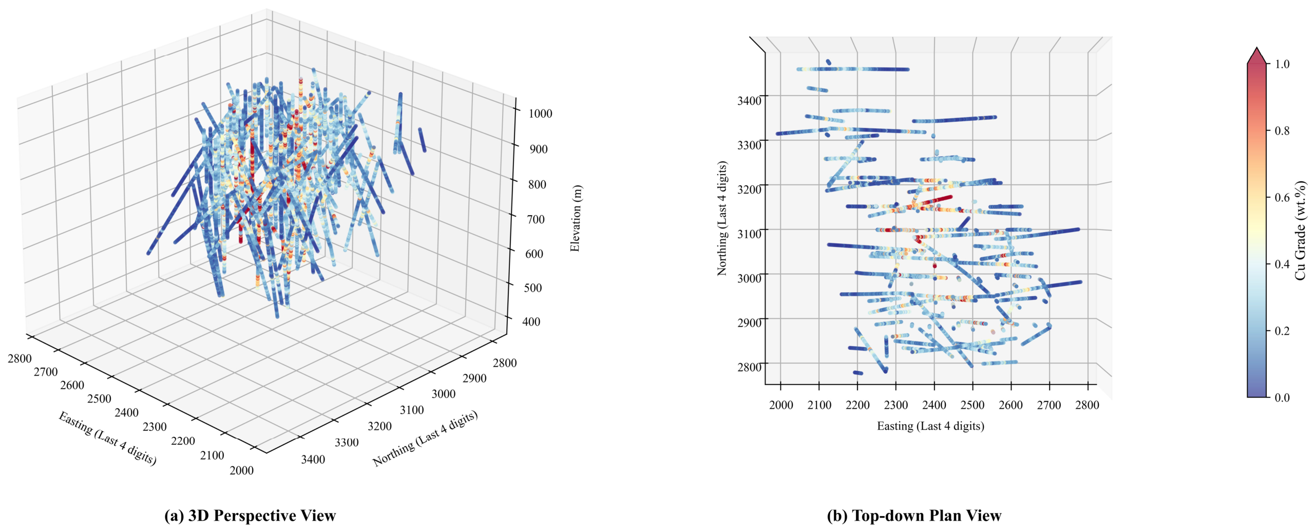
To support the grade modeling of this complex ore body, this study integrated 157 exploration drill-holes (Figure 1). The layout of these drill-holes aligns with the upright cylindrical morphology of the deposit: inclined drill-holes captured the anisotropic gradients at the ore margins, while the remaining vertical holes focused on characterizing the vertical zonation from the potassic to the propylitic zones. Drill-hole depths range from 57 to 450 m, ensuring comprehensive coverage of the shallow oxidized zone and the deep primary sulfide zone. Through systematic sampling of approximately 32,000 m of core intervals and applying a 3-m compositing interval, a grade database comprising 10,668 sample points was constructed. This sample size is sufficient to enable machine learning algorithms to capture localized spatial patterns, ensuring model robustness under non-stationary conditions.

3. Methods

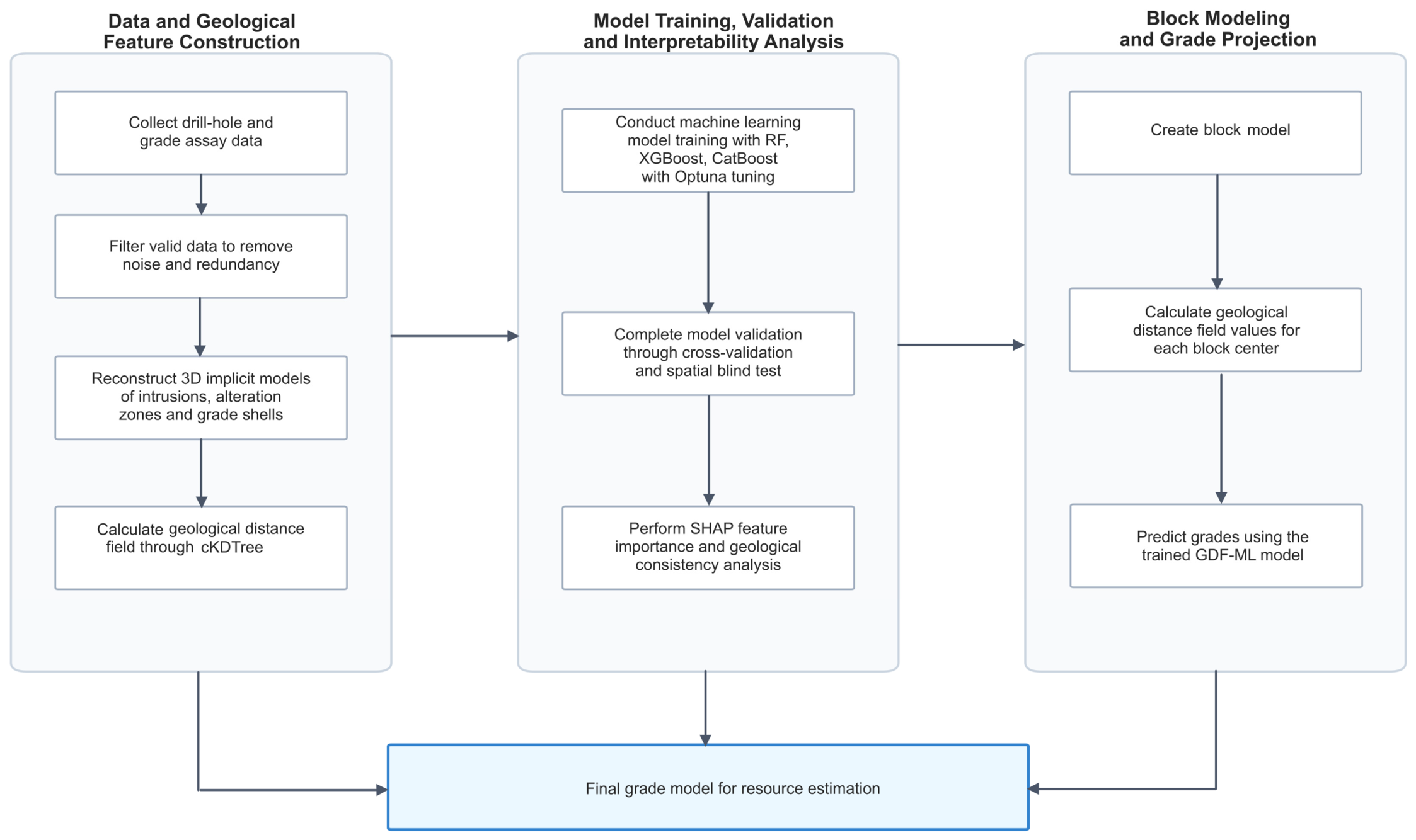
The methodology is structured into three integrated components (Figure 2). First, a set of spatial features is engineered by computing point-wise Geological Distance Fields (GDF), which quantify the relative spatial relationships between drill-hole samples and key geological architecture (e.g., intrusions, alteration zones, and grade shells). Second, the framework is implemented using ensemble learning algorithms—specifically Random Forest (RF), XGBoost, and CatBoost—with hyperparameters optimized via Optuna v4.7.0. To ensure model transparency, SHAP (SHapley Additive exPlanations) is employed to quantify feature contributions, verifying that the predictive logic is fundamentally aligned with established metallogenic principles. Finally, the optimized models are deployed across a 3D block model, where GDF features computed at each block center facilitate a spatially consistent reconstruction of the deposit’s grade distribution.

3.1. Implicit Modeling

The core of this study lies in the integration of porphyry bodies and mineralized domains into a unified mathematical framework via implicit modeling techniques [14,15]. By extracting boundary constraints directly from drill-hole data, this approach moves beyond manual explicit sectional interpretation, representing geological bodies as a topological continuum. This process defines the deposit’s macro-skeleton, which serves as a spatial foundation for subsequent grade modeling.
The internal domains of the porphyry system are modeled as geometric surfaces to represent the spatial distribution of mineralization trends and alteration patterns. These surfaces function as spatial benchmarks for the estimation process. By calculating the minimum distance from each sample point to these interfaces, the discrete geological observations are converted into continuous numerical features. This approach integrates the deposit’s structural geometry directly into the spatial modeling pipeline.
Three-dimensional domains—encompassing lithological units, hydrothermal alteration zones, and grade shells—are reconstructed using implicit radial basis functions (RBFs). This method applies continuous RBF interpolation to discrete geological logging intercepts and composited assay data. Specifically, grade shells are generated by solving implicit equations for surfaces at defined copper cutoff thresholds (e.g., 0.2% and 0.5% Cu). This process yields mathematically defined volumes, providing a representation of the porphyry system’s spatial continuity.
It is important to note that the geometric surfaces generated via RBF implicit modeling function as macro-scale trend indicators rather than as precise boundaries of uniform grade. The geological constraints for lithology and alteration, derived from routine core logging, provide a generalized macro-scale framework. Furthermore, due to the inherent geological nugget effect and short-range stochastic noise characteristic of porphyry systems, raw sample assays near these reference surfaces frequently exhibit grade fluctuations that the RBF shells cannot fully represent. This limitation confirms that the RBF-derived geometry captures the structural and hydrothermal skeleton rather than short-range chemical variations. This spatial discrepancy mathematically justifies the implementation of machine learning algorithms to bridge the gap between macroscopic geometric constraints and localized sample variations.

3.2. Calculation of Geological Distance Fields

To map drill-hole samples into a geologically meaningful scalar field, we define a workflow that calculates the Signed Distance Field (SDF) of each sample relative to the reconstructed geological surfaces. By quantifying the spatial relationship between sample points and these boundary interfaces, we transform discrete point data into continuous field features. This process provides the machine learning models with explicit geometric context, ensuring that the feature space is constrained by the deposit’s structural framework rather than relying solely on raw coordinate-based interpolation.

3.2.1. Geometric Computing Workflow

The reconstruction of the deposit’s structural framework involves the integration of three core elements: iso-grade shells, lithological units, and alteration zones. The workflow follows a three-step spatial engineering sequence:
All expert-defined geological boundaries are utilized as primary geometric references. These 3D surfaces are discretized into high-density point clouds, ensuring that the morphology and curvature of the porphyry system are accurately represented for subsequent spatial queries.
To handle high-volume spatial queries efficiently, we utilized a k-dimensional tree (cKDTree) partitioning algorithm. This indexing structure reduces the computational complexity of nearest-neighbor searches from linear to O ( l o g n ) . For any given sample point, the algorithm efficiently identifies the nearest vertices on the interpreted surfaces. These proximity values are then utilized to compute the point-wise Signed Distance Field (SDF), providing a systematic measure of the sample’s spatial relationship to key geological features.
To distinguish between internal and external domains, a ray-casting intersection test is performed against the water-tight meshes. By evaluating the intersection parity of a virtual ray originating from the spatial point, a sign is assigned to the calculated Euclidean distance. This transformation yields the Signed Distance Field (SDF), which is mathematically defined as follows:
d SDF ( P )   =   sgn ( P ) min P bound Ω P P bound
The orientation sign function, s g n ( P ) , is defined to distinguish the spatial relationship between the point and the geological domain:
sgn ( P )   =   1 P Ω ext   ( exterior )   0 P Ω   ( boundary )   1 P Ω int   ( interior )  
The geometric engineering workflow is executed via a Python v3.13.5-based processing pipeline. Three-dimensional meshes representing geological domains (lithology, alteration, and grade shells) are imported as Wavefront (.obj) files, while drill-hole sample coordinates are sourced from standard database formats (.csv).
The implementation utilizes the Trimesh library for mesh processing and verification of manifold topology. To ensure mathematical consistency, automated hole-filling routines are applied to resolve non-manifold edges. Spatial queries are optimized using NumPy and Pandas for matrix operations, while nearest-neighbor searches are performed via the cKDTree algorithm from SciPy.spatial. To manage computational efficiency, the processing is executed in structured mini-batches. The resulting continuous SDF values are appended to the sample dataset, yielding an integrated feature matrix structured for subsequent regression analysis.

3.2.2. Geological Attribution of the Signed Distance Field

While the mathematical formulation of this workflow is inspired by the Signed Distance Field (SDF) concept commonly used in computer graphics [16,17,18], our implementation focuses exclusively on point-wise distance computation. Instead of generating a global volumetric field, we use this metric to quantify the spatial relationship between individual samples and defined geological boundaries. This approach adapts the SDF from its conventional role as a kernel for implicit surface interpolation [19] into a spatial feature encoder. By mapping each sample’s relative proximity to geological interfaces, the SDF provides high-dimensional features for integration into machine learning, serving as an alternative to its traditional use in volumetric reconstruction.
A fundamental premise of this framework is that geometrically consistent distances from a geological interface reflect similar environmental conditions. In porphyry systems, iso-grade shells and alteration boundaries serve as spatial proxies for thresholds where physical and chemical conditions during mineralization reached equilibrium. Unlike a standard SDF, the sign in a GDF encodes the concentric zonation of the deposit. Consequently, samples sharing similar GDF values relative to these boundaries are treated as occupying analogous positions within the hydrothermal architecture, allowing the model to correlate samples that share similar distal or proximal affinities to the mineralizing fronts.
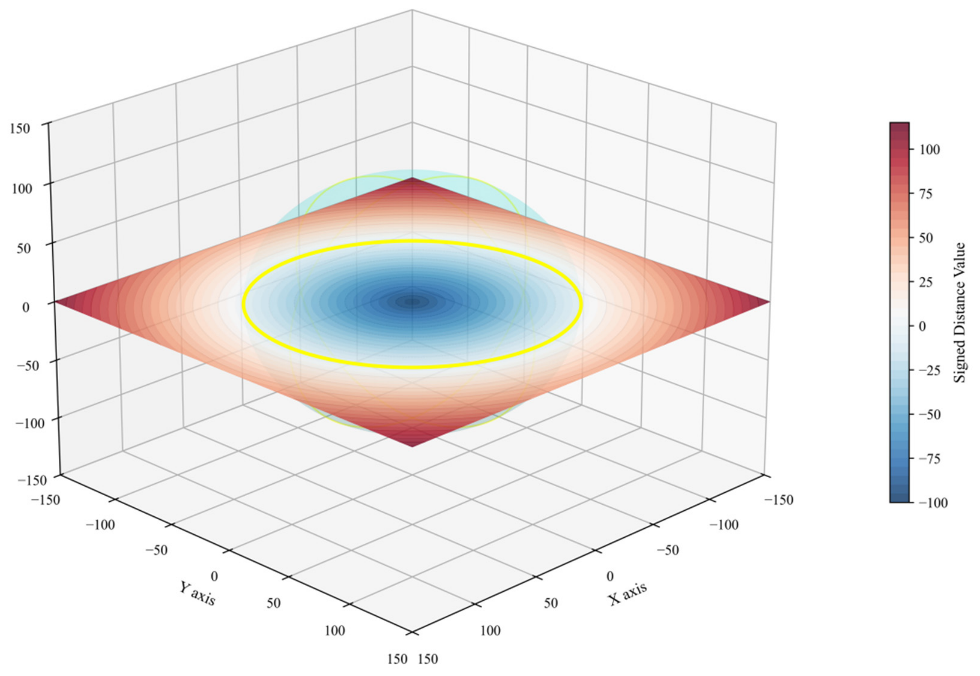
By integrating GDFs derived from multiple sources (grade, lithology, and alteration), the workflow incorporates structural information into the regression process (Figure 3). The combination of these fields allows the machine learning algorithm to evaluate the influence of structural boundaries and host-rock constraints on the target variable. Compared to traditional spatial interpolation, this structured data format enables the machine learning model to better account for the underlying geological controls.
It is important to note that the GDF is derived from expert-interpreted surfaces and functions as a spatial covariate rather than a direct substitute for the target variable. The GDF provides a reference frame that helps the model account for the complex spatial distribution of data. By transforming absolute coordinates into relative distances, the model focuses on the spatial relationship between samples and geological boundaries, rather than purely empirical fitting. This approach improves predictive reliability by incorporating structural context and helps mitigate potential circular reasoning. A detailed assessment of this feature engineering method is provided in Section 5.2.

3.2.3. Evaluation of Feature Independence and Mitigation of Circular Data Leakage

To ensure the GDF-ML framework maintains statistical integrity, it is essential that geometric covariates function as spatial regularizers rather than surrogates for the target variable. In porphyry systems, sample assays are subject to significant local stochastic noise, often referred to as the nugget effect. Therefore, expert-defined grade shells and their derived Geological Distance Fields (GDF) are treated as indicators of broad mineralization trends rather than deterministic boundaries.
To confirm that the machine learning model does not perform an implicit inversion of the grade attributes, we analyzed sample clusters. Our observations indicate that copper grades vary significantly among samples located at equivalent distances from reference shells, and high-frequency grade fluctuations persist even in sample groups with nearly identical GDF values. This confirms that the geometric position vector provides spatial context rather than a direct mapping to the target grade value.
Consequently, the regression algorithm cannot rely on target-lookup routines. Instead, it utilizes a non-linear learning process, employing ensemble tree pathways to reconcile broad geometric contexts with localized empirical data. By treating GDFs as conditioning variables that constrain the conditional expectation of the grade distribution, the framework captures the relationship between structural continuity and localized variance, rather than performing direct numerical retrieval.

3.3. Methods of Machine Learning

3.3.1. Model Selection

We selected tree-based ensemble models for this workflow due to their operational stability and suitability for the structural characteristics of the dataset.
First, our workflow generates correlated GDF features because geological surfaces are often nested or spatially overlapping. Linear models and Artificial Neural Networks (ANNs) are sensitive to this multicollinearity, which can result in unstable coefficient estimates and erratic model convergence. In contrast, tree-based models evaluate features independently during the node-splitting process, making them inherently robust to these correlations.
Second, the recursive partitioning logic in tree-based models aligns better with the data structure of mineral deposits. Porphyry systems often exhibit sharp grade changes across contact boundaries. Unlike ANNs, which rely on smooth activation functions that tend to blur these transitions, decision trees utilize binary splits that capture abrupt changes in grade.
Finally, ensemble techniques such as bootstrapping and sequential residual correction are effective at handling local data variability. These methods allow the model to reconcile assay noise with broader spatial trends. By leveraging these mechanisms, the framework provides a stable baseline for resource estimation without requiring excessive manual data smoothing.

3.3.2. Random Forest

Random Forest [20] acts as a parallelized ensemble of non-linear regressors, utilizing Bootstrap Aggregating (Bagging) to generate robust estimates. In spatial modeling, this architecture maps high-dimensional input features—including GDFs—to grade targets through recursive binary partitioning. By iteratively segmenting the feature space based on spatial proximity to geological interfaces, the algorithm approximates complex mineralization distributions without requiring explicit assumptions of stationarity. Its parallel nature enables high-throughput processing, capturing the structural controls of mineralization across multi-scale estimation grids.

3.3.3. XGBoost

XGBoost represents an gradient boosting framework [21,22] that constructs decision trees sequentially to minimize the residuals of preceding models. Its optimization objective utilizes second-order Taylor expansion and explicit regularization to manage model complexity. In spatial modeling, this sequential refinement allows the model to capture grade attenuation gradients—a characteristic feature near mineralizing fronts. Furthermore, its sparsity-aware splitting mechanism enables consistent feature handling in regions with uneven drill-hole density, facilitating the characterization of non-linear mineralization trends across geological environments.

3.3.4. CatBoost

CatBoost is a gradient boosting framework that utilizes a symmetric tree structure and an Ordered Boosting mechanism [23]. By employing a permutation-based approach to gradient calculation, it addresses the prediction shift often encountered in standard boosting frameworks. Furthermore, its native handling of categorical inputs—using target statistics rather than one-hot encoding [24]—avoids the dimensionality issues associated with encoding lithological and alteration labels. In spatial modeling, these features enable the model to learn non-linear relationships at complex domain boundaries with minimal preprocessing. The symmetric tree structure constrains model complexity, promoting computational efficiency when analyzing large-scale mineralized datasets.

3.3.5. Hyperparameter Optimization via Optuna

To optimize model performance, this study employs the Optuna framework, which implements Bayesian Optimization principles [25]. Unlike exhaustive grid search, Optuna utilizes previous trial trajectories and the Tree-structured Parzen Estimator (TPE) sampler [26] to iteratively narrow the search space toward optimal parameter configurations within a reduced computational timeframe. During the optimization process, the framework monitors performance indicators—such as decision tree depth and learning rate—and employs a pruning mechanism to terminate trial branches that exhibit suboptimal convergence. This data-driven, closed-loop tuning aligns the model with the non-linear features of geological domains while mitigating overfitting risks, thereby supporting the reliability of mineral resource estimation.

3.3.6. Operational Pipeline for Ensemble Training

The operational pipeline for ensemble training and hyperparameter configuration is implemented through a Python-based workflow using standard scientific libraries. Three-dimensional spatial datasets are imported from standardized files (.csv) using Pandas and NumPy. Continuous spatial covariates are compiled into the input feature matrix (X), explicitly including the distance fields derived from multi-threshold grade shells and hydrothermal alteration zones. Copper assays from exploration drill-holes are configured as the target variable (y).
The training sequence systematically evaluates three distinct ensemble regressors: Random Forest, XGBoost, and CatBoost. Hyperparameter configuration is automated via the Optuna framework, utilizing Bayesian optimization principles. The objective function evaluates trial trajectories across a predefined search space, focusing on architectural parameters including maximum tree depth, learning rate, and the number of estimators. Following 15 optimization trials, the framework selects the hyperparameter sets that maximize the coefficient of determination (R2). Optimized model configurations are trained on the dataset and serialized into binary files using the joblib module for deployment.

3.4. SHAP Analysis

To quantify the marginal contribution of spatial features to grade estimation and enhance model interpretability, this study introduces the SHAP (SHapley Additive exPlanations) framework based on cooperative game theory. By calculating the Shapley Value for each input feature, SHAP transforms the “black-box” predictive process of machine learning into a quantifiable attribution analysis [27,28,29]. In the context of geological modeling, SHAP is used to verify that the model’s decision logic is consistent with established geological principles. By observing the contribution trends of grade estimations as they vary with GDF, it is possible to interpret how the specific machine learning model responds to variations in spatial features.
However, it must be emphasized that SHAP analysis explicitly quantifies the internal behavioral characteristics of the mathematical model rather than directly reflecting or empirically proving inherent physical or geological laws. The generated feature–response curves serve as an analytical diagnostic tool to evaluate model alignment with expected mineralization attenuation trends, thereby verifying the empirical plausibility of the model architecture. Furthermore, SHAP identifies the relative importance of various GDF features in their contribution to the final grade, revealing the spatial influence of dominant factors within the trained predictor. Computationally, these attribution calculations and dependency evaluations are implemented using the optimized SHAP Python library v0.50.0 and TreeExplainer.

3.5. Separation and Decoupling Between Geological Framework and Model Training

To establish a scientifically rigorous boundary between spatial conditioning variables and ensemble learning, a strict mathematical decoupling is enforced. Three-dimensional meshes representing lithological units, alteration zones, and grade shells are generated exclusively as macro-scale trend indicators rather than deterministic representations of stationary grade attributes.
Given the intense nugget effect and short-range stochastic noise inherent to porphyry systems, samples at identical spatial Geological Distance Field (GDF) contours exhibit high variance. Because identical distances to a reference mesh map to widely divergent grades, it remains mathematically impossible for tree-based algorithms to deterministically inversely decode or memorize local values via proximity metrics. Instead, the ensemble operates by scanning the deposit space to identify similar multidimensional geometric profiles, utilizing recursive non-linear binary splits to compute the conditional expectation of the grade distribution.
To empirically verify the generalizability of these structural-grade mappings, we implemented three distinct cross-validation (CV) configurations:
Standard Randomized CV (2-fold/5-fold): Establishes a baseline for non-linear fitting under uniform random distributions.
Sequential CV: Preserves the drill-hole logging order to evaluate model stability against systematic structural variations.
Spatial CV: Segments the dataset into separated eastern and western domains. Models trained on one domain are evaluated against the other, ensuring that parameterized correlations remain consistent across distinct spatial zones. Specifically, the spatial partition mitigates the influence of spatial autocorrelation, which often leads to over-optimistic performance metrics in conventional randomized cross-validation.
By integrating these validation regimes, we demonstrate that the regression system prioritizes regional geological trends over localized coordinate artifacts, ensuring the parameterization process remains insulated from data leakage.

4. Model Training and Evaluation

4.1. Implicit Modeling and GDF Construction

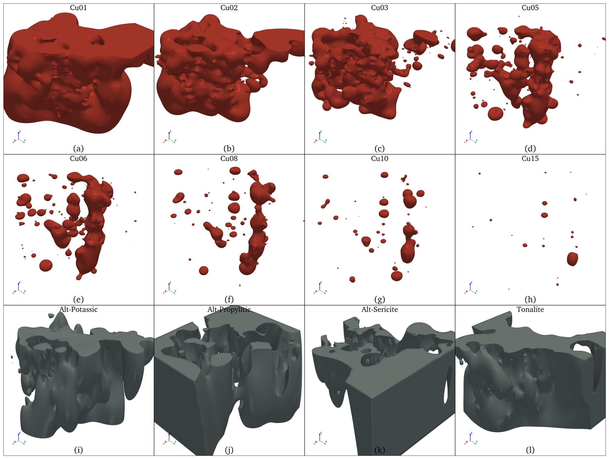
To accurately characterize the wide grade range and complex spatial evolution of the porphyry copper deposit, a multi-threshold constraint strategy was employed to construct implicit models for the tonalite intrusion (Figure 4l), three primary alteration zones (Figure 4i–k), and eight nested mineralization domains (Figure 4a–h; grade thresholds ranging from 0.1% to 1.5%). Based on these discretized volumes, the cKDTree algorithm was utilized to compute point-wise Geological Distance Field (GDF) features for each sample.
The feature nomenclature adheres to geological semantics to ensure interpretative clarity: mineralization domain features are prefixed with NDTS (e.g., NDTS02 for the 0.2% threshold), the intrusion feature is defined as NDTI, and alteration-related features are designated as NDT_Alt_Potassic, NDT_Alt_Propylitic, and NDT_Alt_Sericite.
By adopting a coordinate-free design, the model avoids reliance on absolute spatial positioning (X, Y, Z) and is instead compelled to learn from the intrinsic geometric relationships and hydrothermal gradients inherent in the porphyry system. This ensures that the resulting grade estimations reflect geological processes rather than mere spatial interpolation. This approach mitigates the coordinate memorization effect inherent in XYZ-based models. Unlike raw coordinate inputs that force algorithms to fit absolute sample locations, the framework utilizes structural covariates to characterize underlying mineralization trends [9,30,31,32,33,34].
Categorical features such as lithology and alteration frequently exhibit low sensitivity when predicting continuous grade variables. One-hot encoded representations introduce discrete, step-wise constraints that fail to capture the continuous concentration gradients inherent to porphyry systems. Conversely, the GDF framework represents these gradients via a continuous numerical field, serving as a consistent proxy for the hydrothermal environment. Consequently, categorical parameters were excluded from the feature set to mitigate noise from abrupt boundary artifacts and align the algorithm with the fundamental drivers of grade evolution.

4.2. Model Construction and Validation Strategy

4.2.1. Construction of Model and Validation Based on Shuffled Data

Based on the comparative analysis of the model performance across different validation scales, the results for the GDF-ML framework are described as follows:
The predictive performance of the machine learning models was evaluated using shuffled 5-fold and 2-fold cross-validation (CV) to test for spatial generalization and stability. The Random Forest model demonstrated consistent performance across both 5-fold (Table 1) and 2-fold cross-validation (Table 2) schemes, with R2 values of 0.868 and 0.873, respectively. This stability persisted despite the reduction in training data to 50% in the 2-fold configuration. Furthermore, error metrics remained stable across these schemes, with Mean Absolute Error (MAE) at 0.054 and Root Mean Square Error (RMSE) ranging from 0.098 to 0.099. These results indicate that the model’s predictive performance is insensitive to fluctuations to the volume of training data and the specific partition of spatial data, suggesting that the model identifies mineralization trends derived from the geological architecture rather than relying on local sample clustering.

4.2.2. Construction of Model and Validation Based on Non-Shuffled Data

To evaluate the spatial generalization of the framework, a non-shuffled 2-fold cross-validation was performed based on sequential drill-hole partitions. By excluding entire drill-holes from the training phase, this validation procedure approximates a blind test, assessing the model’s ability to generalize mineralization trends beyond the immediate proximity of training data. Under these conditions, the three ensemble models achieved R2 values of 0.867 (Random Forest), 0.851 (XGBoost), and 0.842 (CatBoost) (Table 3).

4.2.3. Construction of Model and Validation Based on Geographically Separated Data

To evaluate the spatial generalization of the GDF-ML framework, we implemented a 2-fold spatial cross-validation (Spatial CV). The dataset was partitioned into two geographically isolated volumes—the Western and Eastern Domains—using the median Easting coordinate as a physical split line. This validation followed a bidirectional pipeline: in Fold 1, regressors were trained exclusively on samples from the Eastern Domain to project copper grades onto the withheld Western Domain; in Fold 2, the training and test sets were inverted, with models trained on the Western Domain and evaluated against the insulated samples in the Eastern Domain.
The final cross-validation metric represents the mathematical average of these two spatial validation tests. Despite the strict regional insulation and the complete absence of overlapping geographic training constraints, the optimized Random Forest regressor demonstrated substantial structural robustness, maintaining a stable validation baseline with a Spatial CV_R2 of 0.851 (Table 4), a Mean Absolute Error (MAE) of 0.057, and a Root Mean Squared Error (RMSE) of 0.106.
If the regression behavior were primarily driven by local spatial proximity or sample memorization, transferring model parameters across a distinct geographic boundary would result in a significant increase in estimation residuals. The observed stability of the R2 metric (0.851) suggests that the GDF-ML framework does not rely on local coordinate information. Instead, these results indicate that the algorithm utilizes continuous GDF metrics to capture spatially transferable structure-grade relationships.

4.2.4. Selection of Model

Based on the performance metrics across all validation schemes (Table 1, Table 2, Table 3 and Table 4), the Random Forest (RF) model was selected for the final predictive framework due to its generalization stability under stringent spatial testing. While alternative configurations occasionally demonstrated higher training-set variance, the RF model maintained consistent performance across geographically separated validation folds, indicating a low susceptibility to coordinate-based memorization. By leveraging the GDF-driven framework, the RF model functions as an inferential engine, translating continuous numerical fields into grade estimations. This approach ensures that the model captures generalized mineralization patterns rather than memorizing individual sample locations.
The reported R2 of 0.851 is interpreted as an index of geological information extraction rather than a measure of deterministic goodness-of-fit. By utilizing GDFs as spatial constraints, the framework operates as a filter, allowing the regressor to distinguish between stochastic micro-scale noise and structurally driven grade trends. This mitigates the smoothing effect inherent in traditional methods, positioning the R2 as a quantitative measure of the geological information captured and retained by the model.

4.3. Feature Sensitivity and Structural Robustness Analysis

To further evaluate the dependency of the GDF-ML framework on the precision of the input geological structures, a structural sensitivity analysis was conducted. This test aimed to determine how local perturbations in the foundational Geological Distance Fields (GDF) influence the model’s ultimate predictive accuracy.

4.3.1. Structural Perturbation Experiment

To assess the sensitivity of the GDF-ML framework to geometric variations, a structural perturbation experiment was conducted. In this procedure, 20% of the original sample data were randomly withheld, and the GDFs (including grade shells, lithology, and alteration domains) were reconstructed using only the remaining 80% of samples. This introduction of localized spatial perturbations provided a basis to evaluate the model’s dependency on the precise geometry of the GDFs. The optimized Random Forest model was subsequently applied to predict grade values for the withheld 20% dataset using these perturbed features. This experiment isolates the framework’s reliance on geometric input precision, evaluating whether the model maintains predictive stability when the underlying structural constraints are subject to localized variability.

4.3.2. Sensitivity Results and Analysis

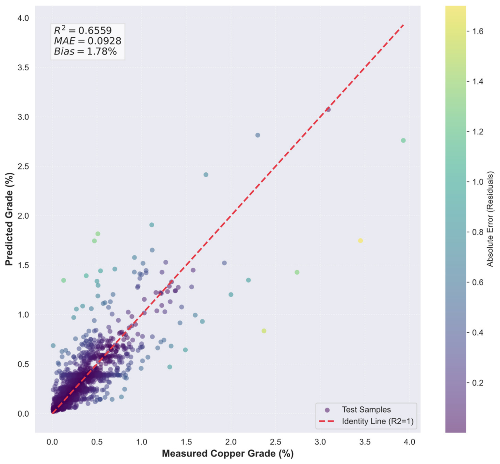
As shown in Figure 5, the independent test set performance declined compared to the internal cross-validation results, with R2 decreasing to 0.6559 and MAE increasing to 0.0928. This sensitivity to localized geometric perturbations indicates that the Random Forest model relies heavily on the structural fidelity of the GDFs. Specifically, when sample points are withheld from the construction process, localized shifts in the distance fields—such as NDTS05—induce minor structural inaccuracies. These geometric variations propagate through the model’s feature space and reduce grade estimation precision, confirming that the framework’s predictive accuracy is intrinsically coupled to the high-resolution geometric representation of the deposit’s geological structures.

4.3.3. Implications for Geological Modeling

These results clarify the model’s operational logic, as the performance observed in the primary validation (R2 = 0.868) is contingent upon the structural integrity of the geological domains. The model’s sensitivity to geometric perturbation confirms that the GDFs function as spatial constraints rather than auxiliary variables. Consequently, the predictive output is fundamentally tied to the resolution and accuracy of the geological interpretations used to construct these fields. This reinforces the necessity of maintaining high-fidelity structural models, as the accuracy of the grade estimation framework is intrinsically coupled to the precision of the deposit’s interpreted spatial distribution.

4.3.4. Rationale for Validating on a Complete GDF Framework

Both shuffled and non-shuffled cross-validations were performed within a fully established GDF framework. Retaining the complete framework during validation is based on the following:
Structural Consistency: In high-heterogeneity deposits, removing entire drill-holes modifies the reconstructed GDF scaffold. This prevents an objective assessment of the model’s sensitivity to refined geometric variations.
Global Structural Logic: Unlike local interpolation methods, the GDF-ML framework uses a global structural approach. Predictions are based on the sample’s position within defined geological constraints rather than local proximity, ensuring estimation is driven by the system’s topological logic.
Geometric Sensitivity: Withholding 20% of individual samples introduces controlled, local perturbations while maintaining the global structure. The observed R2 of 0.6559 confirms that the model is sensitive to fine-scale geometric accuracy. This validates that the high precision in primary runs (R2 of 0.868–0.873) is derived from resolving complex, non-linear relationships between grade and distance fields.

4.4. SHAP Interpretation

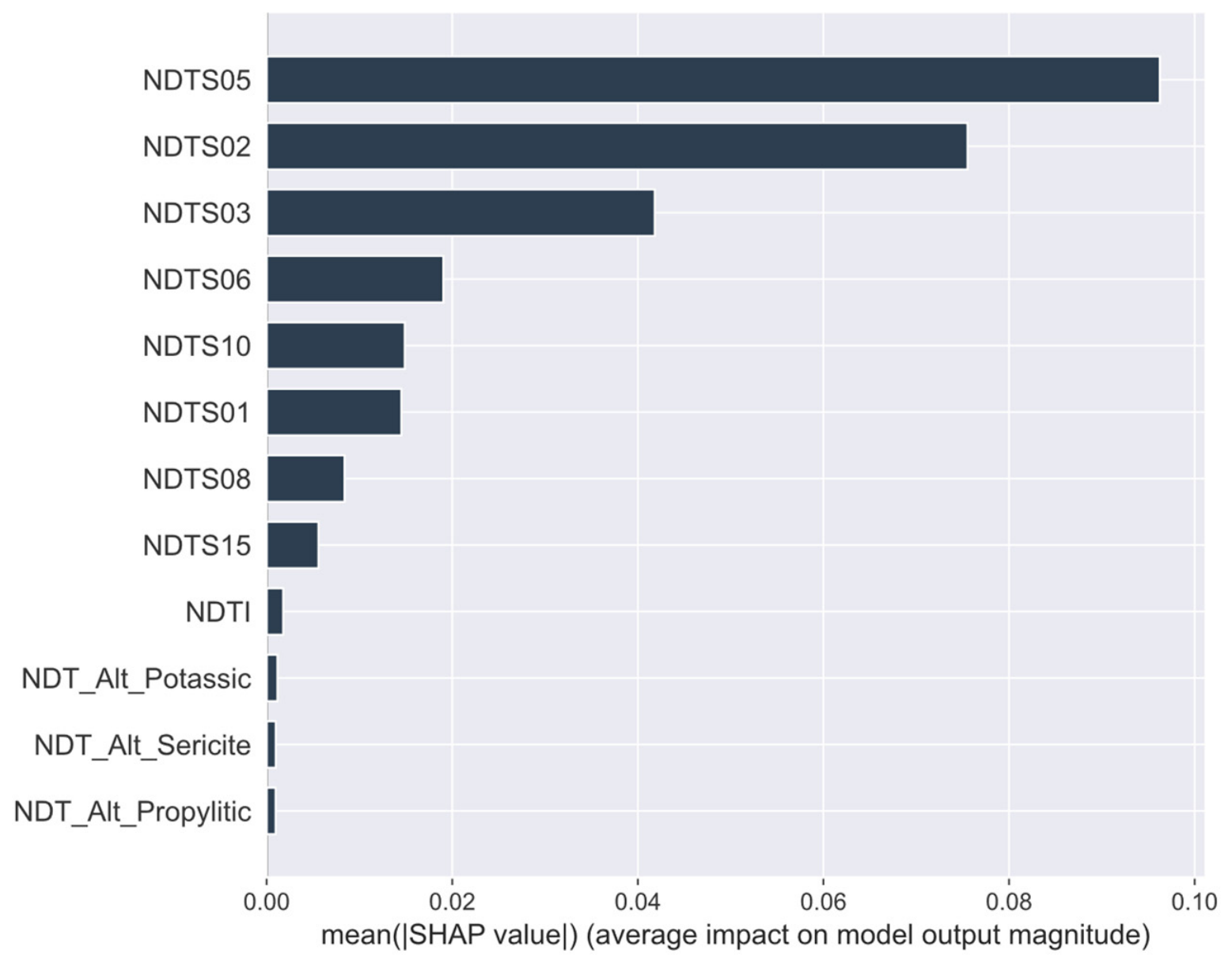
The SHAP feature importance analysis (Figure 6) quantifies the relative contribution of each input variable to the model’s decision-making process, identifying NDTS05 and NDTS02 as the dominant splitting criteria. This hierarchical importance confirms that the continuous distance variables, derived from macroscopic grade domains, serve as the primary drivers of the model’s output. The reliance on these specific features validates that the expert-defined grade shells effectively constrain the spatial distribution of copper grades within the model. Consequently, the feature-attribution plot provides a quantitative diagnostic of how the GDF-ML framework leverages these geometric constraints to define its estimation pathways, reinforcing the model’s reliance on structural–geological logic over mere spatial indexing.
Figure 6 reveals that the statistical contribution assigned to the alteration features (NDT_Alt) remains significantly lower than that of the grade shell features (NDTS). This statistical pattern indicates that within the empirical variance minimization process, the tree-based optimization algorithm assigns lower splitting priority to these broad-spectrum spatial envelopes. Because the macroscopic alteration zones (e.g., Potassic, Sericitic, and Propylitic) encompass massive contiguous volumes with high regional spatial continuity, their calculated scalar field metrics lack the local gradient variations necessary to significantly reduce regression residuals during individual node partitioning sequences.
Consequently, the global minimization criteria of the ensemble learning loop automatically assign lower selection priority to these background features. This mathematical filtering behavior demonstrates that the model’s predictive pathways dynamically prioritize continuous geometric indicators derived from the grade shells—which possess a higher capacity to explain localized variance—over uniform regional features. By reducing parameter dependency on these secondary variables, the mapping framework optimizes its splitting sequences based strictly on the localized numeric sensitivity of the features within the training database.
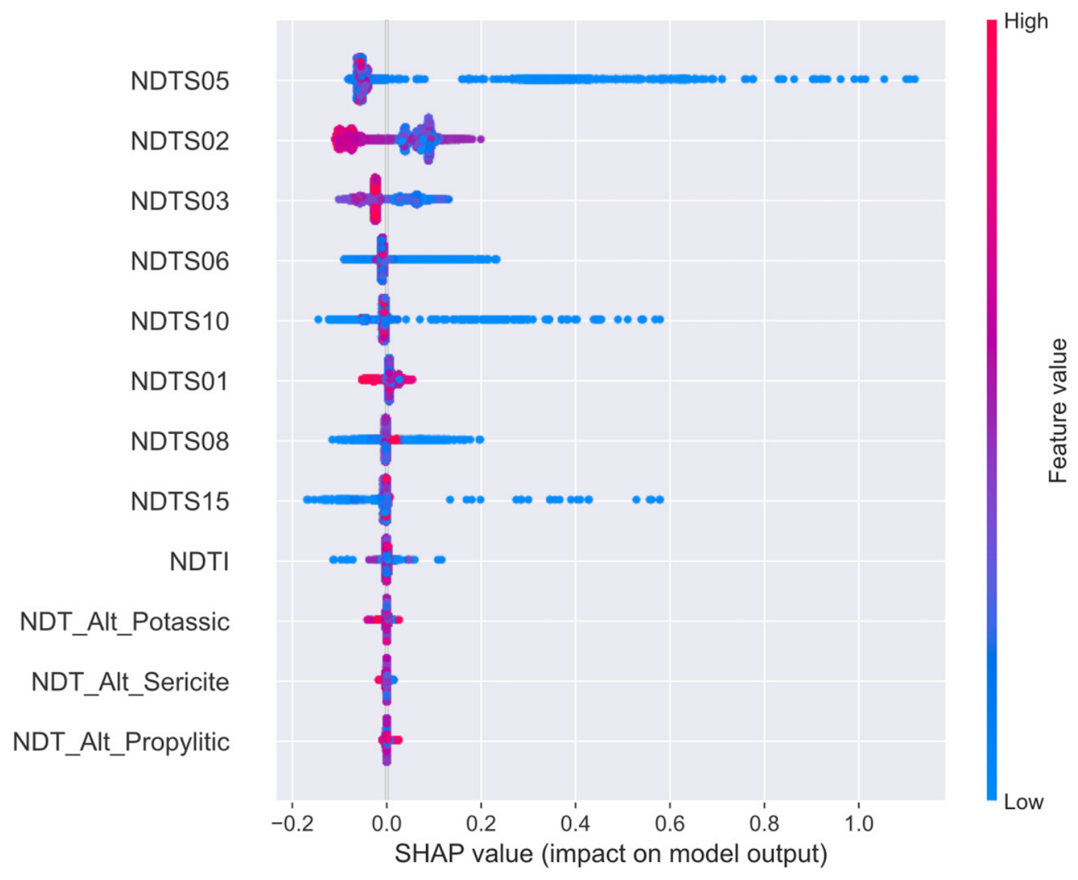
The SHAP beeswarm plot (Figure 7) quantifies the non-linear response behavior between the input Grade Shell features (NDTS) and the output regression vectors. This algorithmic behavior is most evident in the top-ranking covariate, NDTS05, where the calculated SHAP attribution values exhibit a pronounced asymmetric long-tail distribution along the positive axis. Specifically, lower feature values—represented by the blue dots—trigger a rapid, non-linear escalation in SHAP values. Conversely, high feature values—represented by the red dots—remain tightly clustered adjacent to the zero-impact baseline.
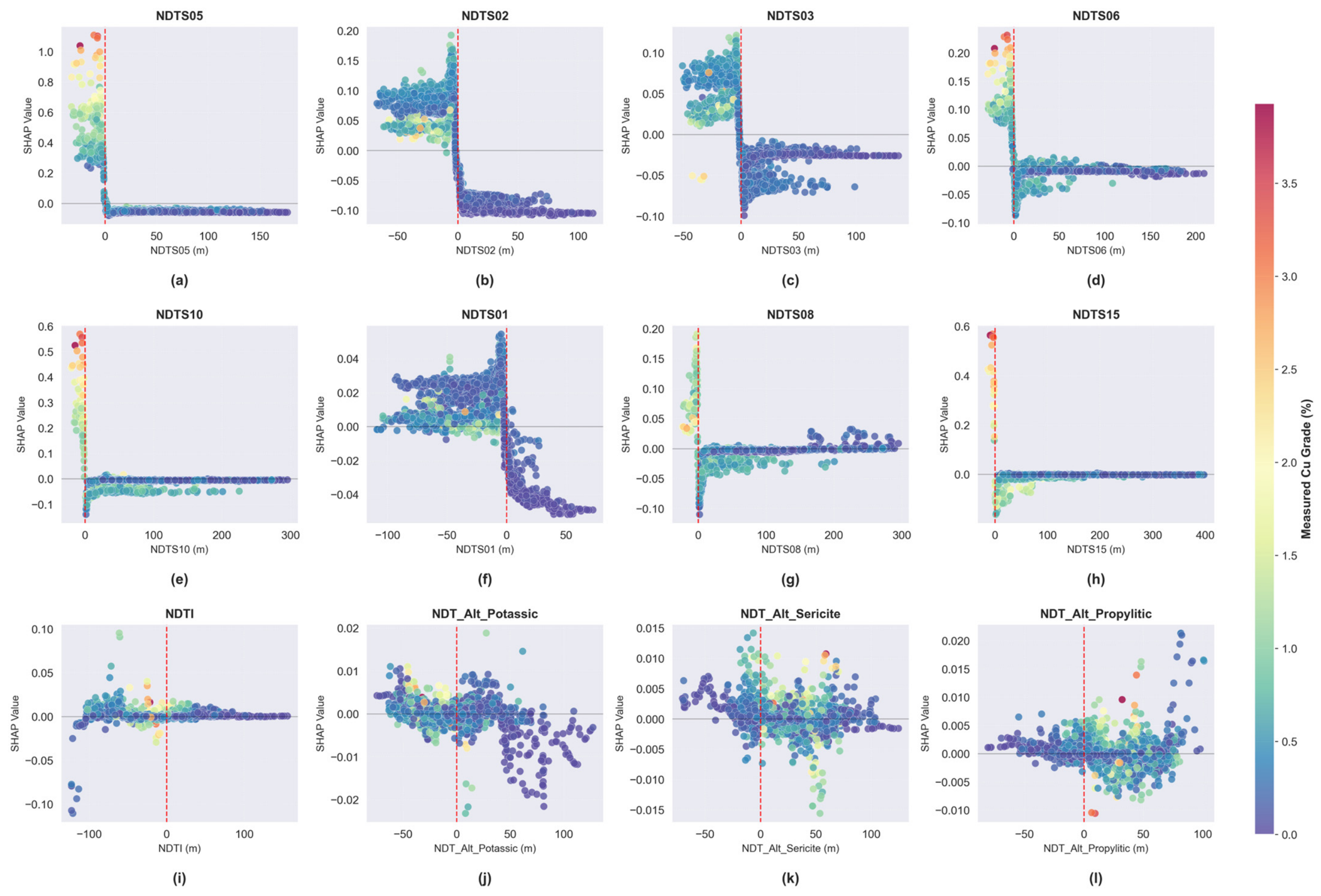
The SHAP dependence plot matrix (Figure 8) illustrates a step-like transition across the numerical zero-point intercept of each grade feature. As the distance field metric shifts from positive to negative values—representing a sample coordinate’s spatial transition into the interior frame of a specific shell—the localized marginal contribution to the estimation output exhibits an abrupt shift, followed by non-linear fluctuations or numerical decay. This precise lock-on at the geometric interfaces demonstrates the tree-based ensemble’s sensitivity to predefined feature boundaries, capturing the numerical truncation adjustments inherent to the input configuration.
This interfacial sensitivity is a function of the gradient alignment achieved within the multidimensional feature space. The grade shell features (Figure 8a–h) predefine a set of geometric trajectories that partition the space domain. When these continuous geometric covariates align with the variance boundaries of the target grades, the regression algorithm utilizes highly prioritized binary splits to minimize the global loss function. This statistical mechanism transforms discrete spatial reference boundaries into continuous, feature-driven gradient responses within the mapping network.
Consequently, this multivariable feature interaction allows the machine learning architecture to parameterize localized gradient fluctuations based strictly on empirical numeric constraints. This behavior confirms that the trained model’s decision pathways consistently rely on the provided grade shells to regulate estimation paths, ensuring that the final output honors the spatial configuration and continuous trends of the copper grades.
While the grade shell metrics (NDTS) exhibit pronounced threshold-like transitions, the other four structural parameters (e.g., NDTI, NDT_Alt) show less significant variation in their SHAP values (Figure 8i–l), with most contributions concentrated near zero. This suggests that these features act primarily as subtle regulatory constraints rather than primary drivers, providing localized adjustments to the model’s estimation paths without triggering large-scale shifts in predictive weight. This hierarchical feature contribution pattern highlights the model’s ability to prioritize primary mineralization controls while utilizing secondary features for localized refinement.
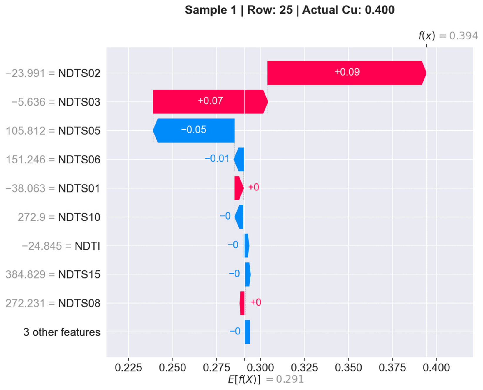
Figure 9 presents a SHAP waterfall plot for a representative sample (Actual Cu: 0.400%), illustrating the localized numerical evaluation pathway of the trained regressor. Starting from the dataset base value of E[f(X)] = 0.291, the final model output of f(x) = 0.394 is primarily driven by the sample’s positioning relative to the 0.2% and 0.3% grade shells (NDTS02 and NDTS03), which contribute +0.09 and +0.07, respectively, to the grade value. Conversely, because the coordinate attributes place the sample outside the 0.5% grade shell (NDTS05 = 105.812), the algorithm applies a localized inhibitory adjustment of −0.05 to refine the output vector. This sample-level decomposition demonstrates the model’s localized estimation behavior, showing how the tree-based regression pathways integrate multiple grade shell boundaries simultaneously to adjust individual grade calculations.

4.5. Grade Model Estimation and 3D Spatial Analysis

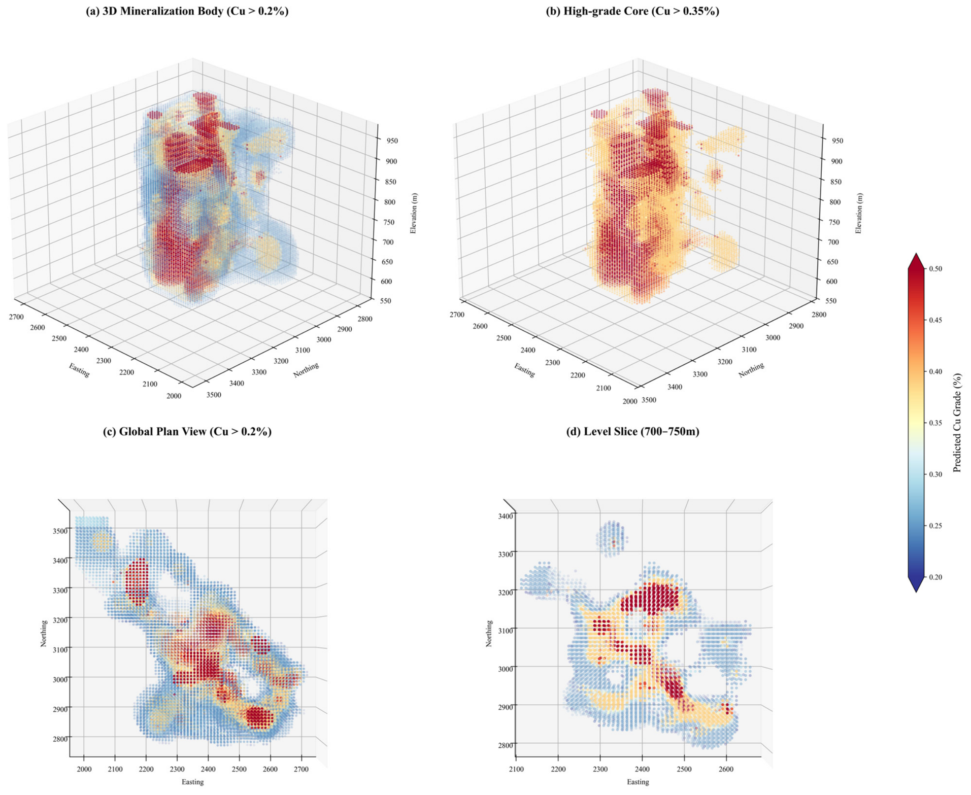
A 3D block model with a unit cell size of 10 m × 10 m × 10 m was constructed across the deposit as the framework for spatial estimation. Utilizing the cKDTree algorithm, spatial distance metrics relative to the predefined grade shells (NDTS) were calculated for each block center. These geometric features were then processed through the trained Random Forest (RF) model to generate the final 3D copper grade estimations across the block grid.
By visualizing voxels with calculated values above the 0.2% Cu threshold (Figure 10a), the block model illustrates the spatial configuration of the estimated grade distribution. The 3D visualization outlines the macroscopic geometric contours of the high-value zones across the grid framework. Specifically, the generated block model reproduces a lower-grade internal zone surrounded by higher-grade domains, which aligns structurally with the concentric spatial topology predefined by the input grade shells. This pattern demonstrates that the tree-based optimization algorithm consistently utilizes the multi-threshold continuous distance covariates to regulate its spatial estimation pathways across different coordinate zones.
When the visualization threshold is restricted to values above 0.35% Cu (Figure 10b), the model delineates the localized configuration of the highest predicted grade zones. Rather than exhibiting severe spatial smoothing effects, the block model parameterizes irregular geometric morphologies and discrete high-value centers within the grid. This numerical capacity ensures that localized spatial heterogeneity is preserved during the spatial prediction process, reflecting the localized numeric sensitivity of the trained ensembles to the structural constraints within the input database.
Through the integration of global plan views (Figure 10c) and horizontal level slices (Figure 10d), the block model documents consistent grade trends across different spatial resolutions. The global perspective reveals the broad-scale horizontal continuity of the predicted grades, while the localized horizontal dissection exhibits the continuous trends of the high-value centers within the 700–750 m elevation framework. This multi-scale consistency—from regional trends to localized grid details—confirms that the mapping workflow operates as a structurally bounded numerical tool, outputting a stable and geologically consistent spatial baseline that honors the predefined geometric constraints.

5. Discussion

5.1. Acknowledgment of Target-Informed Priors and Methodological Limitations

The GDF-ML framework relies on grade-shell-derived distance fields (GDFs) to characterize structural mineralization controls. It is essential to explicitly acknowledge that these grade shells are, by design, target-informed. As they are constructed from exploratory drilling data, the geometric frameworks they define are inherently linked to the spatial distribution of known mineralization. This relationship requires a clear distinction between the use of these shells as “spatial containers” and the objective of the machine learning regression.
It is necessary to clarify that the use of grade-shell-derived GDFs does not constitute circular reasoning. In our framework, the grade shell provides the structural container for the mineralized system, establishing a spatial domain within which the model performs non-linear inference. The regression engine does not lookup grade values; rather, it performs mapping within a structurally bounded search space. The GDF functions as a spatial regularizer, constraining the engine to respect established geological domains and preventing the smoothing artifacts common in unconstrained interpolation.
However, the validation of this framework is subject to specific limitations:
  • Validation Strategy Constraints: A fundamental limitation of the current validation pipeline is that cross-validation is inherently performed within the context of the established structural GDF framework. Because the GDFs themselves encapsulate the geometry derived from the complete deposit dataset, the evaluation measures the model’s ability to interpolate within these defined structures, rather than its capacity to predict mineralization in the absence of such structures. Consequently, our cross-validation reflects the model’s precision as an internal estimation tool—optimizing grade distribution within known geological constraints—rather than its standalone predictive performance in a completely blind scenario without structural priors.
  • Dependency on Structural Interpretation Accuracy: The framework’s predictive performance is intrinsically bounded by the accuracy of the initial structural interpretation. Where these interpretations are incorrect or incomplete, the model’s performance may decay. In this context, performance metrics serve as a diagnostic indicator of structural inconsistency rather than purely a failure of the machine learning engine.
  • Reconciliation vs. Predictive Forecasting: The validation strategy presented herein focuses on the model’s effectiveness in reproducing known mineralization patterns (reconciliation) within an established framework. Consequently, this architecture is best defined as an expert-constrained optimization tool designed to enhance resource estimation precision, rather than a standalone predictive model intended for virgin, undrilled volumes devoid of prior structural guidance.

5.2. Conceptual Validity and Mitigation of Circularity

While the target-informed nature of the GDFs is acknowledged, a critical mathematical distinction must be maintained between this geometry-bounded configuration and the structural target leakage typically encountered in unconstrained machine learning workflows.
The reference grade shells function exclusively as macroscopic geometric constraints designed to accommodate the severe spatial non-stationarity and structural anisotropy characteristic of porphyry systems. They encode the spatial topology of geological domains rather than providing deterministic grade values to the estimators. Crucially, a sample coordinate sharing an identical distance metric relative to a given shell boundary does not possess a uniform or predictable metal concentration. Extensive empirical within-shell grade variance is observed throughout the database, where neighboring samples located along identical geometric contours exhibit distinct high-frequency fluctuations and stochastic jumps due to the intense localized nugget effect.
Because widely divergent copper values map to identical numerical distance metrics within the input feature matrix, the tree-based ensemble models cannot execute a deterministic lookup routine or retrieve a hidden target label. Instead, the regression algorithm evaluates the GDF metrics as coordinate-free spatial references to parameterize the localized gradient decay relative to the structural boundaries. This logic is empirically validated by the perturbation experiments in Section 4.3; when the global geometric integrity of the GDF constraints is slightly distorted near withheld data points, the predictive capacity undergoes a significant decline. This performance drop serves as a diagnostic indicator that the ensemble pathways do not mechanically memorize local grades, but remain strictly conditional on the fine-scale geometric precision of the initial structural models.
Furthermore, the spatial cross-validation—wherein the networks are trained on the eastern domain and evaluated exclusively within the completely insulated western domain—maintains a stable performance baseline. This regime indicates that the learned non-linear relationship between continuous geometric distance and conditional grade expectation generalizes across geographically independent zones, verifying the spatial translation invariance of the regression logic. Collectively, these results justify framing the GDF-ML framework as a geologically guided, expert-constrained spatial regularizer rather than an unconstrained or circular predictor.

5.2.1. Statistical Evaluation of Input Feature Attributes

The operational mechanism of tree-based ensemble models ensures that all input spatial structures are evaluated strictly as continuous numerical covariates during the optimization process. The algorithm operates without any predefined semantic assumptions regarding the geological origin of any specific input field—whether a covariate represents a calculated distance to an interpreted grade shell, a lithological contact, or an alteration boundary.
From an estimation perspective, these continuous distance metrics function exclusively as numerical scalar fields that partition the three-dimensional coordinate space. The statistical correlation between these distance vectors and the target assay values is determined through the iterative minimization of the global loss function during the training phase. Rather than executing a deterministic database retrieval or an attribute lookup based on historical categories, the optimization process evaluates the empirical distribution between the input variables and the continuous target data. Consequently, the feature weights assigned to specific distance covariates reflect their statistical capacity to explain global variance under empirical data constraints, rather than an architectural dependency.

5.2.2. Spatial Distance Covariates as Geometric Constraints

The calculated distance fields do not function as direct numerical proxies for ore grade; instead, they serve as continuous spatial variables that provide relative geometric positioning. While the boundaries of the reference grade shells are constructed from geological interpretations, the distance calculation converts these discrete surfaces into a continuous scalar framework across the deposit. The regression algorithm does not directly reproduce the spatial envelopes; rather, it fits the spatial gradients and localized anisotropy of the continuous grade values relative to these geometric references. This approach provides a structural constraint to the statistical model, minimizing the risk of generating chaotic, unconstrained spatial artifacts that can occur in purely data-driven interpolations. The final estimations reflect the non-linear distribution of copper grades evaluated conditional on this spatial framework.

5.2.3. Structural Alignment and Feature Hierarchies

The SHAP attribution analysis indicates that distance covariates derived from interpreted grade shells exhibit higher relative weights than those derived from macroscopic lithological or alteration boundaries. This variation in global feature contribution reflects the statistical alignment between specific geometric frameworks and the spatial distribution of assay metrics:
  • Identification of Primary Statistical Drivers: The higher relative weights assigned to the grade-shell distance fields indicate that the regression algorithm prioritizes these continuous spatial variables to capture global variance. Within the ensemble optimization process, the algorithm assigns greater splitting priority to the geometric frameworks that exhibit the strongest statistical correlation with the continuous target variable, thereby aligning the numerical framework with the dominant spatial controls of the deposit.
  • Statistical Implication of Secondary Covariates: The lower relative importance scores associated with the lithological or alteration distance fields suggest a weaker direct spatial correlation with localized grade variations at the scale of observation. The model’s capacity to discount these redundant dimensions suggests that the regression pathways can differentiate between primary geometric correlates and broader geological background contexts, providing an empirical basis for assessing feature relevance under joint data constraints.
  • Feature Redundancy and Model Stability: Crucially, the inclusion of these secondary geometric variables does not degrade cross-validation stability or lead to numerical variance inflation. Instead, these secondary fields function as continuous spatial constraints during node partitioning. By incorporating multiple continuous spatial distance inputs, the workflow evaluates the target variable across overlapping geometric domains, which assists in constraining estimations within bounded volumetric limits. Even with minimal attribution weights, these features provide a structural reference that reduces unconstrained mathematical extrapolation in sparse data regions, ensuring that the final output remains consistent with the generalized geological context of the deposit.

5.3. Analysis of Non-Linear Feature Interaction and Variable Attribution

To evaluate the mathematical relationships within the regression framework and examine whether the algorithm relies on local positional memorization of the reference boundaries, this section analyzes the joint feature interactions using SHAP dependency distributions.

5.3.1. Evaluation of Spatial Non-Linearity vs. Linear Interpolation

If the tree-based regression model were restricted to localized numerical proximity effects, its predictive pathways would align with a conventional piecewise linear interpolation along a single dimension. Under such a localized assumption, the estimation for a given target spatial volume would be dictated almost exclusively by the two immediate bounding covariates (e.g., the closest proximal grade-shell distance fields). Consequently, the regression pathways would demonstrate statistical decoupling from distal structural variables, such as the calculated distances to the intrusion stock (NDTI), peripheral alteration zones (NDT_Alt), or the broader low-threshold mineralization envelope (NDTS01).

5.3.2. Multivariable Feature Interaction and Joint Attribution

The SHAP dependency distributions (Figure 8) indicate a combined, multivariable inference mechanism within the regression workflow. The predicted grade value for a given spatial location represents the integrated output of all input continuous covariates—including the multi-threshold mineralization domain distances (NDTS), the lithological contact distances (NDTI), and the alteration domain distances—acting simultaneously through the ensemble tree pathways. This joint evaluation pattern indicates that the model estimates grade variations based on the intersection of multiple spatial boundaries rather than executing a localized linear lookup between two immediate adjacent surfaces.
The vertical dispersion observed within the SHAP dependency plots—where varying SHAP attribution values occur at identical distance metrics—indicates that the marginal contribution of a specific distance covariate is conditional on the values of the remaining spatial features. This variation suggests that the algorithm evaluates the spatial positioning vectors as a continuous multi-dimensional coordinate vector. Consequently, the reference grade shells and structural boundaries do not serve as deterministic labels, but function as simultaneous spatial constraints that anchor the non-linear regression pathways, reducing unconstrained mathematical variance in the presence of short-range stochastic noise.

5.3.3. Spatial Compatibility and Multivariable Regression Consistency

The observed feature interaction within the multivariable regression framework reflects the statistical covariance of the overlapping continuous spatial inputs. While the machine learning model operates strictly on mathematical variance reduction, the joint weighting assigned to the superimposed geometric fields—including the lithological contact distances (NDTI), alteration domain distances (NDT_Alt), and multi-threshold grade shell distance covariates—corresponds to the empirical spatial configuration where multiple geological controls intersect within the porphyry system.
This localized covariate interaction indicates that the algorithm evaluates the spatial inputs as a continuous, cumulative multi-dimensional vector rather than isolating individual geometric surfaces into independent spatial segments. By assigning joint splitting priorities to these spatial covariates, the non-linear regression pathways conform to the spatial continuity of the mineralized zones. This statistical alignment between empirical data fitting and the generalized spatial distribution of the porphyry architecture indicates that the framework’s predictive stability is supported by geometric consistency, ensuring that the final grade estimation honors the broader multi-stage spatial configuration of the deposit.

5.4. Unified Spatial Regression and Operational Integration Analysis

The GDF-ML framework integrates multi-scale spatial constraints within a unified regression architecture while maintaining consistency with generalized geological domains. Conventional geostatistical applications frequently rely on independent spatial partitioning, which requires individual variogram modeling and the localized adjustment of search ellipsoids for disparate lithological units or grade shells. This compartmentalized approach can be computationally demanding and is occasionally susceptible to artificial boundary discontinuities or “edge effects” at domain interfaces, which may misrepresent the continuous spatial gradations inherent in the mineralization system.
  • Covariate-Based Grading vs. Hard Domaining: The continuous distance fields derived from GDF mapping provide domain-wide spatial constraints across the entire deposit volume, minimizing the reliance on manual sub-domaining. Consequently, the requirement for individual variogram fitting within isolated structural blocks is minimized; the regression algorithm characterizes the transitional gradients between the higher-grade core and the peripheral mineralized halos based entirely on the continuous feature space.
  • Integrated Regression Framework via Continuous Features: A operational advantage of the GDF-ML workflow is its capacity to synthesize multiple spatial domains into a single regression envelope. Rather than decomposing the deposit into independent, hard-bounded sub-domains for isolated interpolation, the workflow evaluates the mineralized system within a unified feature space. By encoding structural controls into continuous distance covariates, the model accounts for localized variations and grade gradients within a globally consistent coordinate framework. This continuous approach allows the generalized geological transitions—extending from the high-temperature core to the peripheral alteration domains—to be evaluated as a coherent trend, mitigating the operational burden of managing fragmented, independent sub-estimation files while maintaining the geometric consistency of the 3D block estimates.
  • Sensitivity to Initial Interpretative Constraints: Despite reducing the necessity for manual geometric partitioning, the GDF-ML framework is not an unconstrained, purely data-driven mechanism; instead, its mathematical performance remains highly dependent on the initial delineation of the reference geological structures. The feature construction phase requires input from exploration geologists to translate multi-scale structural data into representative distance variables. If systematic errors exist within the initial structural interpretation relative to the true subsurface distribution, the regression workflow will inevitably propagate these geologically defined biases into the final estimation outputs. Therefore, while this workflow minimizes repetitive manual partitioning steps, its performance relies strictly on the fidelity and accuracy of the conceptual geological model, shifting the engineering focus from empirical variogram tuning toward rigorous structural model validation.

5.5. Comparison Between GDF-ML and Ordinary Kriging

It is important to note that the R2 metrics of the GDF-ML framework and conventional geostatistical methods reflect distinct optimization targets. Conventional approaches, such as Ordinary Kriging, focus primarily on minimizing localized estimation variance, which naturally aligns the resulting block values closely with the nearby sample data. In contrast, the GDF-ML framework operates on global variance reduction, using multi-scale distance fields as structural constraints to maintain geological boundaries and grade gradients. Because these two methodologies utilize different mathematical formulations, their R2 values are not directly comparable. Therefore, rather than relying solely on a single statistical coefficient, this study evaluates the model’s operational performance through a multi-criteria approach, combining regional trend consistency and industrial reconciliation bias to ensure reliability for long-term mine production planning.

5.5.1. Ordinary Kriging Configuration and Variogram Parameterization

To establish a comparative baseline, an Ordinary Kriging (OK) workflow was configured using an anisotropic variogram model. The spatial continuity of the copper assays was characterized via a Spherical theoretical function, exhibiting directional anisotropy consistent with the primary hydrothermal orientation of the porphyry system. The fitted experimental variogram exhibits a Major Axis range of 147.6 m along the vertical vector, conforming to the structural elongation of the mineralized core, while the Semi-major and Minor axes ranges were determined to be 93.28 m and 54.95 m, respectively. A notable geostatistical attribute of this dataset is the normalized nugget effect of 0.6793, which represents approximately 55.5% of the total sill value.
This high nugget-to-sill ratio reflects significant short-range random variability within the sampling intervals. In data environments exhibiting high-frequency variation, the localized linear combinations of Ordinary Kriging typically output a smoothed spatial distribution, which inherently limits the reproduction of localized extreme values. This statistical characteristic provides a standard comparative context for evaluating the non-linear regression framework, which utilizes continuous geometric distance covariates to characterize these localized spatial transitions.

5.5.2. Trend Characterization vs. Numerical Interpolation

Conventional geostatistical methods rely on localized numerical autocorrelation parameters derived from spatial distance intervals. In contrast, the expert-constrained regression framework models the assay distribution using continuous geometric coordinates derived from multi-scale structural boundaries. When the normalized nugget effect is high and adjacent samples exhibit low short-range spatial correlation, the regression algorithm utilizes global loss minimization to fit an expected trend based on the input distance covariates, rather than matching localized high-frequency fluctuations. This alternative approach incorporates the vertical continuity of the porphyry structure within the estimation workflow across multiple spatial scales, providing a geometry-conditioned mathematical representation for non-stationary grade attributes in high-variance systems.

5.5.3. Analysis of Statistical Proximity Effects Under High Spatial Variance

Porphyry systems frequently exhibit pronounced internal variance and constrained variogram ranges, indicating that individual assays possess limited spatial correlation with adjacent samples beyond short intervals. Under these short-range correlation constraints, localized linear interpolators allocate dominant mathematical weights systematically to the nearest sample points. While this proximity dependency honors localized sample values within dense data clusters, the resulting output primarily reflects localized piecewise numerical variations rather than the broader macroscopic trend.
In the absence of geometric constraints, localized linear estimations may incorporate short-range stochastic variance directly into the regional spatial distribution, occasionally leading to localized discontinuities across the block grid. In high-variance systems, evaluating estimation methodologies benefits from analyzing whether the spatial continuity of the block model aligns with the macroscopic geological architecture, rather than relying exclusively on localized statistical metrics.

5.5.4. Structural Constraints as Regularizers

The GDF-ML workflow incorporates continuous geometric covariation within the calculated distance fields alongside localized sample proximity. By utilizing these continuous distance metrics as a spatial coordinate reference, the multi-dimensional regression model accommodates the short-range variance inherent in high-heterogeneity assay inputs.
Rather than matching localized, non-reproducible assay anomalies or short-range random fluctuations, the ensemble tree pathways minimize global loss to evaluate the broader spatial architecture governed by the macro-scale structural framework. This geometric conditioning allows the non-linear regression pathways to follow the continuous gradients defined by the geological interpretations, ensuring that the final grade estimation honors the macro-scale spatial continuity of the mineralized zones even in data regions where short-range variogram correlations are constrained.

5.5.5. R2 as a Measure of Structural Information Extraction

The predictive accuracy achieved by the GDF-ML framework, characterized by an R2 of 0.851, provides a quantitative baseline for evaluating the model’s performance under high spatial variance. Rather than interpreting this value as a deterministic fit to raw assay variations, this metric can be understood as the proportion of structurally explainable variance extracted from the non-stationary porphyry system.
In mineral resource estimation, raw drill-hole assays are inherently composed of two distinct components: the structural signal driven by metallogenic controls (e.g., lithological contacts and alteration zonations) and the stochastic variance arising from the nugget effect and micro-scale heterogeneity. Our GDF-ML framework addresses this spatial complexity through two distinct mechanisms:
Constraints of Conditional Expectation: By employing GDFs as continuous spatial regularizers, the framework avoids a direct mapping of discrete coordinates to erratic grade values. Instead, it estimates the conditional expectation within the structural domains defined by geological interpretations.
Quantifying the Structured Variation: In this context, the R2 value quantifies the proportion of grade variation that aligns with the established geological architecture. An R2 of 0.851 indicates that approximately 85% of the total grade variance is structurally accounted for by the geometric covariates, while the remaining 15% represents residual variance not captured by the current geometric covariates, including stochastic noise and potential structural signals below the resolution of the input GDFs.
In conclusion, R2 in this framework serves as a practical measure of the model’s efficiency in separating structured trends from random spatial noise. It reflects the workflow’s capacity to honor continuous geological boundaries amidst high local heterogeneity, providing a non-linear alternative for capturing spatial continuity without smoothing out the stochastic character of the mineralization.

5.5.6. Operational Viability and Geological Integrity

Within a production environment, a key metric for evaluating an estimation framework is the stability of the block model at an operational mining scale. Large-scale mineral extraction requires reliable spatial trends of metal concentration to support strategic mine planning, optimize shovel routing, and manage dilution factors. The sensitivity analysis detailed in previous sections indicates that the GDF-ML framework exhibits a performance decay when the underlying structural framework undergoes geometric distortion—manifesting as an R2 reduction on structurally independent validation subsets. This response serves as an empirical indicator of the workflow’s structural dependency, suggesting that the regression pathways remain conditioned on the input macroscopic boundaries rather than executing independent local linear smoothing.
In summary, while Ordinary Kriging remains an established tool for minimizing localized estimation variance, the expert-constrained regression framework provides a complementary approach focused on broader concentration gradients across multiple spatial zones. By incorporating continuous distance covariates derived from geological reference surfaces, the workflow aligns its optimization with the macroscopic configuration of the porphyry system. This integration offers a practical methodology for long-term resource characterization, ensuring that data-driven estimations remain consistent with interpreted geological frameworks.

5.6. Production Reconciliation

5.6.1. Operational Validation of Spatial Patterns

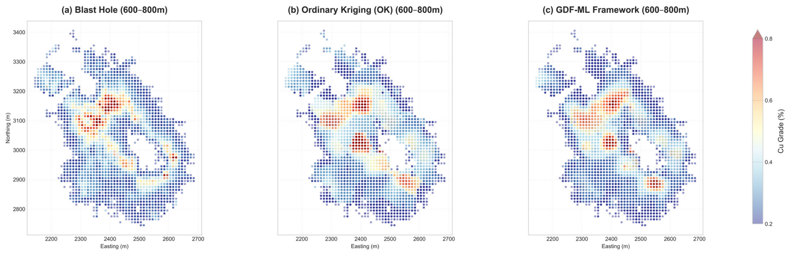
To evaluate the operational stability of the proposed workflow under production conditions, the spatial configurations of the estimated copper grades at the 600–800 m elevation interval are compared directly against the baseline established by high-density blast-hole data. This spatial interval contains the central mineralized system, capturing dense sampling clusters and short-range non-stationary grade transitions that present technical constraints for conventional interpolation routines.

5.6.2. Morphological Fidelity and Spatial Patterns

The spatial distributions of predicted and measured Cu metrics (Figure 11) demonstrate distinct geometric alignment behaviors across the different estimation configurations. The baseline blast-hole data configuration (Figure 11a) characterizes a highly heterogeneous environment with individualized high-grade localization and distinct grade transitions at peripheral margins. The continuous grid generated via Ordinary Kriging (Figure 11b) exhibits characteristically continuous spatial smoothing across the interpolation plane. This mathematical smoothing combines adjacent discrete high-grade pods and extends mineralized energy into sparse or barren peripheral zones, resulting in blurred spatial contacts. In contrast, the expert-constrained regression framework (Figure 11c) accommodates these sharp boundaries and maintains the geometric distinction of the localized grade clusters. By utilizing continuous distance fields as structural constraints rather than hard geometric partitioning, the model reproduces the macroscopic continuity of the mineralization zones while honoring the variance thresholds derived from the high-density production dataset.

5.6.3. Quantitative Analysis of Resource Reliability

The comparative performance metrics indicate a distinct numerical divergence between traditional geostatistical estimation and the proposed GDF-ML framework. At a 0.2% Cu cut-off grade, the Ordinary Kriging (OK) model yields a mean grade of 0.413% (Table 5), representing a positive grade bias of +9.68% relative to the production baseline (0.376%). This deviation reflects a known smoothing effect of linear weighted estimators in high-variance environments. Localized averaging across sharp geological boundaries tends to smear high-grade values into peripheral lower-grade volumes, artificially raising the estimated grade in those zones and resulting in a positive overall bias.
In contrast, the GDF-ML framework achieves a mean grade of 0.379%, reducing the global grade bias to +0.79%. This alignment with the high-density blast-hole data indicates that by embedding GDFs as continuous spatial covariates, the machine learning architecture incorporates the geometric controls of the mineralization system into the regression pathways. Rather than relying on simple spatial proximity averaging, the framework enforces a geometry-conditioned estimation, ensuring that grade values conform to the macro-scale structural context of each block. This consistency demonstrates that GDF-ML functions as an effective spatial regularizer, helping to mitigate localized overestimation variance in high-heterogeneity porphyry systems.

5.6.4. Impacts of Anisotropy on Estimation Bias

The observed estimation variance reflects the operational characteristics of conventional linear interpolation when addressing non-stationary spatial distributions. In this study, although the raw sample assays reached a maximum value of 4.60% Cu, the Ordinary Kriging (OK) configuration exhibited a positive volumetric bias of +9.68%, despite the application of a 2.50% grade capping threshold as a localized technical intervention. This deposit architecture is characterized by multiple mineralization centers, each displaying localized, independent directional anisotropy. Standard linear estimation frameworks typically implement a generalized, globally averaged variogram function, which can smooth out these localized, multi-centered spatial gradients. Consequently, even with the imposition of a 2.50% top-cut threshold, the localized linear weight assignment inherent in the kriging covariance matrix can distribute high-grade energy into peripheral lower-grade domains, occasionally resulting in localized overestimation around these cores.
To mitigate this spatial smoothing effect, conventional geostatistical workflows frequently implement restrictive manual spatial partitioning and empirical data filtering. While these localized geometric interventions modify the localized variance structure, they can alter short-range directional orientations and spatial gradients. In contrast, the expert-constrained regression workflow achieves a closer numerical approximation relative to the high-density production baseline, demonstrating a localized deviation of +0.79% without requiring empirical data clipping or rigid top-cut adjustments. By incorporating continuous distance fields as multi-dimensional covariates, the algorithm accommodates varying localized anisotropy and multiple mineralization centers within an integrated feature space. This continuous configuration allows the higher peak assay metrics to be incorporated while constraining high-grade spatial trends conditional on the interpreted reference boundaries, thereby providing a consistent mathematical approach for long-term resource assessment.

5.7. The Role of Expert Knowledge

The GDF-ML workflow is designed to operate within a knowledge-driven framework, where expert geological interpretation provides the foundational structural constraints. It translates interpreted geological boundaries into machine-readable continuous variables, embedding domain expertise directly into the regression architecture.

5.7.1. Structural Encoding of Geological Expertise

The primary operational objective of this workflow is to convert interpreted spatial boundaries and structural criteria into continuous geometric covariates through the calculation of distance fields. Through this geometric transformation, any given estimation block is evaluated within a continuous spatial framework relative to critical mineralizing controls—such as intrusive margins or structural contacts—rather than as an isolated coordinate point.
In deposit environments characterized by high spatial heterogeneity and pronounced nugget effects, raw sampling datasets incorporate substantial short-range random variance. Delineating the core structural framework provides a geometric baseline for the multi-dimensional feature space, constraining the regression pathways to follow macroscopic spatial trends rather than matching short-range stochastic noise or localized assay anomalies.

5.7.2. Inference and Validation of Structural Frameworks

It is useful to distinguish the expert-constrained regression workflow from deterministic geometric assignment or rigid classification routines. The tree-based ensemble algorithms utilized within this framework perform multi-dimensional non-linear regression conditional on the input covariates. The algorithm evaluates the empirical joint distribution of the training data to optimize the non-linear mapping between the distance fields and the continuous target variables.
This formulation establishes an interactive workflow wherein the geological interpretation defines the geometric constraints and the empirical data dictates the final regression pathways. If a reference boundary or structural interface lacks statistical correspondence with the underlying assay distribution, the resulting variance inflation or performance decay observed during cross-validation provides an empirical diagnostic indicator regarding the spatial consistency of the initial structural model.

5.7.3. Explainable AI (XAI) as a Diagnostic Interface

To interpret the regression model and evaluate the relationship between input features and predictions, we implemented SHAP (SHapley Additive exPlanations) analysis. These metrics quantify the contribution of each geologically derived distance covariate to the block estimates, allowing for a quantitative assessment of how individual features influence the model’s output.
By analyzing these attribution distributions, we can assess whether the model’s internal partitioning aligns with the spatial gradients expected in porphyry systems. This analytical approach allows for a cross-validation between the model’s mathematical output and the underlying geological framework: we evaluate the model’s performance via loss minimization and then verify the consistency of the feature importance metrics with known geological controls. This process ensures that the spatial distribution of the model’s estimates remains consistent with the geological structural context.

5.8. Boundary Conditions and Practical Applicability of the GDF-ML Framework

The application of the GDF-ML framework for grade estimation in heterogeneous porphyry systems depends on specific geological and mathematical constraints. In practice, this workflow functions as a geometry-constrained regression method, not as an unconstrained tool for large-scale spatial prediction. The stability of the model estimates is closely related to how accurately the input distance fields represent the actual geometry. Therefore, the workflow requires a consistent initial interpretation of the main structures—such as mineralized conduits, alteration zones, or lithological contacts—to serve as spatial references. In early-stage exploration, when drill spacing is too wide to build a representative geometric model, the method becomes less useful. Without continuous distance variables, the model cannot properly handle spatial non-stationarity.
When applying the GDF-ML workflow, it is important to distinguish between two different tasks: spatial extrapolation beyond known data, and localized grade characterization within interpreted mineralized zones. The main strength of the GDF-ML method is in evaluating grade trends within a well-defined volume to support long-term mine planning and manage variability. It does this by using continuous distance variables to reduce the excessive smoothing that often affects simpler linear estimators. However, the method is not designed for long-range extrapolation into unsampled areas. Since the model learns from the relationship between structural distance fields and assay values, the absence of data outside the interpreted volume means the algorithm lacks geometric reference. In such cases, estimation variance increases significantly, making the results unreliable.
Furthermore, the GDF-ML workflow integrates qualitative geological knowledge into the optimization process through the selection of primary reference boundaries. While the final block estimates remain conditional on the initial structural interpretations, these geologically defined boundaries function as statistical priors that constrain the multi-dimensional feature space. By incorporating SHAP attribution metrics, the workflow evaluates the marginal contribution of each distance variable to the final partitioning sequences, providing an empirical mechanism to examine whether the selected geometric covariates correspond with the global variance distribution of the target variables. This diagnostic sequence establishes a structured relationship between data-driven optimization and conceptual geological models.
Finally, the regression approach assumes that the calculated distance fields are geometrically continuous. For the model to work effectively, the data used for training and the volume being estimated must share a consistent structural framework. When spatial continuity is broken by post-mineralization faults or complex cross-cutting intrusions, the workflow can still handle these disruptions by adding extra distance fields that specifically represent those boundary features. By treating these structural offsets as distinct numerical inputs rather than as random noise, the regression model preserves mathematical consistency across separate structural blocks. In practical engineering terms, the GDF-ML framework should be seen as an expert-guided estimation method, where its performance limits are set by how well the geological priors can be interpreted and how completely the distance fields capture the relevant structures.

6. Conclusions

This study presents the Geological Distance Field-Machine Learning (GDF-ML) framework as a structured method for addressing spatial non-stationarity and mitigating localized smoothing in porphyry copper grade estimation. By integrating multi-threshold distance features—derived from lithological contacts (NDTI), alteration zones (NDT_Alt), and grade shells (NDTS)—the workflow transforms discrete geological interpretations into continuous numerical variables. This configuration allows ensemble models to characterize complex grade gradients based on empirical variance within the sampling dataset.
Sensitivity testing confirms that the framework’s stability depends on the geometric fidelity of the input structural models. The achieved spatial cross-validation R2 of 0.851 serves as a quantitative indicator of the structured geological information extracted and retained by the model, rather than a measure of deterministic fitting to raw noise. This demonstrates the model’s capacity to resolve non-linear relationships between spatial heterogeneity and multi-source distance metrics.
In a practical application on a porphyry copper deposit in Pakistan, the Random Forest model reduced the mean grade deviation to +0.79% and mitigated the spatial smoothing effects common in conventional Ordinary Kriging workflows. Furthermore, SHAP attribution analysis confirms that the model’s predictive pathways are consistently driven by these geologically derived distance metrics. By automating the parameterization of multi-scale spatial trends, this architecture offers a stable and practical tool for long-term resource characterization and digital mine planning.

Funding

This research received no external funding.

Data Availability Statement

The original data presented in this study are openly available in Zenodo at https://doi.org/10.5281/zenodo.19182803.

Acknowledgments

We thank the anonymous reviewers for their constructive comments.

Conflicts of Interest

Author Liwei Yan was employed by the company MCC Tongsin Resources Ltd. The author declares no conflicts of interest.

Abbreviations

The following abbreviations are used in this manuscript:
GDF-MLGeological Distance Field–Machine Learning
SDFSigned Distance Field

References

  1. Sillitoe, R.H. Porphyry Copper Systems. Econ. Geol. 2010, 105, 3–41. [Google Scholar] [CrossRef]
  2. Afzal, P.; Alghalandis, Y.F.; Khakzad, A.; Moarefvand, P.; Omran, N.R. Delineation of mineralization zones in porphyry Cu deposits by fractal concentration–volume modeling. J. Geochem. Explor. 2011, 108, 220–232. [Google Scholar] [CrossRef]
  3. James, C.; David, R.C.; John, L.W.; Holly, S. Geology, Mineralization, Alteration, and Structural Evolution of the El Teniente Porphyry Cu-Mo Deposit. Econ. Geol. 2005, 100, 979–1003. [Google Scholar] [CrossRef]
  4. Lewis, B.G.; Jorge, Q.G. Patterns of Mineralization and Alteration Below the Porphyry Copper Orebody at El Salvador, Chile. Econ. Geol. 1995, 90, 2–16. [Google Scholar] [CrossRef]
  5. Liu, H.; Wang, Q.; Zhang, C.; Lou, D.; Zhou, Y.; He, Z. Spatial pattern and dynamic control for mineralization in the Pulang porphyry copper deposit, Yunnan, SW China: Perspective from fractal analysis. J. Geochem. Explor. 2016, 164, 42–53. [Google Scholar] [CrossRef]
  6. Cressie, N. Spatial Prediction and Ordinary Kriging. Math. Geol. 1988, 20, 405–421. [Google Scholar] [CrossRef]
  7. Yamamoto, J.K. Correcting the Smoothing Effect of Ordinary Kriging Estimates. Math. Geol. 2005, 37, 69–94. [Google Scholar] [CrossRef]
  8. Emery, X.; Ortiz, J.M. Estimation of Mineral Resources Using Grade Domains: Critical Analysis and a Suggested Methodology. J. South. Afr. Inst. Min. Metall. 2005, 105, 247–256. [Google Scholar]
  9. Maleki, M.; Mery, N.; Soltani-Mohammadi, S.; Plaza-Carvajal, J.; Varouchakis, E.A. Integrating Geological Domains into Machine Learning for Ore Grade Prediction: A Case Study from a Porphyry Copper Deposit. Minerals 2025, 15, 1175. [Google Scholar] [CrossRef]
  10. Hong, J.; Khalil, Y.S.; Narejo, A.A.; Yang, X.; Khan, T.; Wang, Z.; Tang, H.; Zhang, H.; Yang, B.; Li, W. Magmatic Evolution at the Saindak Cu-Au Deposit: Implications for the Formation of Giant Porphyry Deposits. Minerals 2025, 15, 768. [Google Scholar] [CrossRef]
  11. Wang, L.; Zheng, Y.; Hou, Z.; Xue, C.; Yang, Z.; Shen, Y.; Li, X.; Ghaffar, A. The subduction-related Saindak porphyry Cu-Au deposit formed by remelting of a thickened juvenile lower crust underneath the Chagai belt, Pakistan. Ore Geol. Rev. 2022, 149, 105062. [Google Scholar] [CrossRef]
  12. Rose, A.W. Zonal Relations of Wallrock Alteration and Sulfide Distribution at Porphyry Copper Deposits. Econ. Geol. 1970, 65, 920–936. [Google Scholar] [CrossRef]
  13. Sillitoe, R.H. The Tops and Bottoms of Porphyry Copper Deposits. Econ. Geol. 1973, 68, 799–815. [Google Scholar] [CrossRef]
  14. Basson, I.J.; Anthonissen, C.J.; McCall, M.J.; Stoch, B.; Britz, J.; Deacon, J.; Strydom, M.; Cloete, E.; Botha, J.; Bester, M.; et al. Ore-structure relationships at Sishen Mine, Northern Cape, Republic of South Africa, based on fully-constrained implicit 3D modelling. Ore Geol. Rev. 2017, 86, 825–838. [Google Scholar] [CrossRef]
  15. Wang, J.; Zhao, H.; Bi, L.; Wang, L. Implicit 3D Modeling of Ore Body from Geological Boreholes Data Using Hermite Radial Basis Functions. Minerals 2018, 8, 443. [Google Scholar] [CrossRef]
  16. Oleynikova, H.M.; Alexander; Taylor, Z.; Galceran, E.; Nieto, J.; Siegwart, R. Signed Distance Fields: A Natural Representation for Both Mapping and Planning. In Proceedings of the RSS 2016 Workshop: Geometry and Beyond—Representations, Physics, and Scene Understanding for Robotics, Ann Arbor, MI, USA, 19 June 2016. [Google Scholar]
  17. Zhang, J.Y.; Yao, Q.L. Learning Signed Distance Field for Multi-View Surface Reconstruction. In Proceedings of the IEEE/CVF International Conference on Computer Vision (ICCV), Virtually, 11–17 October 2021; pp. 6525–6534. [Google Scholar]
  18. Jeong Joon, P.P.; Florence; Julian, S.; Richard, N.; Steven, L. DeepSDF: Learning Continuous Signed Distance Functions for Shape Representation. In Proceedings of the IEEE/CVF Conference on Computer Vision and Pattern Recognition (CVPR), Long Beach, CA, USA, 16–20 June 2019; pp. 165–174. [Google Scholar]
  19. Rolo, R.M.; Radtke, R.; Costa, J.F.C.L. Signed distance function implicit geologic modeling. REM-Int. Eng. J. 2017, 70, 221–229. [Google Scholar] [CrossRef]
  20. Leo, B. Random Forests. Mach. Learn. 2001, 45, 5–32. [Google Scholar]
  21. Chen, T.; Guestrin, C. XGBoost. In Proceedings of the 22nd ACM SIGKDD International Conference on Knowledge Discovery and Data Mining, San Francisco, CA, USA, 13–17 August 2016; pp. 785–794. [Google Scholar]
  22. Zhang, P.; Jia, Y.; Shang, Y. Research and application of XGBoost in imbalanced data. Int. J. Distrib. Sens. Netw. 2022, 18, 15501329221106935. [Google Scholar] [CrossRef]
  23. Liudmila, P.; Gleb, G.; Aleksandr, V.; Anna Veronika, D.; Andrey, G. CatBoost: Unbiased boosting with categorical features. In Proceedings of the 32nd Conference on Neural Information Processing Systems (NeurIPS 2018), Montréal, QC, Canada, 2–8 December 2018. [Google Scholar]
  24. Rodríguez, P.; Bautista, M.A.; Gonzàlez, J.; Escalera, S. Beyond one-hot encoding: Lower dimensional target embedding. Image Vis. Comput. 2018, 75, 21–31. [Google Scholar] [CrossRef]
  25. Akiba, T.; Sano, S.; Yanase, T.; Ohta, T.; Koyama, M. Optuna. In Proceedings of the 25th ACM SIGKDD International Conference on Knowledge Discovery & Data Mining, Anchorage, AK, USA, 4–8 August 2019; pp. 2623–2631. [Google Scholar]
  26. Watanabe, S. Tree-Structured Parzen Estimator: Understanding Its Algorithm Components and Their Roles for Better Empirical Performance. arXiv 2023, arXiv:2304.11127. [Google Scholar] [CrossRef]
  27. Eyal, W. The Shapley Value. In Handbook of Garne Theory, Volume 3; North-Holland: Amsterdam, The Netherlands, 2002; pp. 2027–2054. [Google Scholar]
  28. Zhang, M.; Wang, X.; Chen, C.; Ding, J.; Zhou, X.; Qu, J. Interpretable ore classification using SHAP-enhanced LightGBM: A case study from the Qiaomaishan deposit, China. Appl. Comput. Geosci. 2025, 28, 100295. [Google Scholar] [CrossRef]
  29. Chen, Y.; Chen, B.; Shayilan, A. Combining categorical boosting and Shapley additive explanations for building an interpretable ensemble classifier for identifying mineralization-related geochemical anomalies. Ore Geol. Rev. 2024, 173, 106263. [Google Scholar] [CrossRef]
  30. Jairo, M.-A.; Marco, C.-T.; Jose, M.-Q.; Eduardo, N.-V.; Juan, V.-G.; Juan, C.-G. Copper Ore Grade Prediction using Machine Learing Techniques in a Copper Deposit. J. Min. Environ. 2024, 15, 1011–1027. [Google Scholar] [CrossRef]
  31. Jafrasteh, B.; Fathianpour, N.; Suárez, A. Comparison of machine learning methods for copper ore grade estimation. Comput. Geosci. 2018, 22, 1371–1388. [Google Scholar] [CrossRef]
  32. Kaplan, U.E.; Dagasan, Y.; Topal, E. Mineral grade estimation using gradient boosting regression trees. Int. J. Min. Reclam. Environ. 2021, 35, 728–742. [Google Scholar] [CrossRef]
  33. Kaplan, U.E.; Topal, E. A New Ore Grade Estimation Using Combine Machine Learning Algorithms. Minerals 2020, 10, 847. [Google Scholar] [CrossRef]
  34. Maniteja, M.; Samanta, G.; Gebretsadik, A.; Tsae, N.B.; Rai, S.S.; Fissha, Y.; Okada, N.; Kawamura, Y. Advancing Iron Ore Grade Estimation: A Comparative Study of Machine Learning and Ordinary Kriging. Minerals 2025, 15, 131. [Google Scholar] [CrossRef]
Figure 1. Spatial distribution of drill-hole data and Copper (Cu) grades within the study area. (a) 3D perspective view showing the orientation and depth of the drill-holes. (b) Top-down plan view illustrating the spatial coverage across Easting and Northing coordinates. The color scale indicates the Cu grade (wt.%), highlighting the high-grade mineralization zones (red) concentrated in the central portion of the drilling campaign.
Minerals 16 00573 g001
Figure 2. Schematic workflow of the GDF-ML framework. This methodology integrates structural and alteration models to derive spatial features via cKDTree-based distance calculation, followed by ensemble learning (RF, XGBoost, CatBoost) and SHAP-based geological consistency auditing, ultimately enabling the estimation of grade distributions across the 3D block model in accordance with geological constraints.
Minerals 16 00573 g002
Figure 3. Illustration of the Geological Distance Field (GDF) derived from an interpreted structural interface. The central yellow ring represents a discrete geological reference (e.g., an iso-grade shell or intrusive contact). The continuous scalar field represents the GDF, where color gradients quantify the spatial affinity to the mineralizing core. Negative values (blue) denote the proximal environment within the structural boundary, while positive values (red) characterize the distal peripheral environment. This field serves as a physicochemical proxy, transforming absolute spatial coordinates into a theory-consistent geological coordinate system.
Minerals 16 00573 g003
Figure 4. Implicitly reconstructed 3D macro-architecture of the porphyry system. (ah) Progressive visualization of grade shells ranging from 0.1% to 1.5% Cu, serving as multi-scale geometric constraints for mineralized intensity. (ik) Representative alteration domains, including potassic, propylitic, and sericite zones, which provide hydrothermal zonation logic for the model. (l) The Tonalite intrusive body, functioning as the primary lithological skeleton.
Minerals 16 00573 g004
Figure 5. Scatter plot of measured vs. predicted copper grades for the 20% independent test set under structural perturbation. The plot illustrates the model’s predictive performance when 20% of the samples are withheld from the Geological Distance Field (GDF) construction. The resulting R2 of 0.6559 and MAE of 0.0928 reflect the sensitivity of the GDF-ML framework to local geometric variations in the underlying geological constraints. The color scale represents the absolute error (residuals), highlighting that while the global structure remains robust, subtle perturbations in the GDF near withheld points lead to a decline in local estimation precision compared to the primary models.
Minerals 16 00573 g005
Figure 6. The feature importance ranking, based on mean absolute SHAP values, quantifies the average impact magnitude of each variable on copper grade estimation and highlights the hierarchical contribution of various geological constraints. Grade Shell (NDTS) features, particularly NDTS05, emerge as the dominant drivers of the model’s decision-making, indicating that the system relies most heavily on expert-defined mineralization boundaries to inform its output. In contrast, lithological (NDTI) and alteration features exhibit lower but consistent importance, serving as secondary spatial constraints that refine the model’s understanding of the deposit architecture alongside the primary grade shell constraints.
Minerals 16 00573 g006
Figure 7. The SHAP beeswarm plot reveals a distinct long-tailed distribution along the positive axis for key Grade Shell features (NDTS). The extended tails of blue dots (low distance values) signify that samples located within close proximity to the expert-defined grade shells receive a higher positive predictive contribution within the regression pathways. This numerical distribution confirms that the trained model’s decision pathways selectively allocate higher predictive importance to these localized geometric zones based strictly on the variance constraints of the input database.
Minerals 16 00573 g007
Figure 8. SHAP dependence analysis showing the non-linear response of the model to diverse structural distance metrics: (a) NDTS05; (b) NDTS02; (c) NDTS03; (d) NDTS06; (e) NDTS10; (f) NDTS01; (g) NDTS08; (h) NDTS15; (i) NDTI; (j) NDT_Alt_Potassic; (k) NDT_Alt_Sericite; and (l) NDT_Alt_Propylitic. The scatter plots are color-coded by measured copper grades, revealing a systematic alignment between the model’s predictive contributions (SHAP values) and the actual mineralization trends. The threshold-like transitions near the geometric zero-planes (x ≈ 0) across these structural features confirm that the model systematically utilizes these hierarchical geological constraints to regulate estimation paths and effectively map non-linear spatial mineralization gradients. The red dashed line represents the geometric zero-plane of the corresponding geological features.
Minerals 16 00573 g008
Figure 9. SHAP waterfall plot of a representative sample (Actual Cu: 0.400). This plot documents the localized predictive adjustments from the baseline E[f(X)] = 0.291 to the final output f(x) = 0.394. The positive estimation shifts are driven by the 0.2% and 0.3% grade shells (NDTS02 and NDTS03), while the position outside the 0.5% grade shell (NDTS05) triggers a negative adjustment of −0.05, confirming that these geometric features directly guide the model’s localized estimation pathways.
Minerals 16 00573 g009
Figure 10. 3D block model and spatial distribution of copper grades. (a) 3D view of the estimated block model at a 0.2% Cu cut-off grade. (b) Visualization of the high-grade core (>0.35% Cu), showing the localized spatial configuration of high-grade zones within the block framework. (c) Global plan view projected across Easting and Northing coordinates. (d) Horizontal level slice (700–750 m elevation) revealing the internal grade continuity. The color bar indicates the copper grade (wt.%), ranging from low (blue) to high (red).
Minerals 16 00573 g010
Figure 11. Visual comparison of Cu grade spatial patterns at the 600–800 m elevation. (a) Production Data: High-density blast-hole samples illustrating the reference distribution, characterized by discrete high-grade clusters and well-defined mineralization boundaries. (b) Ordinary Kriging (OK): The resulting estimate exhibits pronounced spatial oversmoothing, resulting in a reduction in local variance where distinct high-grade zones are integrated into broader, continuous areas. (c) GDF-ML Framework: The predicted distribution shows high morphological fidelity to the production data, preserving cluster independence and honoring sharp geological transitions without the requirement for manual domaining.
Minerals 16 00573 g011
Table 1. Regression Performance Metrics and Optuna Optimization Results for 5-fold validation for Shuffled Data.
ModelR2_5-Fold CVFull_Data_R2Best_Params
Random Forest0.868 0.940n_estimators: 729, max_depth: 17, min_samples_leaf: 5
CatBoost0.849 0.913iterations: 1178, depth: 4, learning_rate: 0.0197
XGBoost0.854 0.916 n_estimators: 1500, max_depth: 3, learning_rate: 0.0101, subsample: 0.688
Table 2. Regression Performance Metrics and Optuna Optimization Results for 2-fold validation for Shuffled Data.
ModelR2_2-Fold CVFull_Data_R2Best_Params
Random Forest0.872 0.940n_estimators: 489, max_depth: 13, min_samples_leaf: 4
CatBoost0.846 0.905iterations: 743, depth: 4, learning_rate: 0.0229
XGBoost0.844 0.932 n_estimators: 1040, max_depth: 4, learning_rate: 0.0132, subsample: 0.679
Table 3. Regression Performance Metrics and Optuna Optimization Results for 2-fold Validation for Non-shuffled Data.
ModelR2_2-Fold CVFull_Data_R2Best_Params
Random Forest0.867 0.918n_estimators: 512, max_depth: 8, min_samples_leaf: 4
CatBoost0.841 0.945iterations: 968, depth: 7, learning_rate: 0.0323
XGBoost0.838 0.915 n_estimators: 518, max_depth: 8, learning_rate: 0.0287, subsample: 0.800
Table 4. Regression Performance Metrics and Optuna Optimization Results for Spatial Validation Test.
ModelR2_2-Fold CVFull_Data_R2Best_Params
Random Forest0.851 0.925n_estimators: 994, max_depth: 10, min_samples_leaf: 5
CatBoost0.788 0.966iterations: 998, depth: 9, learning_rate: 0.0428
XGBoost0.819 0.906 n_estimators:880, max_depth: 3, learning_rate: 0.0114, subsample: 0.802
Table 5. Comparative performance of resource estimation models (600–900 m elevation).
Model TypeMean Grade (Cu %)Tonnage (t)Grade Bias (vs. Actual)
blast-hole0.37670,475,600
Ordinary Kriging (OK)0.41372,922,200+9.68%
GDF-ML Framework0.37973,265,400+0.79%
Disclaimer/Publisher’s Note: The statements, opinions and data contained in all publications are solely those of the individual author(s) and contributor(s) and not of MDPI and/or the editor(s). MDPI and/or the editor(s) disclaim responsibility for any injury to people or property resulting from any ideas, methods, instructions or products referred to in the content.