Article

Reconstructing Depositional Environments with Decision Tree Classifier (A Machine Learning Model): A Grain-Size Study of the Tredian Formation, Salt Range, Pakistan

1
Department of Earth Sciences, Quaid-i-Azam University, Islamabad 45320, Pakistan
2
Department of Geology, University of Vienna, 1090 Vienna, Austria
3
Department of Geology and Mines, Faculty of Science, Nangarhar University, Jalalabad 3801, Afghanistan
4
Department of Software Engineering, University of Malakand, Chakdara 18800, Pakistan
5
Department of Geology, University of Swabi, Swabi 23562, Pakistan
*
Authors to whom correspondence should be addressed.
Minerals 2026, 16(5), 512; https://doi.org/10.3390/min16050512
Submission received: 23 March 2026 / Revised: 23 April 2026 / Accepted: 27 April 2026 / Published: 13 May 2026
(This article belongs to the Section Mineral Exploration Methods and Applications)

Abstract

The Middle Triassic Tredian Formation of the Salt Range, Pakistan, consists of sandstones with interbedded shale in the lower part and minor dolomite in the upper part. Conventional grain-size analysis has been widely used as a sedimentological tool to elucidate depositional environments and the mode of transportation of detrital sediments. This study presents the first integrated application of a Decision Tree Classifier (a machine learning model) with field and petrographic evidence to interpret grain-size statistics for the analysis of depositional environments of the Tredian Formation in the Salt Range, Pakistan. Stratigraphic sections of the Tredian Formation were measured and sampled in the Nammal Gorge and Zaluch Nala in the Salt Range for detailed sedimentological and grain-size analyses. The lower part of the Tredian Formation (Landa Member) consists of interbedded sandstone and shale (LF-1) characterized by large-scale slumps, parallel lamination, ripple marks, and cross-bedding. The LF-1 is overlain by the Katkhiara Member, which is dominated by thick sandstone (LF-2) with planar and trough cross-bedding and contains dolomite beds (LF-3) in the upper part. Grain-size statistics show that the sandstones are fine-to-medium-grained, well-to-very-well-sorted, near-symmetrical, and very platykurtic. Machine learning-based bivariate plots suggest that most of the samples are grouped, with some showing scattered trends. The Linear Discriminant Function (LDF) analysis indicates that the Tredian Formation was deposited in fluvial–deltaic to shallow marine environments with sand reworking and redistribution under aeolian/beach settings. The Decision Tree Classifier Model (DTCM) predicted fluvial to shallow marine depositional environments for the Tredian Formation and shows strong agreement with field-based lithofacies interpretation, demonstrating its reliability as a predictive tool. Thus, the present study demonstrates that integrating grain-size-based machine learning and statistical analysis with traditional sedimentology provides valuable insights into depositional settings and enhances the reliability of interpretations of ancient sedimentary environments.

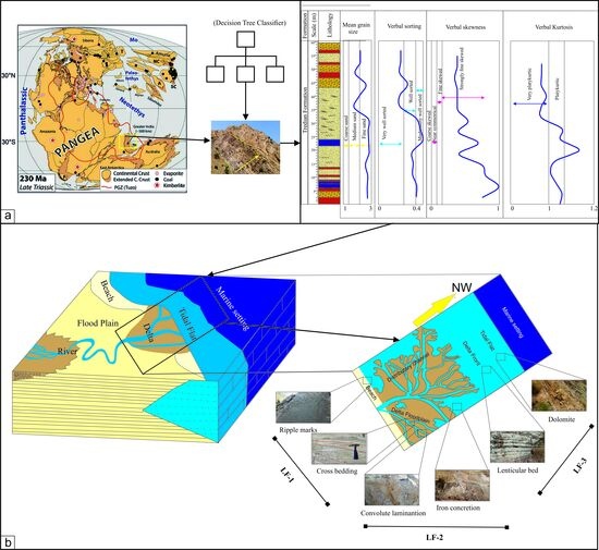
Graphical Abstract

1. Introduction

In the recent past, the use of machine learning (ML) has gained popularity among geoscientists. Some of the fields in which ML techniques have been successfully utilized in the geosciences industry include lithofacies identification, reservoir characterization and prediction, and various reservoir portfolio management [1,2,3,4,5,6]. The technique is becoming increasingly popular due to its ability to analyze complex datasets and make reliable predictions.
Grain size is the basic feature of sediments and is one of the most important descriptive properties of siliciclastic rocks. Grain-size analysis and its characteristics are widely used to decode depositional patterns, processes, depositional environments, and hydrodynamic conditions [7]. In addition, it also provides information about transportation mechanisms and depositional conditions [8,9]. However, traditional methods of grain-size analysis, such as cumulative curves and bivariate and statistical parameters, have many applications, but these are often subjective and may lose important non-linear relationships within the data [7,8,9,10,11]. Manual as well as graphical techniques can be tedious and time-consuming, especially for large datasets, because they are not reproducible. This shows the need for more objective and pattern-recognition, data-driven methods that can enhance the reliability of depositional environment classification [10,11,12].
The utility of ML techniques in grain-size analysis is one of the alternative methods for extensive calculations. Traditional methods of grain-size calculation are based on statistical regressions and empirical equations. Depositional units, lateral and vertical patterns, and associated variables such as grain size, porosity, or permeability within the core samples can be identified by using Self-Organizing Maps (SOMs), which are a type of artificial neural network that uses a structure of self-adapted elements [10,11]. ML has been used in provenance analysis (i.e., point counting and grain identification) [12]. ML models (i.e., Unsupervised Vector Quantizer Artificial Neural Network (UVQ–ANN) and Sequential Indicator Simulation (SIS)) are used to delineate subsurface rock units by developing a facies model to study depositional processes and facies distributions [13]. Therefore, the use of modern tools, including ML and Alternative Intelligence (AI) models, in addition to traditional grain-size statistics, provides an integrated approach for sedimentological interpretations [10,11,12,13].
This study integrates outcrop-based lithofacies analysis and the depositional environment interpretation with a machine learning-driven model to evaluate grain-size statistical parameters, petrographic characteristics, and the overall depositional framework of the Tredian Formation exposed in the geologically renowned Salt Range of Pakistan. This will help to reconstruct an integrated approach for lithofacies analysis and depositional environmental interpretation and evaluate the reliability of the use of the ML-based Decision Tree Classifier Model (DTCM) as a tool to predict depositional settings.
This study provides a more robust approach toward depositional environmental interpretation, in addition to chronophagous and irreproducible traditional petrographic studies, without losing reliable field information. Field-based sedimentological data and petrographic data were used in traditional depositional interpretation. Petrographic data, including point-counting and grain-size parameters, were used as input parameters for the DTCM, and the interpretation was validated against the lateral and vertical facies variation and sedimentary structures observed in the field.

2. General Geology and Stratigraphy

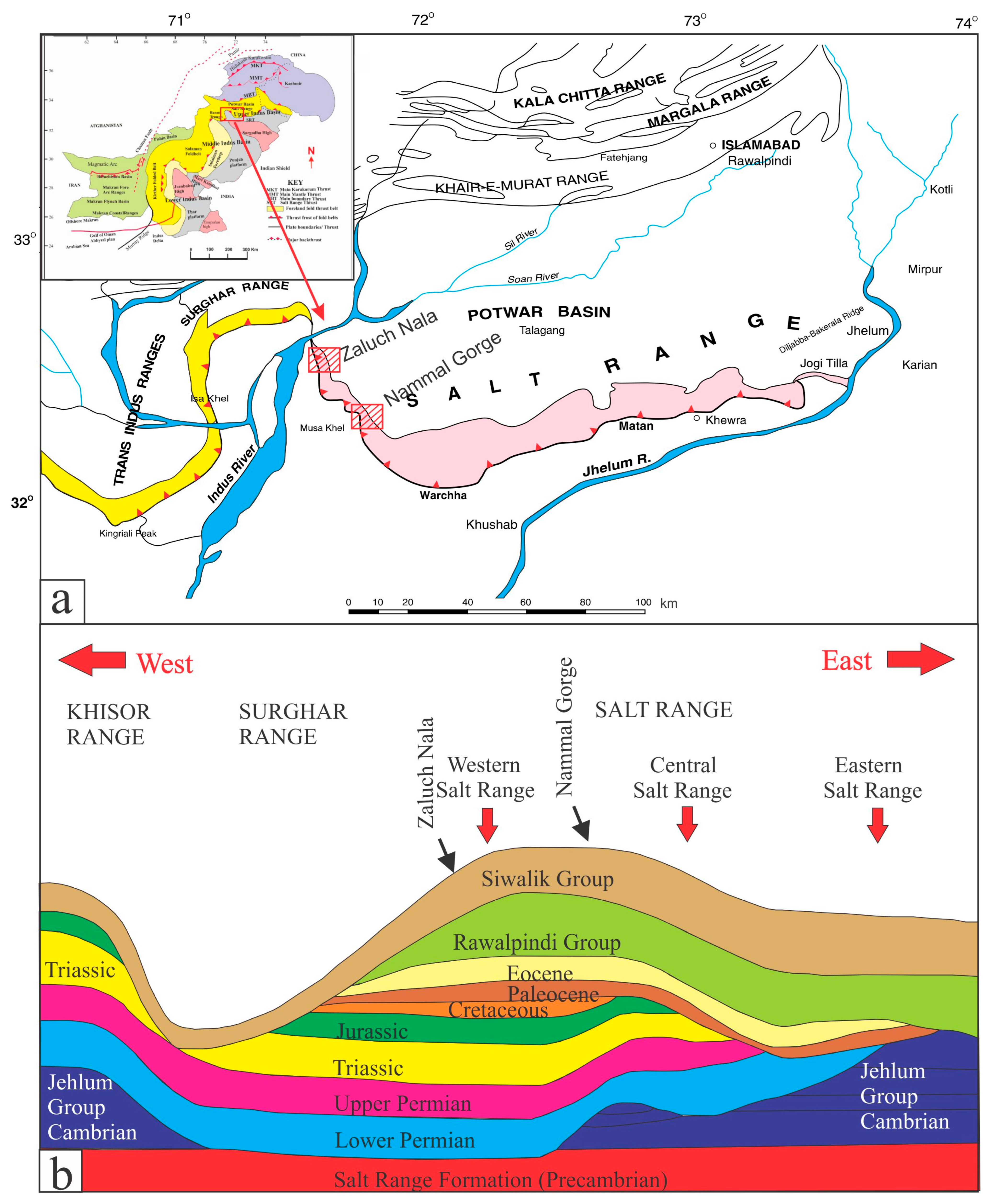
The Salt Range is located in the southern part of the foreland zone of the Himalayan Fold and Thrust Belt (HFTB) and marks the southern boundary of the Potwar Plateau (Figure 1). It formed as a result of the Himalayan Orogeny, and the Precambrian evaporites of the Salt Range Formation play a key role in controlling the surface structural geometries [14,15]. The Salt Range Thrust (SRT) is the main decollement in this compressional regime, and the Salt Range is its surface expression, where Precambrian to Pliocene strata have been thrusted over the Pleistocene molasses of the Indo-Gangetic Plain [15,16,17,18].
The Late Permian–Early Triassic time was characterized by global climate change and complex paleogeography [19] with the supercontinent Pangaea surrounded by the Panthalassa Ocean [20]. In the Salt Range, a monsoon-like climate with summer and winter circulation was prevalent in the Early Triassic, despite an overall warm and temperate climate [21]. The Triassic sedimentation in the Salt Range occurred south of the Neo-Tethyan rift zone [19,22,23,24]. The Triassic stratigraphy of the Salt Range comprises the Mianwali, Tredian and Kingriali formations, collectively called the Musa Khel Group [25].
The Triassic succession has excellent exposures in the western Salt Range, Surghar Range, and Khisor Range (e.g., Nammal Gorge, Zaluch Nala, Vanjari, Paniala, Saiyidwali and Tapan Wahan) [24,26]. The lower contact of the succession is with the Permian Chhidru Formation, marking the Permian–Triassic boundary [19,27], while the upper contact marks the Triassic–Jurassic boundary in the area [28]. The Mianwali Formation is the oldest Triassic unit of the Salt Range, which contains shallow marine sandstones, siltstones, shales, and fossiliferous carbonates. The middle Triassic Tredian Formation conformably overlies the Mianwali Formation and is divided into two members (i.e., Landa Member and Khatkiara Member). The Kingriali Formation conformably overlies the Tredian Formation, is the youngest Triassic unit in the area and contains thick dolomites [29].

3. Materials and Methods

3.1. Fieldwork

The Tredian Formation was measured and sampled at the Zaluch Nala (Lat. 32°39′29″ N and Long. 71°47′52″ E) and the Nammal Gorge (Lat. 32°40′39″ N and Long. 71°47′06″ E) sections of the western Salt Range (Figure 1 and Figure 2). Sedimentological analysis was conducted in the field, bedding behavior and sedimentary structures and features were noted and measured, and photographs were taken where needed (Figure 3, Figure 4 and Figure 5). Both sections were sampled on a variation basis (i.e., lithologies, grain size, and color). Representative samples (total number of samples = 92), including 42 from the Zaluch Nala and 50 from the Nammal Gorge, were collected.

3.2. Paleoflow

To find the paleoflow direction from the cross-stratifications, the long axes of the cross beds and the dip direction of the foresets were measured. Each cross-bed set was measured in the field to get the position of the cross beds and the position of the surfaces bounding the cross beds. A Silva compass (HANZA Group, Suzhou, China) was used to record dip direction and dip amount. The paleocurrent direction was determined by projecting the dip direction of the foresets and the dip direction of the cross beds, since the cross beds are assumed to migrate in the direction of the main current [30]. Directional data are transformed into azimuths and plotted in a rose diagram by using GeoRose (Version 0.5.1) software to show the frequency and pattern of the paleoflow directions within a dataset.
Figure 1. Generalized geological map and cross-sectional view of the Salt and Trans-Indus Ranges. (a) Geological map of the Salt Range: the red boxes mark the studied locations (Nammal Gorge and Zaluch Nala), the pink color indicates the Salt Range, and the yellow color indicates the Trans-Indus ranges [31]. The inset map shows the location of the Salt Range. (b) Generalized lithostratigraphic cross-section of the Salt and Trans-Indus Ranges [23].
Minerals 16 00512 g001
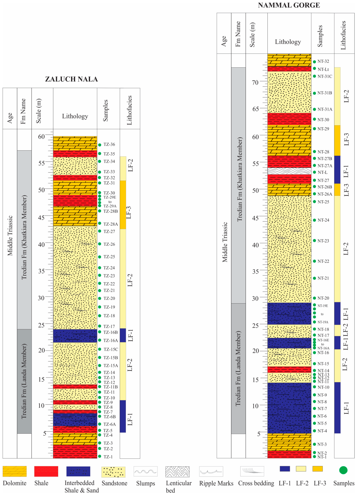
Figure 2. Stratigraphic logs of the Tredian Formation exposed in the Zaluch Nala and the Namal Gorge sections. Sedimentary structures, sample positions, and lithofacies are included. LF-1 (sandstone interbedded with shale lithofacies), LF-2 (thick-bedded sandstone lithofacies) and LF-3 (dolomite lithofacies).
Minerals 16 00512 g002
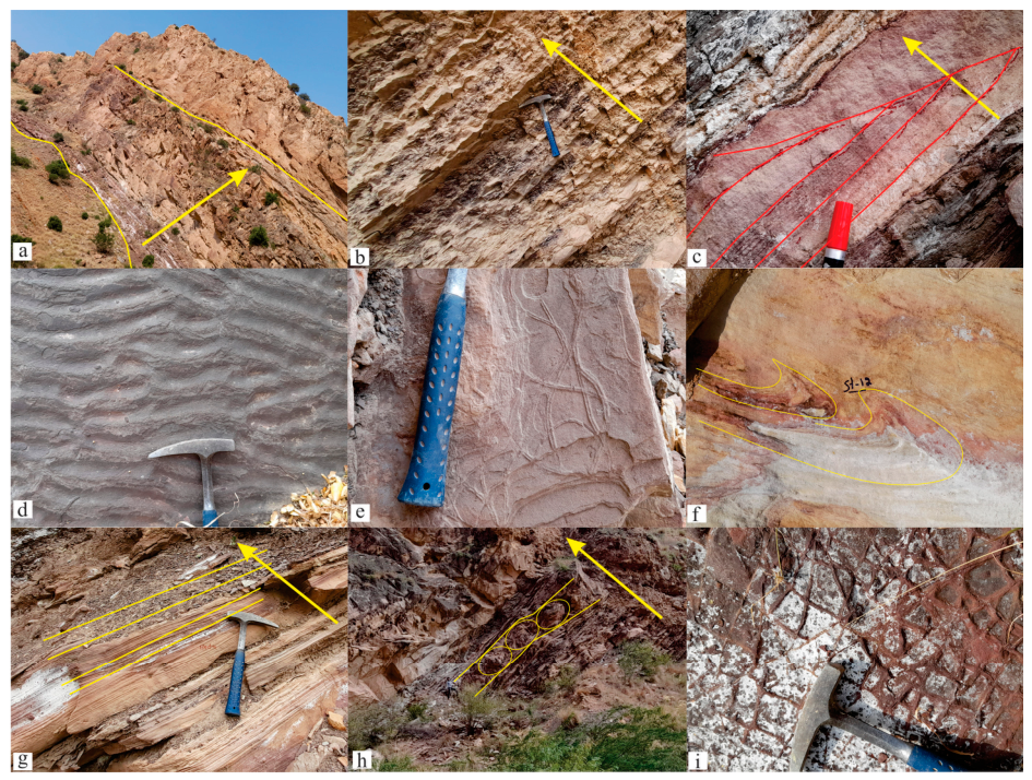
Figure 3. (a) Lower and upper contacts (yellow lines) of the Tredian Formation, arrowhead shows the top; (b) interbedded sandstone and shale, yellow arrow marks the top (LF-1); (c) planar cross-bedded sandstone marked (red lines), yellow arrow marks the top (LF-1); (d) asymmetrical ripple marks (LF-1); (e) Cruziana trace fossil (LF-1); (f) soft-sediment deformation (yellow lines and circles) (LF-1); (g) parallel lamination (yellow lines) (LF-1); (h) slumps in LF-1 (yellow lines); (i) mud cracks.
Minerals 16 00512 g003
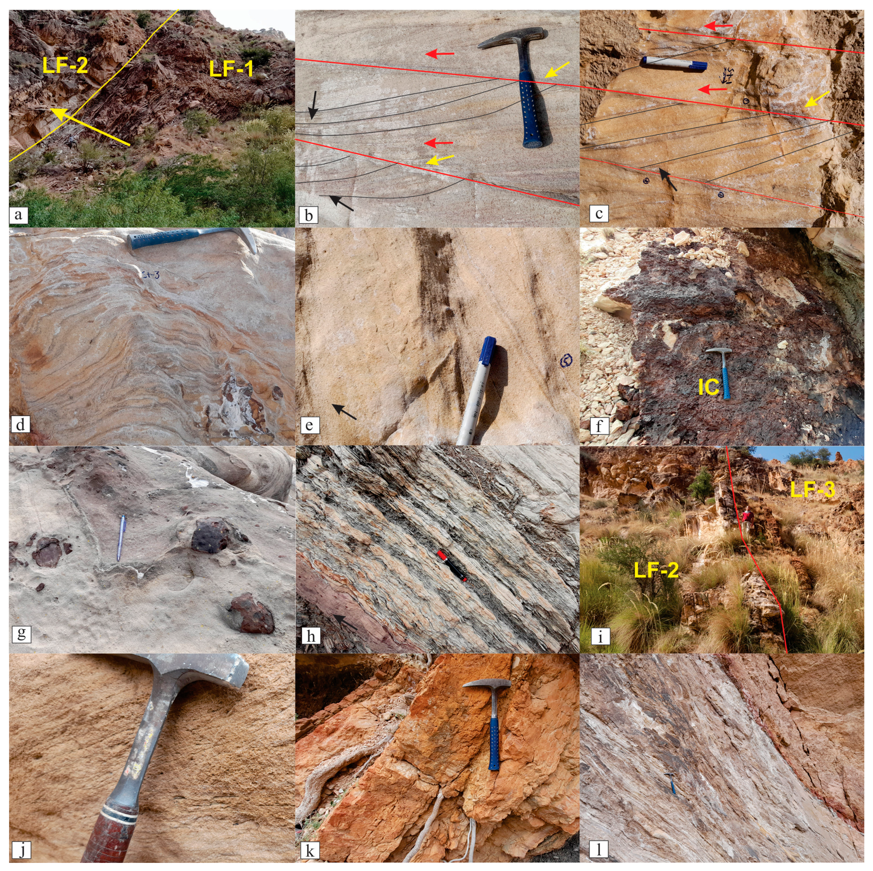
Figure 4. (a) Contact between LF-1 and LF-2 (yellow line) (Nammal Gorge); (b,c) Cross bedded sandstone (red arrow for flow direction, red line for bounding surfaces, yellow arrow for truncated side, black arrow for tangential side) (LF-2); (d) cross-bedded sandstone (LF-2); (e) thick-bedded sandstone (LF-2); (f,g) iron concretion (IC) (LF-2); (h) lenticular bed; (i) contact between LF-2 and LF-3 (yellow line) (Zaluch Nala); (j) sandy dolomite bed; (k) pure dolomite bed in the LF-3 (Nammal Gorge); (l) contact between Tredian Formation and Kingriali Formation (Nammal Gorge).
Minerals 16 00512 g004
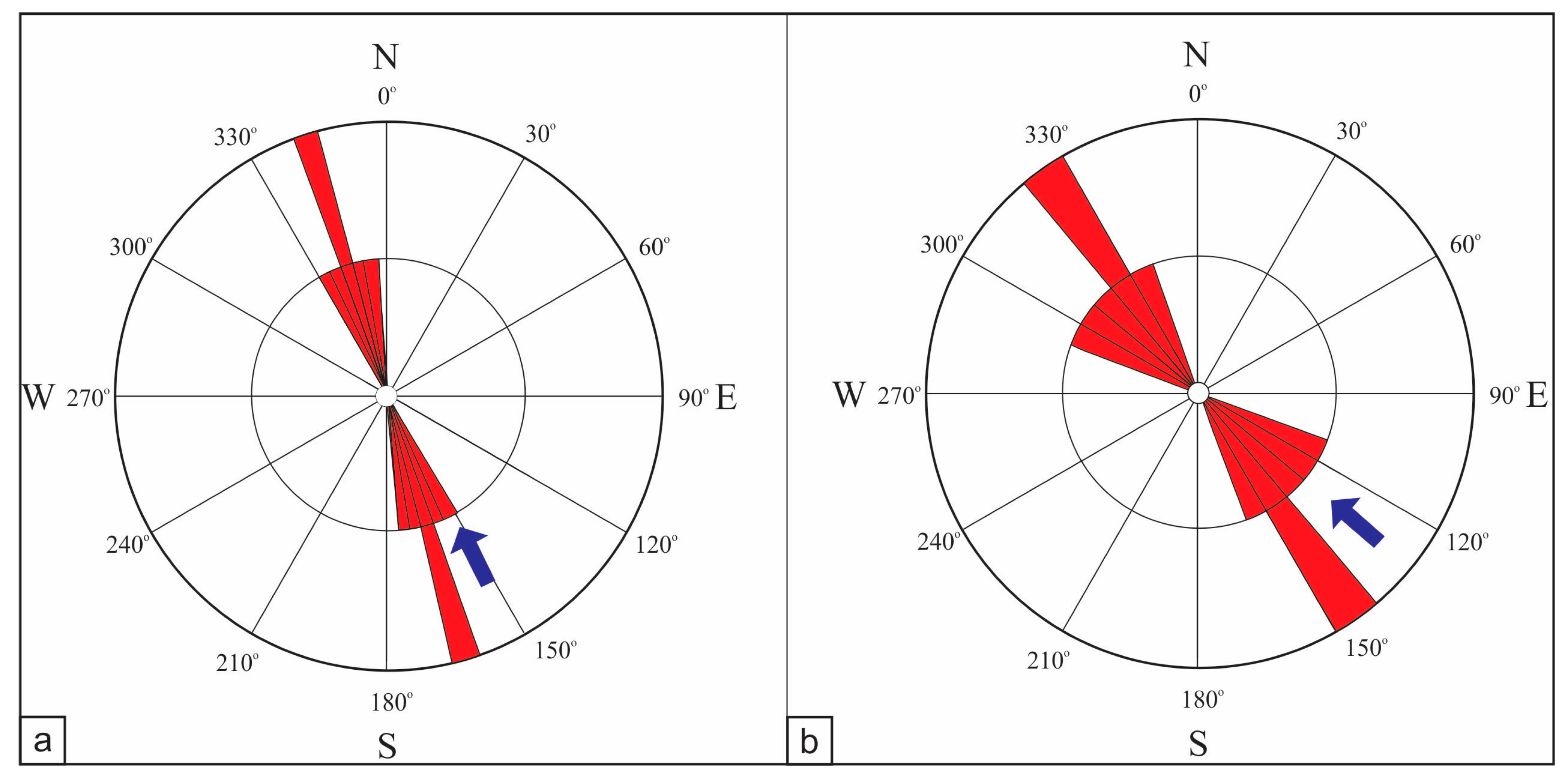
Figure 5. Paleocurrent directions of the Tredian Formation: (a) Zaluch Nala; (b) Nammal Gorge. The paleocurrents indicate a SE to NW paleoflow direction.
Minerals 16 00512 g005

3.3. Lithological Logs

Based on field data, lithological logs were prepared for both sections using CorelDraw2020 software (Figure 2). Lithologies, sedimentary structures and features were marked on these logs to understand the vertical lithological variation and identification of the various lithofacies. The lithological logs were prepared on the same scale (1 cm = 2.5 m) to have an idea of lateral thickness and lithological/lithofacies variations.

3.4. Petrography and Grain Parameters

In total, 48 thin sections, including 23 from Zaluch Nala and 25 from the Nammal Gorge, were prepared from sandstone and carbonates of the Tredian Formation at the Geological Survey of Pakistan (GSP) and Bacha Khan University, Charsadda (BKUC), Pakistan. The thin sections were examined systematically under a polarizing Olympus CX31 microscope (Olympus Corporation, Tokyo, Japan) equipped with a DP-21 camera (Olympus Corporation, Tokyo, Japan) at the Department of Earth Sciences, Quaid-i-Azam University, Islamabad, Pakistan, and photographed at the National Centre of Excellence in Geology (NCEG), Peshawar University, Pakistan, using a Leica DM2700 P microscope with a Leica MC170 HD camera (Leica Microsystems, Wetzlar, Germany).
Petrographic studies focused on framework mineralogical identification, point counting, grain size, and cement and matrix identification (Figure 6, Table 1). Of the total 48 samples, 30 were selected for point counting (including 16 samples from the Nammal Gorge and 14 samples from Zaluch Nala).
The conventional method [32,33,34] was used to measure the grain’s longest axis. In total 500 grains were measured per thin section. The frequency of grain size was calculated by using the Udden–Wentworth grade scale [35,36]. The collected grain-size (mm) data were converted into Phi (Ø) scale by using the following equation:
Ø = −log2D
where Ø is the phi size and D is the grain diameter in millimeters (mm).
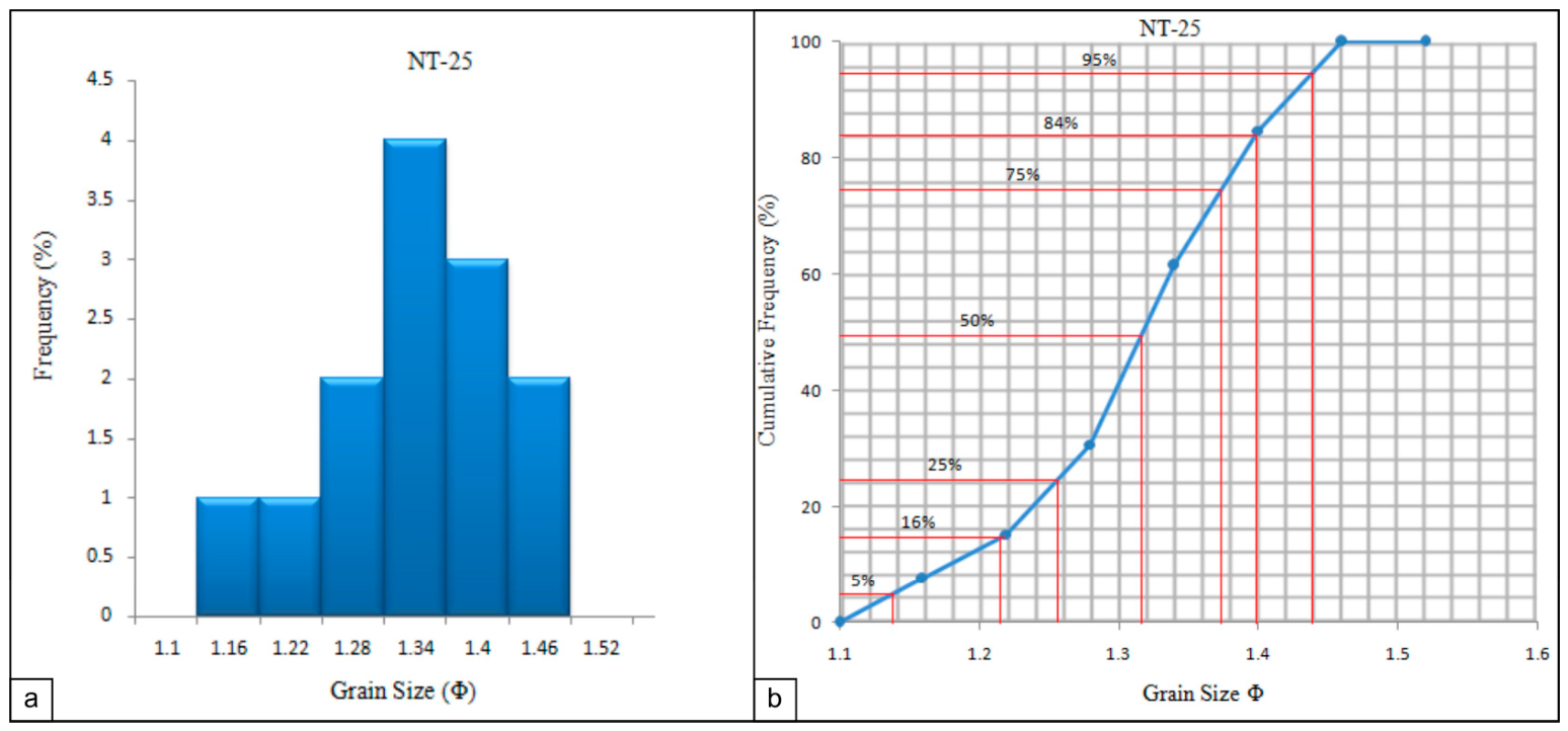
The grain-size data were graphically represented in the form of cumulative curves (Figure 7). However, the determination of the average grain size and grain sorting using manual methods is not reliable [33]. Therefore, mathematical methods were derived from the cumulative curves (Figure 7) to mathematically describe the grain-size distributions, enabling statistical treatment of the grain-size data acquired in petrography [37]. The proposed equation of [38] for the grain-size statistical parameters was used (Table 2). Bivariate scatter plots were utilized to differentiate depositional environments by analyzing the textural differences in sediments. The Linear Discriminant Function (LDF) [39] was used to interpret depositional environments and depositional processes. Four main parameters, including mean, standard deviation, skewness, and kurtosis (source code for all the key parameters and plots can be found in Supplementary Materials), were used to describe grain-size distribution (Table 2). Mean size (Mz) measures the arithmetic average size of all the grains (counted) in the sample. An estimate of the arithmetic mean was calculated by selecting specific percentile values from the cumulative curve and then averaging these values using the graphical mean formula (Table 2). For sorting (σi), the mathematical expression is inclusive graphic standard deviation. The descriptive terms in language correspond to the values of the inclusive graphic phi standard deviation (Table 3), which represents sorting [40].
The degree of symmetry of the grain-size distribution is known as skewness (Ski), or it reflects sorting in the tail of the distribution [8]. Furthermore, it serves as a descriptive parameter that characterizes the bulk of the grain-size measurements, including the graphic skewness. Skewness is indicated by how much the calculated skewness values deviate from zero, with greater deviations indicating a higher degree of skewness (Table 4). The graphic kurtosis (Kz) represents the sharpness of the grain-size frequency curve that compares the sorting or spreading of the middle distribution section to the tail spread (Table 5).

3.5. Machine Learning Model

In ML, the first step is to find the appropriate mathematical model that predicts the quantity or the group of interest. Predicting the continuous values, which is relevant to the present study, is often referred to as regression, and predicting the group is referred to as classification or clustering in machine learning [41]. For the present work, the DTCM was trained, based on the existing inclusive graphical calculated grain-size parameters of [38]. The analysis was done using Anaconda (version 2020.07) software and the Python (version 3.2020) programming language. First, the grain sizes were measured using ImageJ (version 1.x) software.
The dataset was created in Microsoft Excel (.xlsx) format and then converted into Comma-Separated Values (.csv) format to maintain compatibility with Python data analysis. The .csv file was imported into the Anaconda environment, where it was used to develop the DTCM with Python libraries. Some of the libraries used are NumPy (version 2.4.4) for numerical operations, Pandas (version 3.0.2) for organizing and processing data, and Matplotlib (version 3.10.9) for data visualization. The DTCM was implemented and trained using scikit-learn (version 1.8.0). These are strong tools for data analysis, model building and visualization.
The DTCM was chosen primarily for its interpretability and its ability to generate explicit decision rules that can be directly related to sedimentological processes and grain-size characteristics [12]. Unlike more complex models such as Random Forest, Support Vector Machines, and Neural Networks, which often function as “black-box” models, the DTCM provides transparent and easily understandable classifications. Additionally, it effectively captures non-linear relationships within the data without requiring extensive parameter tuning. These features make it particularly suitable for integrating ML results with field-based geological interpretations in the present study.
For model development, the dataset was split into subsets of training and testing with an 80/20 ratio. In this model, the DTCM was trained using 80% of the data, reserving the other 20% for testing. The testing dataset contains the unseen data, which was utilized to assess the predictive accuracy of the model. The data was split using a random state for reproducibility of results.
The evaluation of the DTCM was assessed using standard classification metrics (i.e., accuracy, precision, recall, and F1-score). In addition, to assess classification performance for different classes, a confusion matrix was generated. Furthermore, the robustness and generalization of the model were assessed using a 5-fold cross-validation approach.
The DTCM classifies data using a decision tree-like model. The data are initially contained in a single node. The most important differentiator in the input variables is then used to separate this node into two or more homogeneous groupings. As a result of these decisions made by each node, a hierarchy of nodes is formed, with one node leading to the next. The final choice is represented by nodes that do not divide, also referred to as leaf or terminal nodes. The process of trimming is the act of cutting off any unneeded branches from a tree.
It is important to mention that the Linear Discriminant Functions (LDF) [39] were initially developed for modern depositional environments. In contrast, their application to ancient sedimentary successions, such as the Middle Triassic Tredian Formation, relies on the assumption that the fundamental relationships between grain-size parameters and sediment transport processes remain mostly the same throughout geological time (principle of uniformitarianism). This assumption has the risk of uncertainty because of the differences in modern and paleoenvironmental constraints; therefore, the result should be interpreted with caution. In this research, the integration of LDF with the DTCM improves the interpretation of depositional environments by merging classical methods and predictive models that capture non-linear relationships. The consistency of both methods with the field and petrographic data enhances the trust and reliability of the results.

4. Results

4.1. Field Data

The lower contact of the Tredian Formation throughout its extent is conformable with the Mianwali Formation. In both studied sections, it is marked by the onset of dark grey shale overlying the last yellowish orange dolomite of the Mianwali Formation (Figure 2). The upper contact is conformable with the Kingriali Formation and is marked by the red sandstone overlain by thick dolomite (Figure 3a). The formation is 55 m thick at Zaluch Nala and 68 m thick at the Nammal Gorge (Figure 2). It exhibits a two-fold subdivision in the field (Figure 2 and Figure 3a) and has been divided into two members: the Landa Member and the Khatkiara Member [26]. At Zaluch Nala, the Landa Member is 18 m thick and is composed of fine-to-medium-grained, maroon-colored sandstone interbedded with thinly laminated black shale. This unit is 23 m thick at the Nammal Gorge and has medium-grained, thick-bedded sandstone interbedded with thin-to-medium-bedded shale that is black and green in color (Figure 3a–i). At the Nammal Gorge, the Landa Member displays syndepositional deformational structures (i.e., slumps) (Figure 3h); however, such deformational structures were not observed at Zaluch Nala. Sedimentary structures such as cross-bedding (planar and trough), parallel lamination, ripple marks, iron concretion, and convolute bedding are present at both the Namal Gorge and Zaluch Nala (Figure 3b–i and Figure 4a–l). The Khatkiara Member is 35 m thick (Figure 2) at Zaluch Nala and is composed of medium-grained light-cream-colored sandstones, while at the Nammal Gorge it displays similar sandstone that is 45 m thick (Figure 2). Both sections contain two yellowish orange dolomite beds in the upper part of the Khatkiara Member (Figure 4k). Pebbly beds at the base of the Khatkiara Member and lenticular beds on the top of this member are present only at Zaluch Nala. Cross-bedding (both planar and trough cross-bedding), graded bedding and lenticular channel bedding are common in both sections (Figure 4). Based on detailed field investigation, three lithofacies were identified in the sections studied (Table 6).

4.1.1. Sandstone Interbedded with Shale Lithofacies LF-1

This lithofacies constitutes the lower part of the Tredian Formation (Landa Member), which is 23 m thick at the Nammal Gorge and 18 m at the Zaluch Nala, respectively (Figure 2). The pisolitic dolomite bed of the Mianwali Formation at the base of the Landa Member marks the conformable contact between the Mianwali and the Tredian formations (Figure 3a). The sandstone is fine-grained yellowish brown and olive gray in color and is interbedded with black shale (Figure 3b). The shale in some places is sandy and dark gray to black in color. The ratio of sandstone to shale is 3:1. Cross-bedding, symmetrical and asymmetrical ripple marks (Figure 3d and Figure 4d), planar lamination, convolute lamination, iron concretion, convoluted bedding, flame structures, and large-scale slumps are present in LF-1. A 45 cm thick pebbly bed and some scattered, rounded pebbles are present in the upper part of the lithofacies. Ripple marks occur and have a wavelength of 8 cm and are 12 cm in height, and the distance from crest to trough is 4 cm (Figure 4d). The cross-beds in LF-1 indicate a paleocurrent direction from SE to NW (Figure 5). The lithofacies indicates a vector mean paleoflow direction toward N42°W at the Nammal Gorge, and at Zaluch the vector mean paleoflow direction is toward N76°W. Slumps are only present at the Nammal Gorge sections (Figure 3h). LF-1 shows a coarsening upward trend.

4.1.2. Thick-Bedded Sandstone Lithofacies LF-2

LF-1 and LF-2 are separated by a thin bed of black shale. The measured thickness of LF-2 is 33 m at Zaluch Nala and 39 m at the Nammal Gorge. LF-2 starts 18 m from the base at Zaluch Nala and 23 m from the base of the formation at the Nammal Gorge (Figure 2). The lithofacies comprises thick-bedded, whitish, light gray, and rusty light brown sandstone. The sandstone shows multicycles of fining upward beds/bed sets, but the overall strata of this lithofacies show a coarsening upward trend. Sedimentary structures in this lithofacies include large-scale trough and planar tabular cross-bedding, lenticular channel bedding, load cast structures, iron concretion, and ripple marks (Figure 4). The lithofacies indicates a vector mean paleoflow of N48°W at the Nammal Gorge section, while at Zaluch Nala it has a vector mean paleoflow direction of N68°W.

4.1.3. Dolomite Lithofacies LF-3

This lithofacies occurs in the uppermost part of the Tredian Formation. The first occurrence of this lithofacies is 49 m from the base at Zaluch Nala and 62 m from the base at the Nammal Gorge. The total thickness of the lithofacies is 4 m at Zaluch Nala and 6 m at the Nammal Gorge. The dolomite is yellowish-gray in color (Figure 4j,k). Thin sandstone and shale also occur in the lithofacies. The sandstone of LF-3 is brown, while the shale is light gray. The lithofacies comprises two types of dolomite: sandy dolomite and pure dolomite (Figure 4k). A lenticular bed (i.e., mud and ripple cross-laminated sandstone) of 2.5 m is also observed at the Nammal Gorge (Figure 4h).

4.2. Petrographic Analysis

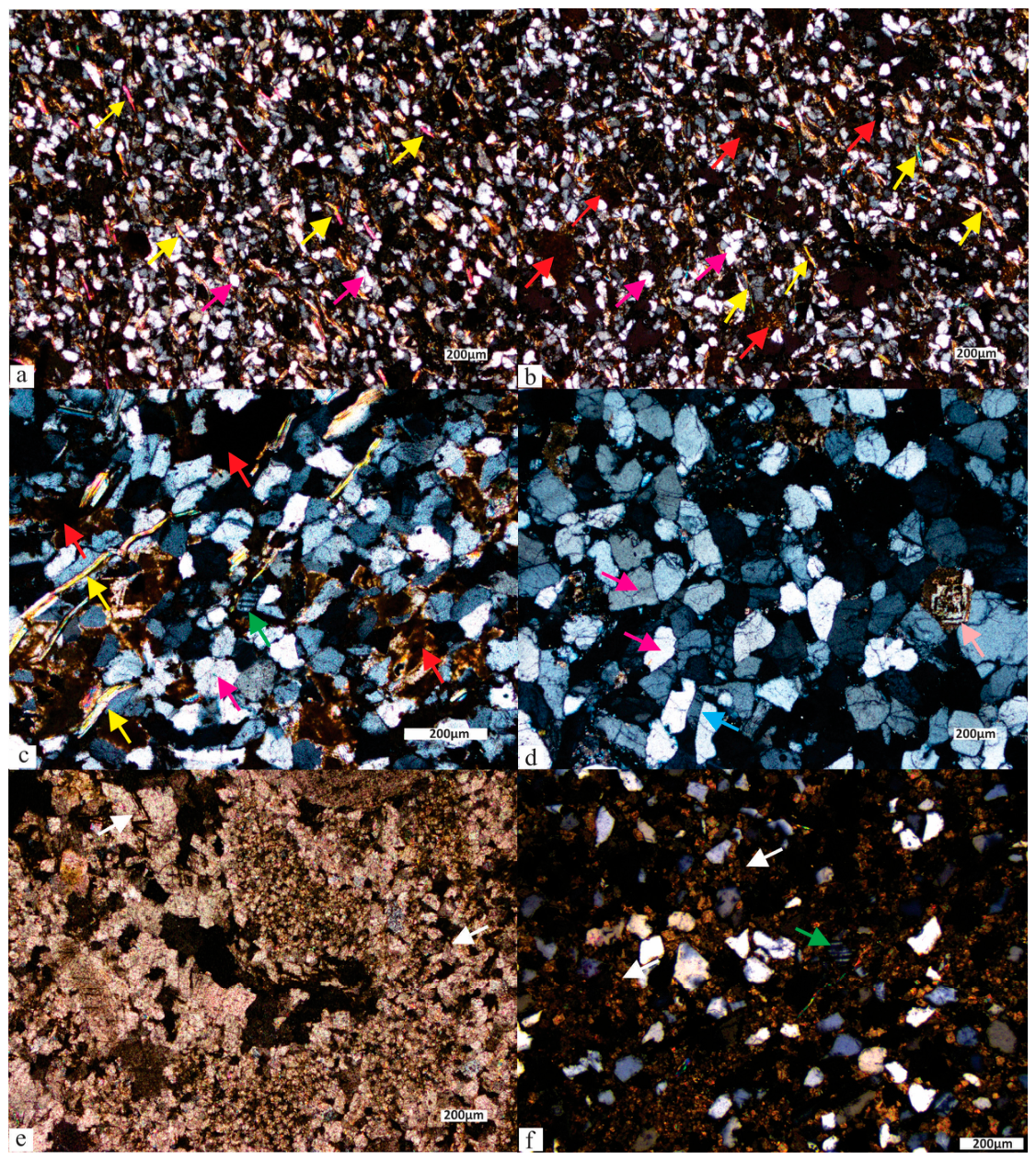
Petrographic studies reveal that in the lower part of the Tredian Formation (LF-1), the sandstones are fine-to-medium-grained and are sub-rounded. The LF-2 sandstones are medium-grained and sub-rounded to well-rounded (Figure 6). Point counting analysis shows that on average, the Tredian Formation consists of 80.1% quartz, 13.9% cement, 3.7% feldspars and 1% lithic fragments (Table 1). Silica and carbonate are the major cement types, along with minor iron oxide. The formation exhibits an overall coarsening upward trend. LF-1 has a grain size ranging from 2.4Ø to 2.8Ø at the Nammal Gorge and 2.5Ø to 2.8Ø at Zaluch Nala (Figure 7 and Figure 8, Table 7). LF-2 has a grain size ranging from 1.5Ø to 2.5Ø at the Nammal Gorge and 1.1Ø to 2.9Ø at Zaluch Nala, and LF-3 contains planer-s (subhedral) and unzoned dolomite and a grain size ranging from 1.2Ø to 1.5Ø at the Nammal Gorge and 1.3Ø to 2Ø at Zaluch Nala (Figure 8, Table 7).

4.3. Grain-Size Statistics

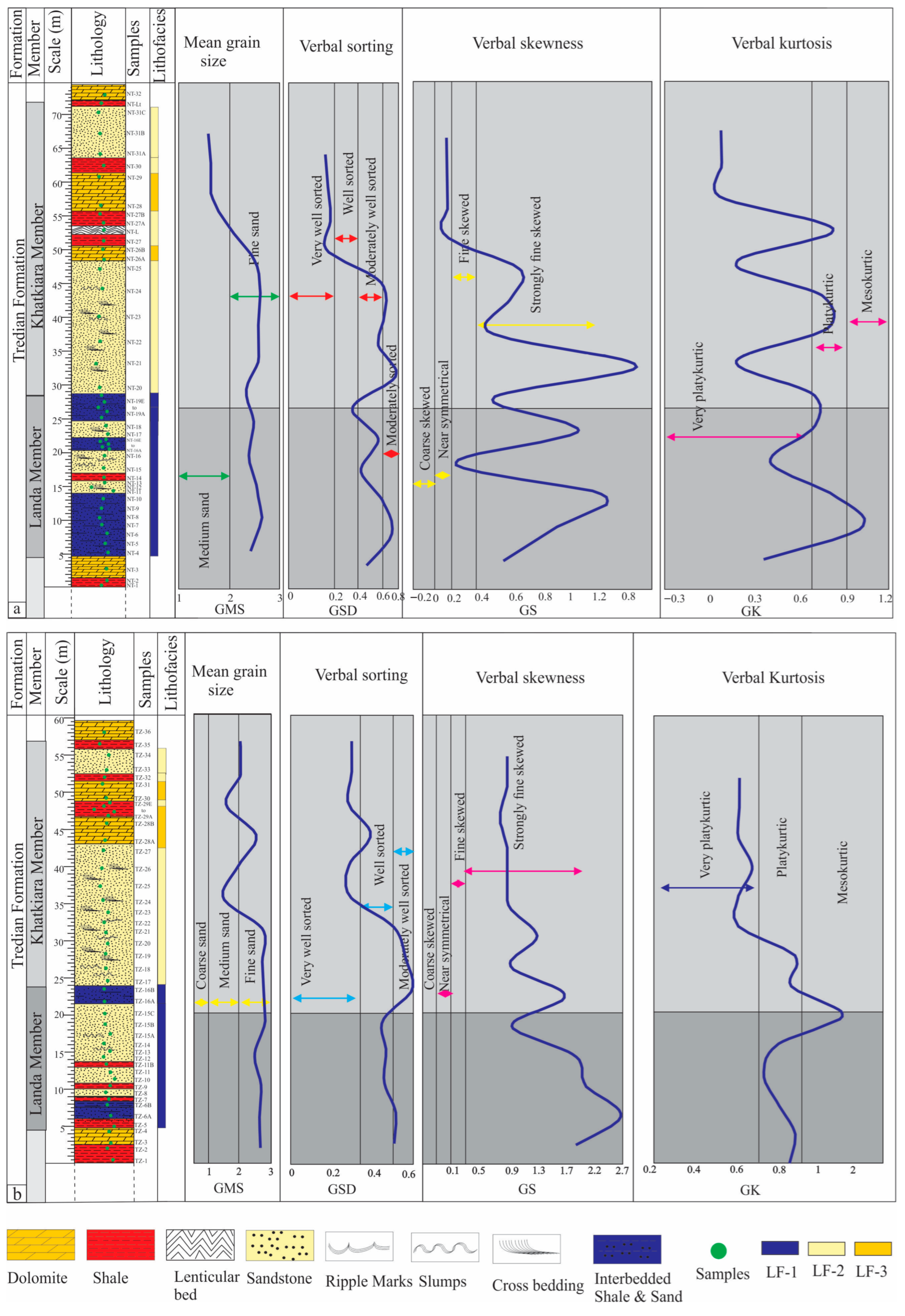
At the Nammal Gorge, most of the sandstone’s grain size in the lower part of the formation ranges from 2.3Ø to 2.7Ø, and in the upper part it ranges from 1.2Ø to 1.9Ø. At Zaluch Nala, sandstones in the lower part range in size from 2.4Ø to 2.83Ø and in the upper part range from 1.1Ø to 2.7Ø (Table 7, Figure 7 and Figure 8). The cumulative volume percentage frequency curve shows a bimodal grain-size distribution in the lower part of the formation, while the upper part displays a unimodal grain-size distribution (Figure 8). The grains display a near-symmetrical distribution. Different grain-size statistical parameters (i.e., mean, standard deviation, skewness, and kurtosis) were calculated from the distribution curves [38]. These parameters were used as input parameters in the DTCM model to present the grain-size characteristics of the Tredian Formation (Table 7, Figure 8).
Figure 8. Vertical variation in grain-size statistical parameters (including graphic mean size, graphic standard deviation, graphic skewness, and graphic kurtosis) across the Tredian Formation. (a) Nammal Gorge and (b) Zaluch Nala.
Minerals 16 00512 g008

4.3.1. Graphic Mean (Mz)

The graphic mean size is related to the overall grain size. The Phi (Ø) graphic mean size represents the average sediment size, which reflects the energy condition index [42]. The calculated graphic mean ranges from 1.21Ø to 2.94Ø at the Nammal Gorge and 1.11Ø to 2.94Ø at Zaluch Nala (Table 7, Figure 8). The average mean grain size of the Tredian Formation in the Salt Range shows the dominance of fine sand, averaging 2.26Ø.

4.3.2. Inclusive Graphic Standard Deviation (σi)

Sorting or uniformity of the grain-size distribution can be measured using the graphic standard deviation. The inclusive graphic standard deviation values in LF-1 ranged from 0.34Ø to 0.52Ø at Zaluch Nala and 0.06Ø to 0.441Ø at the Nammal Gorge. In LF-2, the inclusive graphic standard deviation values ranged from 0.05Ø to 0.90Ø at Zaluch Nala and 0.06Ø to 0.8Ø at the Nammal Gorge. In LF-3, the inclusive graphic standard deviation values ranged from 0.04Ø to 0.34Ø (Table 7, Figure 8).

4.3.3. Inclusive Graphic Skewness (Sk1)

Graphic skewness is the degree of symmetry or asymmetry of the grain-size distribution. The dominance of fine-grained sediments with an asymmetrical curve is said to be positively skewed. If the distribution has a coarse tail (i.e., excess coarse materials), then the sediments are said to be negatively skewed. A symmetrical curve indicates zero phi (Ø), and for near-symmetrical to finely skewed, the inclusive graphic skewness ranges from −0.10Ø to 0.10Ø. For LF-1, the inclusive graphic skewness ranges from 0.15Ø to 1.78Ø, while for LF-2 it ranges from 0.02 to 2.8Ø. LF-3 displays a range from −0.15Ø to 0.01Ø (Table 7, Figure 8).

4.3.4. Graphic Kurtosis (KG)

Kurtosis is a quantitative measure of peakedness in a curve of the grain-size distribution. The graphic kurtosis LF-1 of the Tredian Formation ranges from 0.35Ø to 1.14Ø. In LF-2, the graphic kurtosis values range from 0.01 to 1.59Ø (Figure 8). In LF-3, these values range from 0.002Ø to 0.2Ø at the Nammal Gorge and 0.05Ø to 0.23Ø at Zaluch Nala, which lies in the very platykurtic zone (Table 7, Figure 8). Variations in the graphic kurtosis values take place due to the variation in transportation and depositional medium [43,44].

4.4. Decision Tree Classifier Model (DTCM)

The DTCM classification performance on unseen data and its applicability to the depositional environment interpretation with an accuracy on the testing dataset is shown below (Table 8).
The DTCM shows that the standard deviation (σi) versus mean (Mz) reached an accuracy of 77.78% and an impressive cross-validation accuracy of 96.67%, showing strong generalization despite some misclassification of the minority classes. According to the model, the performance of the “very well sorted” class is superb (F1-score = 0.92), and the performance is clearly lacking for the classes with fewer instances. From the confusion matrix, misclassifications are minor and involve sorting categories that are closely related.
The DTCM for graphic skewness (Sk1) vs. mean (Mz) achieved an accuracy of 57.14%, with cross-validation yielding an accuracy of 68.00%. This illustrates the greater complexity and variability of data pertaining to skewness. With regard to the classification model, predictive performance is good for some classes, like “strongly coarse skewed” (F1-score = 1.00), while other classes, like “near symmetrical”, perform poorly due to overlapping features and a smaller sample size.
The DTCM for graphic kurtosis (KG) vs. mean (MZ) recorded an accuracy of 66.67%, and the F1-score was 0.86, while where the other classes were predicted, the performance was subpar, mainly due to class imbalance and small sample size. The confusion matrix shows misclassification for the skewness classes, which are closely related.
The DTCM model for kurtosis (KG) vs. skewness (SK) achieved 85.71% accuracy and 92.67% accuracy with cross-validation, which demonstrates strong predictive capability. The predictive performance is affected by extreme class imbalance, as most samples belong to the class “very platykurtic.” As a result, macro-average metrics were low despite high accuracy, indicating underperformance in more represented classes.
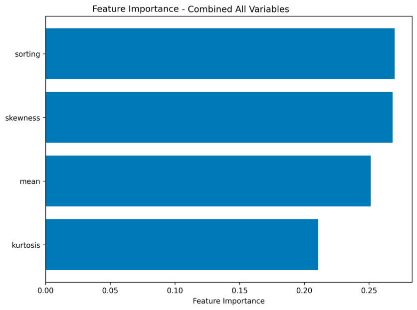
The sample-wise classification results of the DTCM for different grain-size parameter combinations are presented in Table 9, and the relative importance of input variables used in the DTCM is shown in Figure 9.

5. Interpretation and Discussion

5.1. Lithofacies

5.1.1. Sandstone Interbedded with Shale Lithofacies (LF-1)

The ripple marks, cross-bedding, convolute bedding, and parallel lamination reflect the distributary channels’ deposition [25], which are the main components of the delta plain [45]. The scattered pebbles in this lithofacies also support sedimentation in a delta plain setting [46]. The presence of large-scale tabular cross-bedding having the same dipping direction and the foresets inclined in the same direction reflect unidirectional flow with an overall sediment transport from the SE to NW direction (Figure 5). Wave ripple marks indicate the effect of beach actions; however, slumps are uncommon in the shoreline settings, describing it as delta plain lithofacies [47]. Suspension-deposited lamination in fine-grained sediments suggest slow deposition in a quiet water environment in the absence of organic activity (bioturbation), thereby preserving the original lamination [48]. Convolute lamination commonly occurs in turbidities but may also occur in deltaic and fluvial floodplain settings due to channel incision and rolling over of the loose channel margin sediments into the channels/distributary channels [49]. In the present case, the occurrence of slumps/internal contortions can be associated with the instabilities and collapse of the channel margin sediments [25]. Tectonic activities during the passive margin rejuvenation processes may also have contributed to the formation of these slumps in the fluvial–deltaic setting [23]. Channel morphology, cross-bedding, planar lamination, convolute lamination, and slumps support deposition in the distributary channel of delta plain settings, whereas shale was deposited in the low-energy settings of the interdistributary bay/flood plain [25,50]. This interpretation is further supported by the DTCM-based grain-size statistics, which reflect that the sediments related to this lithofacies are moderately well sorted and strongly fine skewed, suggesting the lack of high-energy conditions allowing the deposition of relatively poorly sorted finer sediments [8,44].

5.1.2. Thick-Bedded Sandstone Lithofacies (LF-2)

Large-scale trough and planar tabular cross-bedding, load cast structures, pebbly beds, iron concretion, and medium-grained sandstones in LF-2 (Figure 4 and Figure 5) suggest deposition in high-energy fluvial settings [47,51]. Thick-bedded sandstones can also be deposited through a turbidite ramp system, typically receiving sediments from a deltaic source [46]. Trough cross-bedding is a common sedimentary structure found in channel belt facies of upper and middle delta plain areas, resulting from the migration of large 3D bed forms [52,53]. The observed planar tabular cross-bedding, lenticular channelized structures, and pebbly bases are typically associated with channel bars in fluvial systems and topset areas of deltaic systems [54]. The observed sedimentary structures in LF-2 support deposition in proximal fluvial channel belt settings of a fluvio-deltaic system. The DTCM-based grain-size statistics support this interpretation, where the platykurtic to very leptokurtic sediment of the finer part of LF-2 indicates deposition in the floodplain environment of a fluvial–deltaic system (Figure 8). The fluvial–deltaic system had an overall SE to NW paleoflow direction (Figure 5).

5.1.3. Dolomite Lithofacies (LF-3)

Dolomite may form in lakes or in shallow marine settings [55,56]. This lithofacies indicates fluctuations in sediment supply and current velocity controlled by the environmental conditions. The occurrences of dolomite in the upper part of the Tredian Formation indicate the gradual onset of marine conditions. The lithological variation from pure fluvial sand to sandy dolomite, then to pure dolomite, and finally the transition into the thick dolomite of the Kingriali Formation provides further evidence for the establishment of marine conditions in the area [25]. The presence of lenticular beds indicates that the lithofacies was deposited in lacustrine delta front to shallow marine environments [49]. This interpretation is further supported by the DTCM-based grain-size statistics, which show that F-3 contains near-symmetrical and fine-grained sediments (Figure 8), indicating low-energy deposition in lacustrine/lagoonal subenvironments [48].

5.2. Machine Learning-Based Grain-Size Statistics

The DTCM uses traditional grain-size statistical parameters (i.e., mean size Mz, sorting σi, skewness Sk, and kurtosis KG) as input parameters to categorize depositional environments. This has allowed the integration of machine learning prediction with traditional sedimentology, providing a stronger depositional model. The accuracy and model performance ranged from 57.14% to 85.71%, and cross-validation reached up to 96.67%, reflecting good generalization despite the limitations associated with class imbalance (Table 9). The input parameters for the DTCM contain all key information on the geometric aspects of grains and represent all classified data. Similarly, sediment transport mechanisms and deposition processes are reflected by key bivariate plots that have been used as input parameters to interpret depositional environments [57] and thus to differentiate between fluvial and marine sands [58,59,60,61].
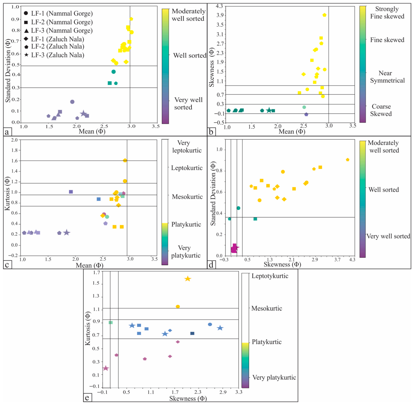
The DTCM-generated bivariate plots of standard deviation (σi) vs. mean (Mz), skewness (Sk1) vs. mean (Mz), kurtosis (KG) vs. mean (Mz), standard deviation (σi) vs. skewness (Sk1), and kurtosis (KG) vs. skewness (Sk1) were used to distinguish depositional settings. In general, the DTCM-generated results for these parameters (Table 9) are consistent with the results of the Linear Discriminant Function (LDF) (discussed later) and suggest a fluvial–deltaic to shallow marine depositional environment, although the DTCM resolves more distinctions among closely related depositional environments.
The DTCM-generated bivariate plot of standard deviation (σi) vs. mean (Mz) shows that the Tredian Formation is dominated by well-sorted (39.3%) and very-well-sorted (35.7%) sandstones, while moderately well-sorted sandstones constitute only 21.4 of the total (Figure 10a). These well-sorted to very-well-sorted sandstones are generally the medium- and coarse-grained sandstones of LF-2 and LF-3, with some contribution from the fine-to-medium-grained sandstones of LF-1 in the lower parts of the formation (Figure 8). The moderately well-sorted sediments that constitute 21.4% of the total samples belong to LF-1 (finer lower part of the formation).
The same medium-to-coarse sandstones of LF-2 and LF-3 are represented by 40% near-symmetrical to coarse-skewed (3.5% are near-symmetrical and 35.71% are coarse-skewed) samples on the graphic skewness (Sk1) vs. mean (Mz) plot (Figure 10b). This DTCM-generated plot helped to improve the lithofacies resolution by separating the 42.85% strongly fine-skewed samples of LF-1 from the rest of the samples.
Well-sorted to very-well-sorted sandstones (Figure 8 and Figure 10a) are generally the products of longer transportation. The relatively coarse-grained sandstones of LF-2 and LF-3 and their unimodal nature indicate a consistent depositional agent characterized by uniform strength of the transporting agent. Such conditions are typical of a fluvial system where channel belt and channel margin facies are deposited [62]. In addition, high-energy waves and currents can produce such well-sorted sediments by continuous reworking of sediments in beach/marginal marine settings [42]. This may support deposition of LF-3 in such transitional settings (lacustrine/marginal marine) with pulses of fluvial influx [25,63]. Thus, the very-well-sorted sandstone and dolomite in the uppermost part of the formation (LF-3) support beach and shallow marine environments before the final onset of marine conditions in which the overlying Kingriali Formation was deposited in the area [64].
The moderately sorted sediments of LF-1 indicated deposition under channel margin, floodplain and lagoonal settings, where the lack of high-energy conditions allows the deposition of relatively poorly sorted finer sediments [8,44]. Positive skewness can be the result of weathering by inducing fine particles [65]. The graphic skewness values vary from strongly fine-skewed to coarse-skewed; such variations show the fluctuation of depositional environments (i.e., seasonal supply of detrital sediments, tidal variation, and wave breaking) [8,66]. The DTCM strengthens this interpretation by linking the LF-1 samples to low-energy settings that are moderately sorted and strongly fine-skewed. On the other hand, the LF-2 and the LF-3 samples are predominantly classified as well-sorted to very-well-sorted, suggesting higher-energy fluvial to marginal marine conditions.
The graphic DTCM display of the kurtosis (KG) vs. mean (MZ) plot shows that 55.5% of the samples are very platykurtic. Such very-platykurtic and very-well-sorted sediments indicate deposition in moderate-to-high-energy depositional environments. In the present case, these represent the samples from the medium-to-coarse-grained sandstones of LF-2 and LF-3, supporting their deposition in high-energy fluvial–deltaic environments with contribution from beach action [8,44,67]. Of the remaining samples, the DTCM indicates that 37% are platykurtic, 3% are mesokurtic, and 3% are very leptokurtic and belong to the fine-grained LF-1, with some contribution from fine-grained sandstones of LF-2 and LF-3. Thus, the platykurtic-to-very-leptokurtic sediments of LF-1 and the finer part of LF-2 indicate deposition in a low-energy channel margin and floodplain environment of a fluvial–deltaic system, while similar sediments in LF-3 indicate low-energy deposition in lacustrine/lagoonal subenvironments [68].
The DTCM-generated bivariate plot of kurtosis (KG) vs. skewness (SK) is a powerful tool to discriminate depositional environments [57]. The DTCM separation on the plot shows that 99% of samples are platykurtic to very platykurtic (i.e., all samples from Zaluch Nala and 13 samples from the Nammal Gorge), and 63% of these are strongly fine-skewed (i.e., seven samples from Zaluch Nala and eight samples from the Nammal Gorge) (Figure 10e). Very platykurtic or extreme leptokurtic reflects that sorting occurred in a fluvial–deltaic setting with contribution from the associated beach and tidal settings [67].
The feature importance (Figure 9) analysis of the DTCM shows that sorting (σi) and skewness (Sk) are the most influential parameters in the classification due to their primary control over hydrodynamic conditions, while mean grain size (Mz) and kurtosis (KG) are of lesser control. In general, the DTCM has enhanced the advanced capabilities of traditional grain-size analysis by introducing an objective, reproducible framework that identifies non-linear relationships within the data, which ultimately improves the confidence associated with the interpretation of depositional environments.

5.3. Linear Discriminant Function (LDF)

The DTCM showed that it is capable of identifying grain-size parameters (sorting, skewness, and kurtosis). In this model, graphic grain-size statistics have been used to construct bivariate and Linear Discriminant Function (LDF) plots to demonstrate grain behaviors.
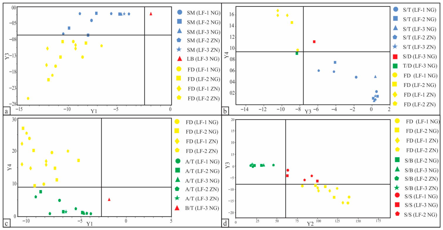
The LDF [39] defines the change in energy and fluidity during deposition. Y1, Y2, Y3, and Y4 are the four LDFs used to discriminate depositional processes and environments. The LDF equations are empirical relationships for differentiating depositional environments. These equations integrate mean grain size, sorting, skewness, and kurtosis into discriminant scores (Y1–Y4) and relate to different sediment transport processes and depositional energy levels.
The functions Y1–Y4 represent dimensionless statistical indices generated through the combination of grain-size parameters. These values are associated with the classification of sediments into a particular depositional environment. Each one captures a defined “process” from a sedimentological perspective:
Y1: Differentiates the aeolian environment from the beach, based on sorting and skewness.
Y2: Differentiates between beach and shallow marine, based on the energy of waves and currents.
Y3: Differentiates between fluvial and deltaic/lacustrine environments, based on the mode of transport and sediment supply.
Y4: Differentiates between turbidity and deltaic depositional environments based on a combination of grain size.
Y1(SA:B) = −3.5688Mz + 3.7016σi2 − 2.0766Sk1 + 3.1135KG
If Y1 is <−2.7411, the environment is aeolian; if it is >−2.7411, the environment is beach.
Y2(SA:B) = 15.653Mz + 65.7091σi2 + 18.1071Sk1 + 18.5043KG
If Y2 is <−63.3650, the environment is beach; if it is >−63.3650, the environment is shallow marine.
Y3(SA:B) = 0.2852Mz − 8.7604σi2 − 4.8932Sk1 + 0.0482KG
If Y3 is >−7.4190, the environment is shallow marine; if it is <−7.4190, the environment is deltaic or lacustrine.
Y4(SA:B) = 0.7215Mz − 0.4030σi2 + 6.7322Sk1 + 5.2927KG
If Y4 is <9.8433, it indicates turbidity current deposition; if it is >9.8433, the environment is deltaic.
In all the equations (i–iv) Mz = mean grain size, σi = standard deviation (sorting), Sk1 = skewness and KG = kurtosis.
Using the LDF, the Tredian Formation yielded Y1 ranging from −1.89 to −11.53, Y2 ranging from 19.55 to 209, Y3 ranging from 0.22 to −27.03 and Y4 ranging from 0.80 to 38.77 (Table 10). Lithofacies LF-1, LF-2 and LF-3 show beach/aeolian processes in Y1 (LDF), with reference to Y2 (LDF) showing a shallow marine environment. In addition, Y3 (LDF) 70% shows fluvial–deltaic and 30% shows shallow marine environments, and in Y4 (LDF) 53% falls in fluvial–deltaic and 47% is in turbidity environments (Table 8).
The binary plot of Y3 versus Y1 shows that 88% of LF-1 was deposited in fluvial–deltaic environments and 12% was deposited in shallow marine environments; LF-2 indicates fluvial–deltaic to shallow marine environments, while samples of LF-3 show that it is deposited in shallow marine environments (Figure 11a). The binary plot of Y3 versus Y2 reflects that 88% of LF-1 supports deposition in fluvial–deltaic to shallow marine environments; LF-2 reflects fluvial—deltaic to shallow marine environments, and LF-3 shows deposition from the surf zone to shallow marine environments (Figure 11d). Similarly, Y4 versus Y3 indicates that LF-1 was deposited in fluvial–deltaic environments and LF-2 and LF-3 in fluvial–deltaic to shallow marine environments (Figure 11b). Y4 versus Y1 shows that LF-1 and LF-2 were deposited in aeolian to fluvial–deltaic environments, and LF-3 was deposited in aeolian to beach/turbidity current environments (Figure 11c).

6. Depositional Settings

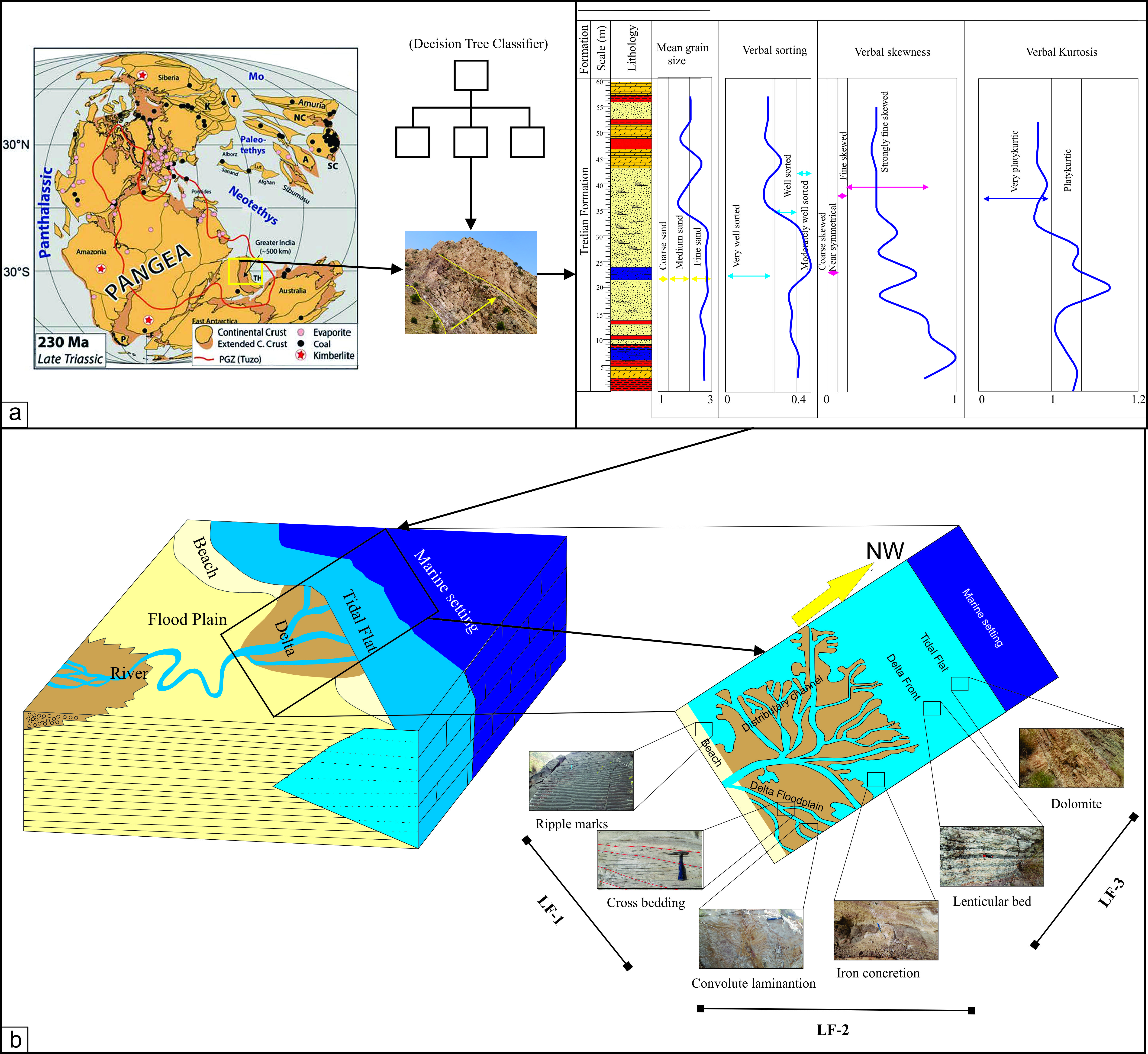
Triassic sedimentation in the Salt Range occurred south of the Neo-Tethyan rift zone [19]. The Middle Triassic Tredian Formation has excellent exposures in the western Salt Range, Surghar Range, and its thickness varies from section to section, which may highlight local tectonic influences or differences in subsidence rates influencing the accommodation space [69]. This period saw episodic tectonic movement and flexural subsidence with regional compressional regimes [23,70]. These created variable accommodation space, which allowed for alternations of fluvial, deltaic, and shallow marine depositional environments [71,72]. The presence of dolomite lithofacies (LF-3) at the top of this formation indicates a relative sea-level rise with a reduction in clastic sedimentation and a stabilization of this sedimentation basin. This is possibly attributable to decreased tectonic disturbances with an increase in marine carbonate sedimentation.
The use of DTCM has established a quantitative method for the reconstruction of depositional environments of the Tredian Formation alongside sedimentological and petrographic studies. The model outputs correlate with the lithofacies interpretation based on field and grain-size data and provide reliable distinctions of delta plain/floodplain deposits (LF-1), fluvial channel deposits (LF-2), and shallow marine to lagoonal deposits (LF-3). The reliability of this model is further attested to by the high accuracy and cross-validation results. The application of machine learning in conjunction with sedimentological studies reduces bias and increases reproducibility and, in this case, provides a marked improvement in the confidence and accuracy of depositional environment reconstruction of the Tredian Formation.
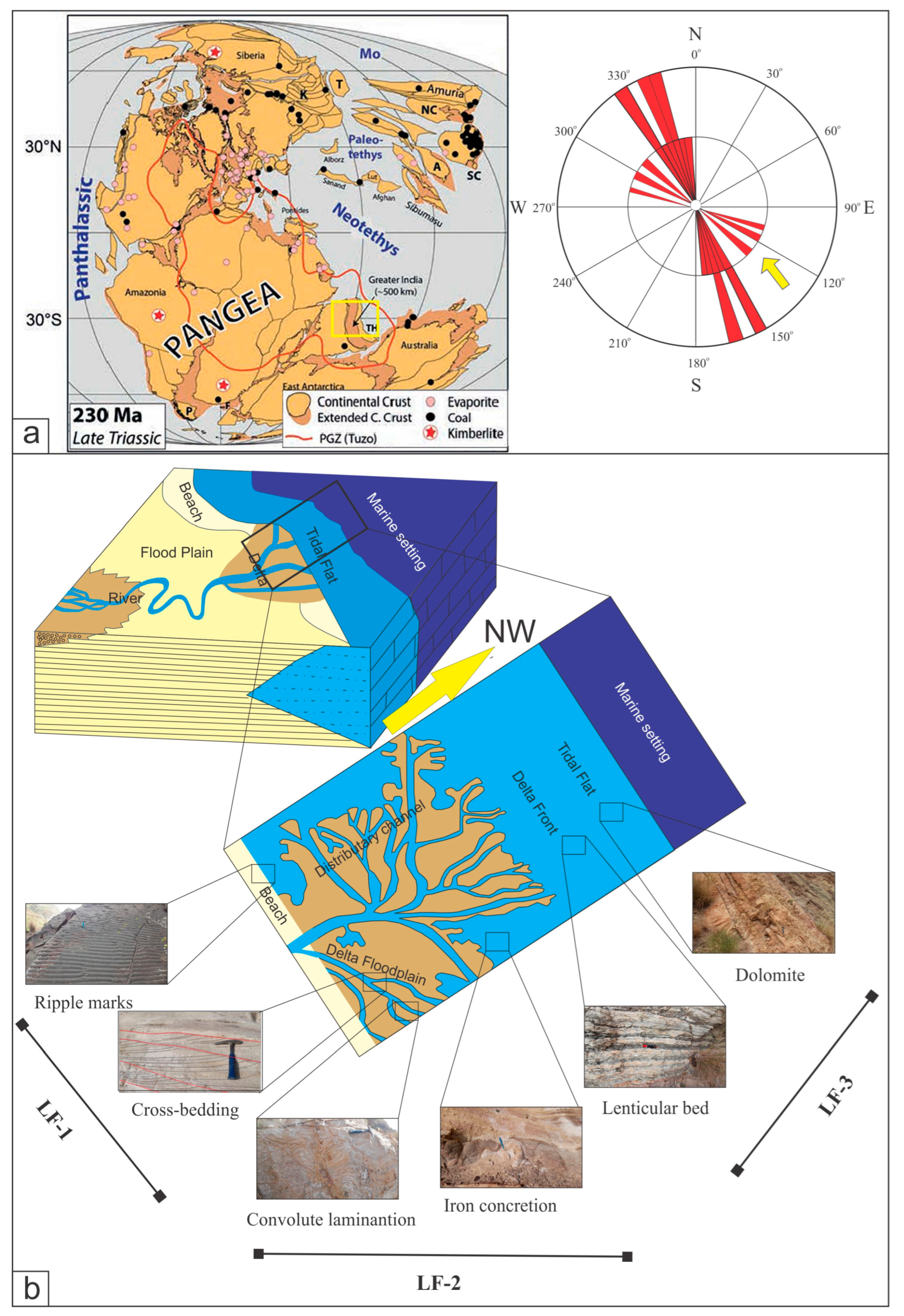
The sandstone interbedded with shale lithofacies (LF-1) reflects deposition in the distributary channel and interdistributary bay of the delta plain settings. The sedimentary structures, including cross-bedding, ripple marks, planar lamination, convolute bedding, and slump of this lithofacies, represent episodic sedimentation. The bimodal flow directions indicate periodic interactions between fluvial–deltaic and deltaic marine processes (Figure 5) [69], while shales are a remnant of low-energy flow deposition in flood plain or interdistributary bay environments (Figure 12).
The deposition of LF-1 was followed by the deposition of thick-bedded sandstone lithofacies (LF-2) from a fluvial channel belt facies association, defined by the presence of large-scale trough and planar cross-bedding, pebbly bases, and channelized geometries. This indicates a vertical transition from deltaic top/delta front deposition to fluvial–deltaic deposition in response to sea-level regression, resulting in coarse-grained facies progradation basinward [24,49]. The paleoflow indicators of LF-1 and LF-2 suggest a SE to NW paleoflow. The lenticular bed between LF-2 and LF-3 and the following thick dolomite beds mark a change in depositional environmental conditions. The dolomite lithofacies (LF-3) support delta front to shallow marine deposition, showing that the transition from fluvial sandstones to sandy dolomites and thick shallow marine dolomite of the Kingriali Formation [25] reflects a reduced siliciclastic input and an increasing marine influence. This succession of the facies in the vertical shows the transgressive timeline, indicating a gradual change from fluvial and delta plain environments to shallow marine settings. The DTCM-based geostatistical results show that the sandstones of the Tredian Formation are very-well-sorted, medium-to-fine-grained, and near-symmetrical to very-platykurtic and indicate deposition in fluvial–deltaic to shallow marine settings (Figure 12).

7. Conclusions

The Tredian Formation has been subdivided into three distinct lithofacies. The basal part of the formation consists of sandstone interbedded with shale lithofacies (LF-1), indicating deposition in a fluvial–deltaic environment, where alternating energy levels of the floodplain/delta top led to the interbedding of shale with sandstones. The thick-bedded sandstone lithofacies (LF-2) represents deposition in a fluvial system, where high-energy conditions and contribution from beach action are found. The dolomite lithofacies (LF-3) suggests deposition in a tidal flat or shallow marine environment. Petrographic-parameter-based machine learning indicates that the sediments are fine-to-medium-grained, moderate-sorting and near-symmetrical to very-platykurtic, which are the characteristics of a fluvial–deltaic to shallow marine setting. The present work indicates that the reconstruction of the depositional setting of the Tredian Formation was achieved through an integrated approach of field observation, grain size and machine learning. The DTCM performance ranged from 57.14% to 85.71% and cross-validation reached up to 96.67%, reflecting good generalization of the depositional environments interpretation. Overall, the DTCM and LDF reveal low energy depositions for the lower part of the Tredian Formation (LF-1) and higher-energy fluvial to marginal marine environments for the upper part of the formation (LF-2 and LF-3). The feature importance analysis of the DTCM shows that sorting (σi) and skewness (Sk) are the most influential parameters in the classification due to their primary control over hydrodynamic conditions, while mean grain size (Mz) and kurtosis (KG) are of lesser control.

Supplementary Materials

The following supporting information can be downloaded at: https://www.mdpi.com/article/10.3390/min16050512/s1, Source code for all the key parameters and plots, including: mean (Mz) vs. kurtosis (KG); skewness (Sk) vs. kurtosis (KG); skewness (Sk) vs. mean (Mz); sorting (σi) vs. mean (Mz); sorting vs. skewness be downloaded in the website.

Author Contributions

Conceptualization, M.I. and S.I.; methodology, S.I., M.I. and M.W.; software, M.I., M.A. and M.B.; validation, S.I., M.W., M.I. and M.B.; formal analysis, M.I., A.B.Q. and B.W.; investigation, M.I., A.B.Q., S.I., M.B., B.W. and M.A.; resources, S.I., M.W. and M.B.; data curation, M.I. and M.A.; writing—original draft preparation, M.I. and S.I.; writing—review and editing, M.I., S.I., M.W. and M.B.; visualization, M.I., S.I., M.W. and M.B.; supervision, S.I. and M.W.; project administration, S.I.; funding acquisition, S.I., M.W. and M.B. All authors have read and agreed to the published version of the manuscript.

Funding

The Department of Earth Sciences, Quaid-i-Azam University, Islamabad, provided logic support for the fieldwork. IGCP-732 provided financial support for sample collection and thin-section preparation. The APC was funded by the University of Vienna.

Data Availability Statement

Data have been included in the tables within the manuscript.

Acknowledgments

This research is a part of the PhD study of the corresponding author. The authors are thankful to Saima Jabeen, Jansher Khan, and Muhammad Bilal for their help with thin-section preparation.

Conflicts of Interest

The authors declare no conflicts of interest.

Abbreviations

The following abbreviations are used in this manuscript:
MLMachine Learning
SOMsSelf-Organizing Maps
UVQ–ANNUnsupervised Vector Quantizer Artificial Neural Network
SISSequential Indicator Simulation
DTCMDecision Tree Classifier Model
HFTBHimalayan Fold and Thrust Belt
SRTSalt Range Thrust
LF-1Sandstone Interbedded with shale lithofacies
LF-2Thick-Bedded Sandstone Lithofacies
LF-3Dolomite lithofacies
GSPGeological Survey of Pakistan
BKUCBacha Khan University, Charsadda
NCEGNational Centre of Excellence in Geology
QtTotal Quartz
QmueMonocrystalline Quartz with unit extinction
QmuuMonocrystalline Quartz with undulose extinction
Qpq(2–3)Polycrystalline Quartz with 2–3 crystals
Qpq>3Polycrystalline Quartz with >3 crystals
FFeldspar
LLithic Fragments
LDFLinear Discriminant Function
SESoutheast
NWNorthwest
ICIron Concretion
σiStandard Deviation
MzMean
SkSkewness
KKurtosis

References

  1. Anifowose, F.; Abdulraheem, A.; Al-Shuhail, A. A parametric study of machine learning techniques in petroleum reservoir permeability prediction by integrating seismic attributes and wireline data. J. Pet. Sci. Eng. 2019, 176, 762–774. [Google Scholar] [CrossRef]
  2. Duch, W.; Adamczak, R.; Jankowski, N. Initialization and optimization of multilayered perceptrons. In Proceedings of the Third Conference on Neural Networks and Their Applications, Kule, Poland, 14–18 October 1997; pp. 99–104. [Google Scholar]
  3. Hosmer, D.W.; Lemeshow, S.; Sturdivant, R.X. Applied Logistic Regression; Wiley: New York, NY, USA, 2000. [Google Scholar]
  4. Koeshidayatullah, A.; Al-Azani, S.; Baraboshkin, E.E.; Alfarraj, M. FaciesVit: Vision transformer for an improved core lithofacies prediction. Front. Earth Sci. 2022, 10, 992442. [Google Scholar] [CrossRef]
  5. Yang, M.; Hu, Y.; Liu, B.; Wang, L.; Zhou, Z.; Jia, M. Application of Artificial Neural Networks for Identification of Lithofacies by Processing of Core Drilling Data. Appl. Sci. 2023, 13, 11934. [Google Scholar] [CrossRef]
  6. Shi, X.; Liu, J.; Zhu, Y.; Xu, L.; Yang, Y.; Luo, C.; Li, Y.; Zhong, K.; Yang, X.; Wu, Q.; et al. Effects of the Sedimentary Environment on Organic-Rich Shale in the Intracratonic Sag of the Sichuan Basin, China. Appl. Sci. 2024, 14, 8594. [Google Scholar] [CrossRef]
  7. Khalil, R. Grain-size analysis of middle Cretaceous sandstone reservoirs, the Wasia formation, Riyadh province, Saudi Arabia. Sustainability 2023, 15, 7983. [Google Scholar] [CrossRef]
  8. Baiyegunhi, C.; Liu, K.; Gwavava, O. Grain size statistics and depositional pattern of the Ecca Group sandstones, Karoo Supergroup in the Eastern Cape Province, South Africa. Open Geosci. 2017, 9, 554–576. [Google Scholar] [CrossRef]
  9. Baiyegunhi, T.L.; Liu, K.; Gwavava, O.; Baiyegunhi, C. Textural characteristics, mode of transportation and depositional environment of the Cretaceous sandstone in the Bredasdorp Basin, off the south coast of South Africa: Evidence from grain size analysis. Open Geosci. 2020, 12, 1512–1532. [Google Scholar] [CrossRef]
  10. Demyanov, V.; Reesink, A.J.H.; Arnold, D.P. Can machine learning reveal sedimentological patterns in river deposits? Geol. Soc. Lond. Spec. Publ. 2019, 488, 221–235. [Google Scholar] [CrossRef]
  11. Hussain, M.; Liu, S.; Ashraf, U.; Ali, M.; Hussain, W.; Ali, N.; Anees, A. Application of machine learning for lithofacies prediction and cluster analysis approach to identify rock type. Energies 2022, 15, 4501. [Google Scholar] [CrossRef]
  12. Tang, D.G.; Milliken, K.L.; Spikes, K.T. Machine learning for point counting and segmentation of arenite in thin section. Mar. Pet. Geol. 2020, 120, 104518. [Google Scholar] [CrossRef]
  13. Ashraf, U.; Zhang, H.; Anees, A.; Mangi, H.N.; Ali, M.; Zhang, X.; Imraz, M.; Abbasi, S.S.; Abbas, A.; Ullah, Z.; et al. A core logging, machine learning and geostatistical modeling interactive approach for subsurface imaging of lenticular geobodies in a clastic depositional system, SE Pakistan. Nat. Resour. Res. 2021, 30, 2807–2830. [Google Scholar] [CrossRef]
  14. Ghazi, S.; Ali, S.H.; Sahraeyan, M.; Hanif, T. An overview of tectonosedimentary framework of the Salt Range, northwestern Himalayan fold and thrust belt, Pakistan. Arab. J. Geosci. 2015, 8, 1635–1651. [Google Scholar] [CrossRef]
  15. Iqbal, S.; Akhter, G.; Bibi, S. Structural model of the Balkassar area, Potwar Plateau, Pakistan. Int. J. Earth Sci. 2015, 104, 2253–2272. [Google Scholar] [CrossRef]
  16. Kazmi, A.H.; Jan, M.Q. Geology and Tectonics of Pakistan; Graphic Publishers: Karachi, Pakistan, 1997; 554p. [Google Scholar]
  17. Kazmi, A.; Abbasi, I. Stratigraphy and Historical Geology of Pakistan: National Centre of Excellence in Geology; University of Peshawar: Peshawar, Pakistan, 2008; 524p. [Google Scholar]
  18. Qasim, M.; Ahmad, J.; Ding, L.; Tanoli, J.I.; Sattar, M.; Rehman, Q.U.; Awais, M.; Umar, M.; Baral, U.; Khan, H. Integrated provenance and tectonic implications of the Cretaceous–Palaeocene clastic sequence, Changla Gali, Lesser Himalaya, Pakistan. Geol. J. 2021, 56, 4747–4759. [Google Scholar] [CrossRef]
  19. Hermann, E.; Hochuli, P.A.; Bucher, H.; Vigran, J.O.; Weissert, H.; Bernasconi, S.M. A close-up view of the Permian–Triassic boundary based on expanded organic carbon isotope records from Norway (Trøndelag and Finnmark Platform). Glob. Planet. Change 2010, 74, 156–167. [Google Scholar] [CrossRef]
  20. Galfetti, T.; Bucher, H.; Brayard, A.; Hochuli, P.A.; Weissert, H.; Guodun, K.; Atudorei, V.; Guex, J. Late Early Triassic climate change: Insights from carbonate carbon isotopes, sedimentary evolution and ammonoid paleobiogeography. Palaeogeogr. Palaeoclimatol. Palaeoecol. 2007, 243, 394–411. [Google Scholar] [CrossRef]
  21. Kutzbach, J.; Gallimore, R.G. Pangaean climates: Megamonsoons of the megacontinent. J. Geophys. Res. Atmos. 1989, 94, 3341–3357. [Google Scholar] [CrossRef]
  22. Baud, A.; Atudorei, V.; Sharp, Z. Late Permian and Early Triassic evolution of the Northern Indian margin: Carbon isotope and sequence stratigraphy. Geodin. Acta 1996, 9, 57–77. [Google Scholar] [CrossRef]
  23. Iqbal, S.; Wagreich, M.; Bibi, M.; Jan, I.U.; Gier, S. Multi-proxy provenance analyses of the Kingriali and Datta formations (Triassic–Jurassic transition): Evidence for westward extension of the Neo-Tethys passive margin from the Salt Range (Pakistan). Minerals 2021, 11, 573. [Google Scholar] [CrossRef]
  24. Qureshi, K.A.; Arif, M.; Basit, A.; Ahmad, S.; Janjuhah, H.T.; Kontakiotis, G. Sedimentological controls on the reservoir characteristics of the mid-Triassic Tredian Formation in the salt and trans-Indus Surghar Ranges, Pakistan: Integration of outcrop, petrographic, and SEM analyses. J. Mar. Sci. Eng. 2023, 11, 1019. [Google Scholar] [CrossRef]
  25. Iqbal, S.; Jan, I.U.; Hanif, M. The Mianwali and Tredian formations: An example of the Triassic progradational deltaic system in the low-latitude western Salt Range, Pakistan. Arab. J. Sci. Eng. 2014, 39, 5489–5507. [Google Scholar] [CrossRef]
  26. Shah, S. Stratigraphy of Pakistan. In Memoirs of the Geological Survey of Pakistan; Government of Pakistan, Ministry of Petroleum and Natural Resources, Geological Survey of Pakistan: Islamabad, Pakistan, 2009; Volume 22. [Google Scholar]
  27. Mertmann, D. Evolution of the marine Permian carbonate platform in the Salt Range (Pakistan). Palaeogeogr. Palaeoclimatol. Palaeoecol. 2003, 191, 373–384. [Google Scholar] [CrossRef]
  28. Iqbal, S.; Wagreich, M.; Kuerschner, W.M.; Gier, S.; Bibi, M. Hot-house climate during the Triassic/Jurassic transition: The evidence of climate change from the southern hemisphere (Salt Range, Pakistan). Glob. Planet. Change 2019, 172, 15–32. [Google Scholar] [CrossRef]
  29. Ahmad, I.; Shah, M.M.; Janjuhah, H.T.; Trave, A.; Antonarakou, A.; Kontakiotis, G. Multiphase diagenetic processes and their impact on reservoir character of the Late Triassic (Rhaetian) Kingriali Formation, Upper Indus Basin, Pakistan. Minerals 2022, 12, 1049. [Google Scholar] [CrossRef]
  30. DeCelles, P.G.; Langford, R.P.; Schwartz, R.K. Two new methods of paleocurrent determination from trough cross-stratification. J. Sediment. Res. 1983, 53, 629–642. [Google Scholar] [CrossRef]
  31. Kadri, I.B. Petroleum Geology of Pakistan; Pakistan Petroleum Limited: Karachi, Pakistan, 1995; 275p. [Google Scholar]
  32. Adams, J. Sieve size statistics from grain measurement. J. Geol. 1977, 85, 209–227. [Google Scholar] [CrossRef]
  33. Johnson, M. Thin section grain size analysis revisited. Sedimentology 1994, 41, 985–999. [Google Scholar] [CrossRef]
  34. Liu, K.; Greyling, E. Grain-size distribution and cementation of the Cretaceous Mzamba Formation of Eastern Cape, South Africa: A case study of a storm-influenced offshore sequence. Sediment. Geol. 1996, 107, 83–97. [Google Scholar] [CrossRef]
  35. Udden, J.A. Mechanical composition of clastic sediments. Bull. Geol. Soc. Am. 1914, 25, 655–744. [Google Scholar] [CrossRef]
  36. Wentworth, C.K. Method of computing mechanical composition types in sediments. Bull. Geol. Soc. Am. 1929, 40, 771–790. [Google Scholar] [CrossRef]
  37. Abuodha, J. Grain size distribution and composition of modern dune and beach sediments, Malindi Bay coast, Kenya. J. Afr. Earth Sci. 2003, 36, 41–54. [Google Scholar] [CrossRef]
  38. Folk, R.L.; Ward, W.C. Brazos River bar [Texas]; a study in the significance of grain size parameters. J. Sediment. Res. 1957, 27, 3–26. [Google Scholar] [CrossRef]
  39. Sahu, B.K. Depositional mechanisms from the size analysis of clastic sediments. J. Sediment. Res. 1964, 34, 73–83. [Google Scholar] [CrossRef]
  40. Folk, R.L. Petrology of Sedimentary Rocks; Hemphill Publishing Company: Austin, TX, USA, 1980. [Google Scholar]
  41. Utkin, L.V.; Coolen, F.P. Interval-valued regression and classification models in the framework of machine learning. In Proceedings of the 7th International Symposium on Imprecise Probability: Theories and Applications, Innsbruck, Austria, 25–28 July 2011. [Google Scholar]
  42. Passega, R. Grain size representation by CM patterns as a geologic tool. J. Sediment. Res. 1964, 34, 830–847. [Google Scholar] [CrossRef]
  43. Seralathan, P.; Padmalal, D. Textural studies of the surficial sediments of Muvattupuzha river and central Vembanad Estuary, Kerala. J. Geol. Soc. India 1994, 43, 179–190. [Google Scholar] [CrossRef]
  44. Kotoky, J.B.P.; Sarma, J. A Case Study on the Jhanji river, Assam. J. Indian Assoc. Sedimentol. 1997, 16, 195–206. [Google Scholar]
  45. Kästner, K.; Hoitink, A.J.F.; Vermeulen, B.; Geertsema, T.J.; Ningsih, N.S. Distributary channels in the fluvial to tidal transition zone. J. Geophys. Res. Earth Surf. 2017, 122, 696–710. [Google Scholar] [CrossRef]
  46. Reading, H.G. Sedimentary Environments: Processes, Facies and Stratigraphy; John Wiley & Sons: Hoboken, NJ, USA, 2009; 669p. [Google Scholar]
  47. Mehmood, M.; Naseem, A.A.; Saleem, M.; Rehman, J.U.; Kontakiotis, G.; Janjuhah, H.T.; Khan, E.U.; Antonarakou, A.; Khan, I.; Rehman, A.U.; et al. Sedimentary facies, architectural elements, and depositional environments of the Maastrichtian Pab Formation in the Rakhi Gorge, Eastern Sulaiman Ranges, Pakistan. J. Mar. Sci. Eng. 2023, 11, 726. [Google Scholar] [CrossRef]
  48. Hesse, R.; Chough, S.K. The Northwest Atlantic Mid-Ocean Channel of the Labrador Sea: II. Deposition of parallel laminated levee-muds from the viscous sublayer of low density turbidity currents. Sedimentology 1980, 27, 697–711. [Google Scholar] [CrossRef]
  49. Boggs, S., Jr. Petrology of Sedimentary Rocks; Cambridge University Press: Cambridge, UK, 2009. [Google Scholar] [CrossRef]
  50. Nichols, G. Sedimentology and Stratigraphy Blackwell Publishing; John Wiley & Sons, Ltd. Publication: London, UK, 1999. [Google Scholar]
  51. Eriksson, P.G.; Condie, K.C.; Tirsgaard, H.; Mueller, W.U.; Altermann, W.; Miall, A.D.; Aspler, L.B.; Catuneanu, O.; Chiarenzelli, J.R. Precambrian clastic sedimentation systems. Sediment. Geol. 1998, 120, 5–53. [Google Scholar] [CrossRef]
  52. Allison, M.A.; Khan, S.R.; Goodbred, S.L., Jr.; Kuehl, S.A. Stratigraphic evolution of the late Holocene Ganges–Brahmaputra lower delta plain. Sediment. Geol. 2003, 155, 317–342. [Google Scholar] [CrossRef]
  53. Scasso, R.A.; Aberhan, M.; Ruiz, L.; Weidemeyer, S.; Medina, F.A.; Kiessling, W. Integrated bio-and lithofacies analysis of coarse-grained, tide-dominated deltaic environments across the Cretaceous/Paleogene boundary in Patagonia, Argentina. Cretac. Res. 2012, 36, 37–57. [Google Scholar] [CrossRef]
  54. Friedman, G.M.; Sanders, J.E. Principles of Sedimentology; Wiley: New York, NY, USA, 1978; 218p. [Google Scholar]
  55. Meister, P.; Mckenzie, J.A.; Bernasconi, S.M.; Brack, P. Dolomite formation in the shallow seas of the Alpine Triassic. Sedimentology 2013, 60, 270–291. [Google Scholar] [CrossRef]
  56. Blendinger, W.; Lohmeier, S.; Bertini, A.; Meißner, E.; Sattler, C.D. A new model for the formation of Dolomite in the Triassic dolomites, Northern Italy. J. Pet. Geol. 2015, 38, 5–36. [Google Scholar] [CrossRef]
  57. Friedman, G.M. Dynamic processes and statistical parameters compared for size frequency distribution of beach and river sands. J. Sediment. Res. 1967, 37, 327–354. [Google Scholar] [CrossRef]
  58. Al-Ghadban, A. Holocene sediments in a shallow bay, southern coast of Kuwait, Arabian Gulf. Mar. Geol. 1990, 92, 237–254. [Google Scholar] [CrossRef]
  59. Sutherland, R.A.; Lee, C.T. Discrimination between coastal subenvironments using textural characteristics. Sedimentology 1994, 41, 1133–1145. [Google Scholar] [CrossRef]
  60. Martins, L. Recent sediments and grain-size analysis. Gravel 2003, 1, 90–105. [Google Scholar]
  61. Srivastava, A.K.; Ingle, P.S.; Lunge, H.S.; Khare, N. Grain-size characteristics of deposits derived from different glacigenic environments of the Schirmacher Oasis, East Antarctica. Geologos 2012, 18, 251–266. [Google Scholar] [CrossRef][Green Version]
  62. Rajganapathi, V.; Jitheshkumar, N.; Sundararajan, M.; Bhat, K.H.; Velusamy, S. Grain size analysis and characterization of sedimentary environment along Thiruchendur coast, Tamilnadu, India. Arab. J. Geosci. 2013, 6, 4717–4728. [Google Scholar] [CrossRef]
  63. Edwards, A.C. Grain size and sorting in modern beach sands. J. Coast. Res. 2001, 17, 38–52. [Google Scholar]
  64. Preoteasa, L.; Vespremeanu-Stroe, A. Grain-Size Analysis of the Beach-Dune Sediments and the Geomorphological Significance. Rev. Geomorfol. 2010, 12, 73–79. [Google Scholar]
  65. Yang, H.; Shi, C. Sediment grain-size characteristics and its sources of ten wind-water coupled erosion tributaries (the Ten Kongduis) in the Upper Yellow River. Water 2019, 11, 115. [Google Scholar] [CrossRef]
  66. Selvaraj, K.; Mohan, V.R. Textural variation and depositional environments of innershelf sediments, off Kalpakkam, southeast coast of India. J. Geol. Soc. India 2003, 61, 449–462. [Google Scholar] [CrossRef]
  67. Friedman, G.M. Distinction between dune, beach, and river sands from their textural characteristics. J. Sediment. Res. 1961, 31, 514–529. [Google Scholar] [CrossRef]
  68. Elshahat, O. Sedimentological and Heavy Minerals Studies on Stream Sediments, El-Sheikh Abdelal Tomb-El-Fawakhir, Central Eastern Desert, Egypt. Egypt. J. Geol. 2018, 62, 269–282. [Google Scholar]
  69. Collinson, J.; Mountney, N. Sedimentary Structures; Liverpool University Press: Liverpool, UK, 2019; 352p. [Google Scholar]
  70. Torsvik, T.H.; Cocks, L.R.M. Earth History and Palaeogeography; Cambridge University Press: Cambridge, UK, 2017; p. 317. [Google Scholar] [CrossRef]
  71. Wang, J.; La Croix, A.D.; Wang, H.; Fu, Y.; Fan, Z. Compression-induced evolution of the Triassic stratigraphy and sedimentary facies in the backbulge depression of the Tarim Basin, NW China. J. Asian Earth Sci. 2026, 302, 107023. [Google Scholar] [CrossRef]
  72. Saboor, A.; Haq, M.U.; Nawaz, A.; Swati, M.A.F.; Gohar, J.; Khan, S.; Ghaffari, A. Insight to the geological character of the Early Triassic strata in the Western Salt Range, Pakistan: A comparative study. Geol. J. 2021, 56, 4667–4684. [Google Scholar] [CrossRef]
Figure 6. Photomicrographs of the sandstones of the Tredian Formation. (a) LF-1 (Zaluch Nala), yellow arrow pointing to mica, magenta arrow pointing to quartz; (b) LF-1 (Nammal Gorge), yellow arrow pointing to mica, red arrow pointing to matrix, magenta arrow pointing to quartz; (c) LF-2 (Zaluch Nala) yellow arrow pointing to mica, green arrow pointing to feldspar (plagioclase), magenta arrow pointing to quartz, red arrow pointing to matrix; (d) LF-2 (Nammal Gorge), blue arrow pointing to long-linear contacts between quartz grains, magenta arrow pointing to quartz, pink arrow pointing to lithic clast; (e) LF-3 (Zaluch Nala), white arrow pointing to dolomite; (f) LF-3 (Nammal Gorge), green arrow pointing to feldspar in the sandy dolomite, white arrow pointing to dolomite.
Minerals 16 00512 g006
Figure 7. Graphical representation of statistical parameters for a representative sample (NT-25) of the Tredian Formation: (a) grain-size frequency histogram; (b) cumulative frequency curve (blue line) showing the method for calculating percentile values (red lines).
Minerals 16 00512 g007
Figure 9. The feature importance of input parameters in the DTCM showing the relative contribution of each variable.
Minerals 16 00512 g009
Figure 10. Machine learning (ML) Decision Tree Classifier Model (DTCM) color-coded based on (a) bivariate plot of graphic standard deviation vs. graphic mean, (b) bivariate plot of graphic skewness vs. graphic mean, (c) bivariate plot of graphic kurtosis vs. graphic mean, (d) bivariate plot of standard deviation or sorting vs. graphic skewness and (e) bivariate plot of graphic kurtosis vs. graphic skewness.
Minerals 16 00512 g010
Figure 11. Machine learning Decision Tree Classifier Model (DTCM) color-coded based on the following: (a) discrimination of environments based on Linear Discriminant Function (LDF) plot pf Y3 versus Y1. (b) Discrimination of environments based on LDF plot of Y4 versus Y3. (c) Discrimination of environments based on LDF plot of Y4 versus Y1. (d) Discrimination of environments based on LDF plot of Y3 versus Y2. SM = shallow marine, LB = littoral–beach, FD = fluvial–deltaic, S/T = shallow marine/turbidity currents, S/D = shallow marine–deltaic, T/D = turbidity currents/deltaic, A/T = aeolian/turbidity currents, B/T = beach/turbidity currents, SB = shallow marine/beach, S/S = surf zone/shallow marine.
Minerals 16 00512 g011
Figure 12. (a) Paleogeographic position of the Salt Range and paleoflow direction during the deposition of the Tredian Formation during the Middle Triassic [70]. The yellow box marks the Salt Range. (b) Schematic depositional model for the Tredian Formation. The yellow arrow indicates the paleoflow direction.
Minerals 16 00512 g012
Table 1. Framework mineralogical composition of the Tredian Formation. Q = total quartz, Qmue = monocrystalline quartz with unit extinction, Qmuu = monocrystalline quartz with undulose extinction, Qpq(2–3) = polycrystalline quartz with 2–3 crystals, Qpq>3 = polycrystalline quartz with >3 crystals, F = feldspar and L = lithic fragments. Please note that 500 grains were counted for each sample.
Sample IDQ = Qmue + Qmuu + Qpq(2–3) + Qpq>3FLCementsTotal
QQmueQmuuQpq(2–3)Qpq>3
NT-5405375205520570500
NT-8435390251010151040500
NT-113953602051020085500
NT-13424389227517357500
NT-154453904010510540500
NTS-15c438396271149647500
NT-16396361216423679500
NT-16c411376186621667500
NT-174153554515520555500
NT-18423389276417354500
NT-20387357173728880500
NT-213903651555301565500
NT-23428397267417346500
NT-253653550552010105500
NT-27398362164725482500
NT-30394366145723580500
TZ-340036520510101080500
TZ-437535010105301778500
TZ-64303952555251530500
TZ-84504003551015530500
TZ-11425395205510560500
TZ-13413378183713477500
TZ-1445041515101010530500
TZ-15402372166522376500
TZ-20382352184424494500
TZ-2741038015510451530500
TZ-28422387196727549500
TZ-3039537551055595500
TZ-333653500105182115500
TZ-34392362166522386500
Average %81.8%75.18%3.87%1.5%1.3%3.78%1.6%12.5%100%
Table 2. Equations for calculating grain-size parameters by graphical methods [38].
Graphic Mean (Mz)Mz = Ø 16 + Ø 50 + Ø 84 3
Inclusive Graph Standard Deviation (σi)σi = Ø 84 Ø 16 4 + Ø 95 Ø 5 6.6
Inclusive Graph Skewness (Ski)Ski = ( Ø 84 + Ø 16 2 Ø 50 ) 2 ( Ø 84 Ø 16 ) + ( Ø 95 + Ø 5 2 Ø 50 ) 2 ( Ø 95 Ø 5 )
Graphic Kurtosis (KG)KG = ( Ø 95 Ø 5 ) 2.44 ( Ø 74 Ø 25 )
In the equations, Ø5, Ø16, Ø25, Ø50, Ø75, Ø84, and Ø95 represent the 5th, 16th, 25th, 50th, 75th, 84th, and 95th percentiles, respectively, on the cumulative curve.
Table 3. Verbal terms for sorting and the corresponding values of the inclusive graphic standard deviation [40].
Phi Standard DeviationVerbal Sorting
<0.35 ØVery well sorted
0.35 to 0.50 ØWell sorted
0.50 to 0.70 ØModerately well sorted
0.70 to 1.00 ØModerately sorted
1.00 to 2.00 ØPoorly sorted
2.00 to 4.00 ØVery poorly sorted
˃4.00 ØExtremely poorly sorted
Table 4. Verbal terms for skewness and the corresponding value of the calculated skewness [40].
Calculated SkewnessVerbal Skewness
˃+0.30 Strongly fine skewed
+0.30 to 0.10Fine skewed
+0.10 to −0.10Near symmetrical
−0.10 to −0.30 Coarse skewed
<−0.30Strongly coarse skewed
Table 5. Verbal terms for kurtosis and the corresponding value of the calculated kurtosis [40].
Calculated KurtosisVerbal Kurtosis
<0.67Very platykurtic
0.67 to 0.90 Platykurtic
0.90 to 1.11Mesokurtic
1.11 to 1.50 Leptokurtic
1.50 to 3.00 Very leptokurtic
˃3.00Extremely leptokurtic
Table 6. Details of lithofacies of the Tredian Formation in the studied sections.
LithofaciesDescriptionInterpretation
Sandstone interbedded with shale lithofacies (LF-1)Medium-to-thick-bedded sandstone interbedded with black shale; cross-bedding, parallel lamination, ripple marks, both symmetrical and asymmetrical, slumps, and flame structures Deposition in the distributary channels, delta top/flood plain,
Thick-bedded sandstone Lithofacies (LF-2)Fine-to-medium-thick-bedded sandstone having cross-bedding (planar and trough), load marks, and ripple marksHigh fluvial discharge in a channel belt environment during delta progradation
Dolomite lithofacies
(LF-3)
Brown, yellowish, and medium-bedded dolomite, with a sandy lower part, pure dolomite in the upper partDeposition in fluctuating shallow depositional conditions
Table 7. Graphic measures and grain-size parameters for the selected samples from the Tredian Formation.
Sample IDMedian (Md)Mean (M)Sorting (σØ)Skewness (Sk)Kurtosis (KG)
NT-52.512.600.520.910.35
NT-82.802.930.791.741.14
NT-112.262.760.692.580.89
NT-132.552.540.440.150.41
NT-152.532.850.823.070.92
NT-15c2.462.940.934.171.68
NT-162.242.680.632.130.75
NT-16c2.302.450.340.760.75
NT-172.512.860.833.070.13
NT-182.732.840.640.750.86
NT-202.832.880.700.970.81
NT-212.512.740.661.200.13
NT-231.951.950.060.000.90
NT-251.351.360.100.020.01
NT-271.331.320.070.000.02
NT-301.231.220.040.000.01
TZ-32.522.780.651.530.78
TZ-42.242.750.682.560.87
TZ-62.552.810.531.780.61
TZ-82.242.530.541.540.39
TZ-112.522.770.631.430.73
TZ-132.442.930.904.041.59
TZ-142.522.870.812.840.83
TZ-152.822.890.650.610.86
TZ-201.111.110.060.000.01
TZ-271.731.740.040.000.00
TZ-282.642.580.34−0.150.20
TZ-301.231.230.040.000.00
TZ-331.861.870.080.010.01
TZ-342.512.600.520.910.35
Table 8. Performance evaluation of the Decision Tree Classifier for different grain-size datasets.
Precision RangeRecall RangeCross-Validation %Accuracy %F1-Score Range
Standard Deviation vs. Mean0.00–1.000.00–1.0096.6777.80.00–0.92
Skewness vs. Mean0.00–1.000.00–1.006857.140.00–1.00
Kurtosis vs. Mean0.00–1.000.00–1.00Not66.70.00–0.86
Standard Deviation vs. Skewness0.00–1.000.00–1.009685.70.00–1.00
Kurtosis vs. Skewness0.00–1.000.00–1.0092.6785.70.00–0.92
Table 9. Classification results of the DTCM for different grain-size parameter combinations.
Input ParametersSamplesPredicted Class
Skewness vs. MeanNT-23, NT-25, NT-27, NT-30, TZ-20, TZ-27, TZ-28, TZ-30, TZ-33Near Symmetrical
NT-13Fine Skewed
NT-5, NT-8, NT-16, NT-16C, NT-17, NT-18, NT-20, NT-21, TZ-4, TZ-6, TZ-8, TZ-11, TZ-13, TZ-14, TZ-15Strongly Fine Skewed
Kurtosis vs. MeanNT-5, NT-16, NT-16C, NT-21, NT-25, NT-27, NT-30, TZ-6, TZ-8, TZ-20, TZ-27, TZ-28, TZ-30, TZ-33, TZ-34Very Platykurtic
NT-11, NT-13, NT-17, NT-18, NT-20, NT-23,Platykurtic
NT-8Leptokurtic
TZ-13Very Leptokurtic
Standard Deviation vs. SkewnessNT-23, NT-25, NT-27, NT-30, TZ-8, TZ-13, TZ-30, TZ-33, TZ-34Very Well Sorted
NT-13, NT-16C, TZ-28,Well Sorted
NT-5, NT-11, NT-18, NT-20, NT-21, TZ-3, TZ-4, TZ-6, TZ-11, TZ-15, Moderately Well Sorted
NT-8, NT-16, NT-17, TZ-14Moderately Sorted
Table 10. Linear Discriminant Function (LDF) values and accordingly suggested depositional environments for the Tredian Formation [39].
Linear Discriminant FunctionEnvironment of Deposition
S. NoY1Y2Y3Y4Y1Y2Y3Y4
NT-5−9.0781.21−8.229.71Beach/AeolianShallow MarineFluvial (Deltaic)Turbidity
NT-8−8.22139.32−13.0719.60Beach/AeolianShallow MarineFluvial (Deltaic)Fluvial (Deltaic)
NT-11−10.71137.42−15.9323.90Beach/AeolianShallow MarineFluvial (Deltaic)Fluvial (Deltaic)
NT-13−7.3863.08−1.714.93Beach/AeolianShallow MarineShallow MarineTurbidity
NT-15−11.24160.84−20.0027.32Beach/AeolianShallow MarineFluvial (Deltaic)Fluvial (Deltaic)
NT-15c−10.73209.27−27.0338.77Beach/AeolianShallow MarineFluvial (Deltaic)Fluvial (Deltaic)
NT-16−10.22120.35−13.0920.10Beach/AeolianShallow MarineFluvial (Deltaic)Fluvial (Deltaic)
NT-16c−9.4762.40−4.057.54Beach/AeolianShallow MarineShallow MarineTurbidity
NT-17−11.37161.48−20.1926.97Beach/AeolianShallow MarineFluvial (Deltaic)Fluvial (Deltaic)
NT-18−7.6899.57−6.3411.22Beach/AeolianShallow MarineShallow MarineFluvial (Deltaic)
NT-20−10.0897.67−8.289.13Beach/AeolianShallow MarineFluvial (Deltaic)Turbidity
NT-21−7.87109.54−8.8214.68Beach/AeolianShallow MarineFluvial (Deltaic)Fluvial (Deltaic)
NT-23−6.9330.900.571.44Beach/AeolianShallow MarineShallow MarineTurbidity
NT-25−4.7922.480.221.19Beach/AeolianShallow MarineShallow MarineTurbidity
NT-27−4.6721.080.350.97Beach/AeolianShallow MarineShallow MarineTurbidity
NT-30−1.8933.630.395.01Beach/AeolianShallow MarineShallow MarineTurbidity
TZ-3−8.85115.14−10.3716.75Beach/AeolianShallow MarineFluvial (Deltaic)Fluvial (Deltaic)
TZ-4−11.53130.85−15.7522.25Beach/AeolianShallow MarineFluvial (Deltaic)Fluvial (Deltaic)
TZ-6−11.48101.76−10.3715.96Beach/AeolianShallow MarineFluvial (Deltaic)Fluvial (Deltaic)
TZ-8−8.86100.26−9.3415.92Beach/AeolianShallow MarineFluvial (Deltaic)Fluvial (Deltaic)
TZ-13−6.46124.50−9.5819.93Beach/AeolianShallow MarineFluvial (Deltaic)Fluvial (Deltaic)
TZ-14−13.25187.55−26.0033.37Beach/AeolianShallow MarineFluvial (Deltaic)Fluvial (Deltaic)
TZ-15−11.01155.50−18.8125.47Beach/AeolianShallow MarineFluvial (Deltaic)Fluvial (Deltaic)
TZ-20−9.9984.36−5.876.03Beach/AeolianShallow MarineShallow MarineTurbidity
TZ-27−3.9217.580.290.81Beach/AeolianShallow MarineShallow MarineTurbidity
TZ-28−5.5831.210.472.37Beach/AeolianShallow MarineShallow MarineTurbidity
TZ-30−8.4645.460.450.81Beach/AeolianShallow MarineShallow MarineTurbidity
TZ-33−4.3519.550.340.94Beach/AeolianShallow MarineShallow MarineTurbidity
TZ-34−6.6929.930.421.43Beach/AeolianShallow MarineShallow MarineTurbidity
Disclaimer/Publisher’s Note: The statements, opinions and data contained in all publications are solely those of the individual author(s) and contributor(s) and not of MDPI and/or the editor(s). MDPI and/or the editor(s) disclaim responsibility for any injury to people or property resulting from any ideas, methods, instructions or products referred to in the content.