Ultramafic Minerals from the Goat Hill Barrens Soils, State Line Serpentinite Belt, Chester County, Pennsylvania

Abstract

Ultramafic minerals from the Goat Hill serpentine barrens, Chester County, Pennsylvania, were examined using scanning electron and transmission electron microscopy in conjunction with energy dispersive spectroscopy, selected area electron diffraction, and electron energy loss spectroscopy. Magnesium-rich lizardite and clinochlore, antigorite, chrysotile, gahnite, Fe- and Fe-Cr spinels, and vernadite were the primary minerals with amorphous phases interspersed with the minerals. The Mn-oxide vernadite had a mixed Mn⁴⁺/Mn³⁺ oxidation state, with Mn⁴⁺ > Mn³⁺ and Ni > Fe.

1. Introduction

The State Line Serpentinite Belt represents part of an ophiolite suite obducted onto the North American plate during the Ordovician Taconic Orogeny [1,2,3,4]. A northwest-trending sequence of igneous rocks consists of biotite granodiorite, hornblende-biotite granodiorite, quartz-biotite-hornblende gabbro, quartz-hornblende gabbro, hornblende norite, norite, pyroxenite, and peridotite, with the latter two being altered to serpentinite [5]. Pillow lavas are found in the James Run Formation volcanics in Cecil County, Maryland [6,7,8] and in allochthonous blocks in the Jonestown/Bunker Hill/Mt. Ararat volcanics are encased within the Dauphin Formation in Lebanon County, Pennsylvania, about 90 km north of the James Run volcanics [9,10,11,12,13,14,15]. Further discussions of the petrology and metamorphism [3,7,8,16,17,18,19] and regional tectonics [7,13,14,20,21,22,23,24,25] can be found elsewhere.

The region was an important source of chromite, asbestos, and magnesia in the mid-1800s [5,26,27,28,29,30,31,32]. In this paper, the X-ray diffraction-based (XRD) mineralogy discussed by Hower et al. [33], specifically for samples from the Goat Hill Barrens, is re-examined with electron microbeam techniques. The latter techniques validate the XRD-based identifications and provide levels of detail not available in the previous study.

2. Methods

2.1. Source of Sample

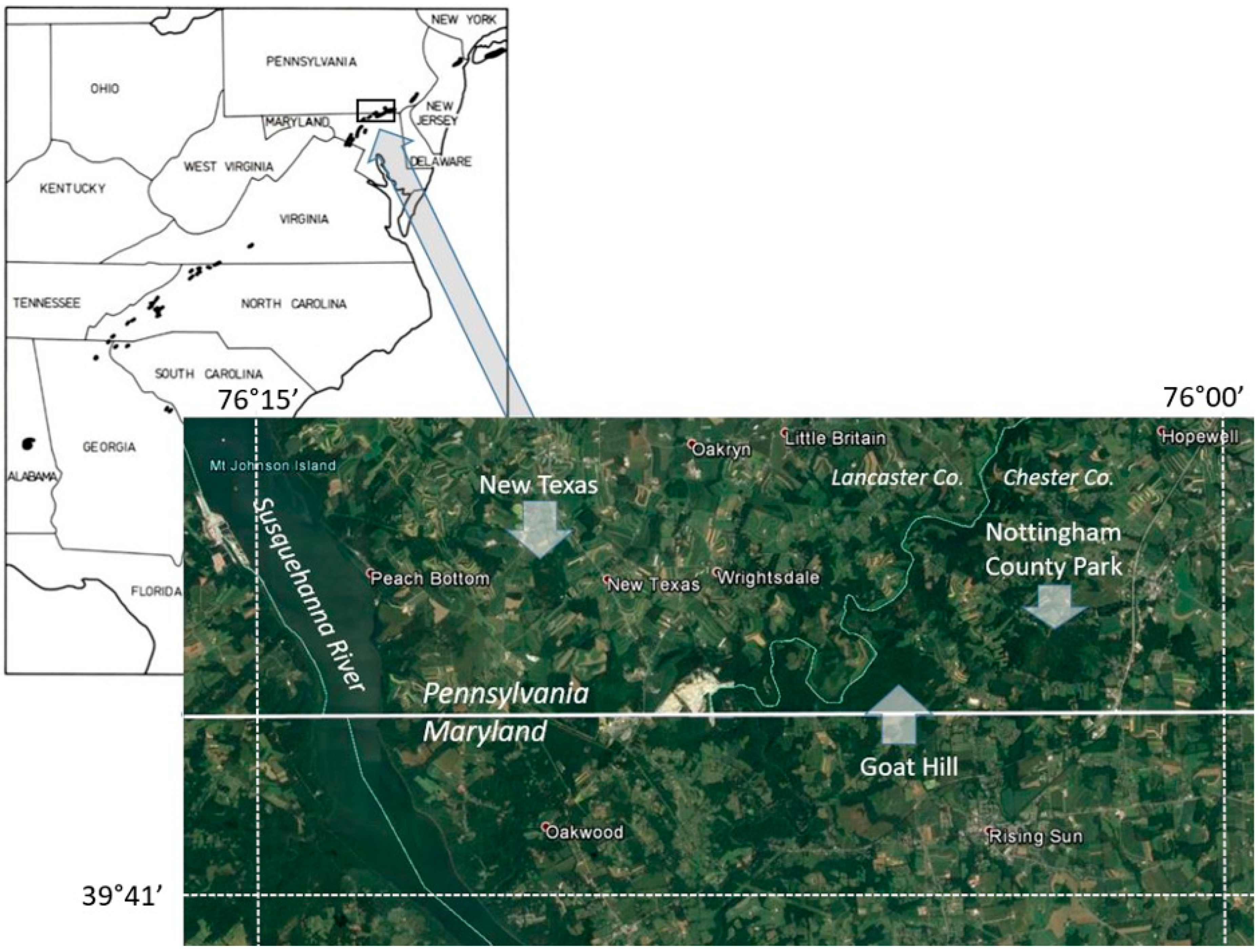
Soil samples were collected from the Goat Hill Barrens, part of the State Line Serpentinite Belt in southwestern Chester County, Pennsylvania (Figure 1). In a weathered and vegetated terrain such as the barrens, soils are a representation, albeit imperfect, of the underlying rock. In addition, the purpose of the original study [33] was to gather material to be used in the study of uncommon sources of soil actinomycetes for the purposes of natural product discoveries. The Goat Hill Barrens are one of the largest areas of a suite of ecological communities known as serpentine barrens: pine-oak forests and open grasslands in the Piedmont and Blue Ridge physiographic provinces of eastern North America with unique species compositions due in part to extraordinarily high Ni and Mg and low Ca in soils weathered from serpentinite [34]. The samples studied here were the coarse fractions (plus 2.5 mm) of two samples from the site. Descriptions of the regional geology, chemistry, bulk mineralogy, palynology and mycology, along with nominal descriptions of the organic petrology of the samples, can be found in Hower et al. [33]. The bulk geochemistry of all samples from the latter work is presented here as Supplemental File S1 Table S1.

2.2. Scanning Electron Microscopy—Energy Dispersive Spectroscopy (SEM-EDS)

Epoxy-bound pellets of samples GH-1 and GH-2 were prepared to a 0.05 μm alumina final polish and sputter-coated with carbon to render the surface conductive. The surface of each was analyzed using a Thermo Fisher/FEI Versa 3D DualBeam scanning electron and focused ion beam microscope (FIB-SEM; Thermo Fisher Scientific, formerly FEI, Hillsboro, OR, USA). The Versa 3D is equipped with a backscatter detector (BSE) to collect atomic number contrast images in which heavy minerals or particles hosting heavy atoms dispersed in a matrix composed of aluminum silicates appear bright. The chemical composition of fly ash particles was determined by energy dispersive X-ray spectroscopy (EDS) using an EDAX Octane Ultra Pro silicon drift detector (EDAX, Pleasanton, CA, USA) solid-state detector mounted on the Versa 3D. The EDS spectra were collected using a voltage of 15 keV to provide sufficient overvoltage to excite most elements (including lanthanides) while retaining a spatial resolution of approximately 1 μm. All SEM-EDS data are listed in Supplemental File S2 Table S2. The SEM images, basic SEM scans, and approximate chemical composition of the scanned spots or areas are in Supplemental Files S3–S5. Note that the detailed information contained in the Supplementary Files is the basic data standing behind the tables and figures in the text.

2.3. Transmission Electron Microscopy (TEM) and Spectroscopy

Based on the SEM-EDS analyses, an area from the epoxy-bound pellet of GH-1 was selected for more thorough analysis. The Versa 3D DualBeam was used to extract and lift out a thin slice, with an approximately 10 μm by 7 μm area, of the promising mineral assemblage. The slice was mounted on a Cu grid and ion milled to approximately 100 nm thickness for analysis with a Thermo Fisher Spectra 300 cold field-emission scanning transmission electron microscope (TEM, also High-resolution TEM or HRTEM; Thermo Fisher Scientific, Hillsboro, OR, USA), operated at 300 keV. TEM images and selected area electron diffraction patterns (SAED) were acquired with a Gatan K3 direct detection camera. Elemental composition and oxidation state at sub-nanometer resolution were collected by Electron Energy Loss Spectroscopy (EELS), using a post-column Gatan GIF BioContinuum HD imaging and energy filter (Gatan, Pleasanton, CA, USA). For EELS acquisition, the TEM was operated in scanning mode, using a C2 aperture of 50 μm, camera length of 600 mm, and entrance aperture of 5 mm, amounting to a convergence semi-angle of 7.4 mrad and a collection semi-angle of 38.3 mrad. Dual EELS spectra [36] were acquired in the low energy range (0–550 eV) and high energy range (500–1050 eV) at a dispersion of 0.1 eV/pixel. In Dual EELS, the two energy ranges are collected in rapid succession to allow removal of any energy shift, evaluation of sample thickness using the low-loss (LL) region in concurrence with the identification and quantification of elements based on their high energy-loss (HL) features. The Gatan Microscopy Suite (GMS) was used to calculate the relative sample thickness, in units of local inelastic mean free path (t/λ), by the log-ratio method [37], for background extraction, using a power-law model, and quantification. Oxidation state of transition elements was estimated from the energy loss near edge structures (ELNES) of the EELS spectra, based on the L3/L2 white-line intensity ratio method according to the procedure described by Van Aken et al. [38] to extract the lines intensity. The relation between white line ratios and oxidation states was empirically derived from standards measured at the same instrument and optics configuration. For a thorough elaboration of the TEM characterization and FIB liftout technique for geologic samples, the reader is referred to Stroud and Singerling [39]. The EDS scans of areas of interest were examined by plotting the data with SigmaPlot version 15 (Grafiti LLC, Palo Alto, CA, USA) and selecting energy (eV) and count ranges for enhancement. Mineralogical identification of grains was based on chemical composition and crystal structure data obtained from SAED and HRTEM. The same GMS image analysis software (version 3.6) used to analyze the EELS spectra was also used to measure crystal structure parameters from SAED and HRTEM. For HRTEM images, lattice spacing and angles were measured from the corresponding fast Fourier transform (FFT).

3. Results and Discussion

3.1. Previous Study

Based on X-ray diffraction analysis, the relative abundances of minerals in the coarse and fine (soil) fractions of the samples were determined by Hower et al. [33]. As shown in

Table 1. Relative abundances of minerals from Goat Hill samples 1 and 2 [33].

GH-1 coarse	lizardite +/− antigorite >> clinochlore (?) > quartz, chrysotile, chromite (?)
GH-1 soil	lizardite +/− antigorite >> quartz > clinochlore (?) > chromite (?) > chrysotile > biotite
GH-2 coarse	lizardite +/− antigorite > dolomite > clinochlore (?) > chromite (?), quartz > talc
GH-2 soil	lizardite +/− antigorite > quartz (?), clinochlore (?) > chromite (?) > talc, chrysotile, dolomite, diopside (?)

, lizardite (Triclinic; Mg₃Si₂O₅(OH)₄) and antigorite (Monoclinic; (Mg, Fe)₃Si₂O₅(OH)₄) are the most abundant minerals, with chrysotile, the monoclinic Mg₃Si₂O₅(OH)₄ mineral, having a lower abundance. Lizardite is an end member of the Lizardite-Népouite (Ni₃Si₂O₅(OH)₄) series (https://www.mindat.org/min-2425.html; accessed on 23 January 2026), an important consideration with respect to the relative abundance of Ni in certain samples. Along with clinochlore (Mg, Fe⁺⁺)₅Al(Si₃Al)O₁₀(OH)₈), dolomite (CaMg(CO₃)₂), talc (Mg₃Si₄O₁₀(OH)₂), diopside (MgCaSi₂O₆), and biotite (K(Mg,Fe)₃AlSi₃O₁₀(F,OH)₂), the predominance of MgO among the major oxides is justified. As noted above, along with the chromite (with the Wood Mine in Lancaster County being the world’s largest source from 1827 to 1882 [29,30,32]; https://www.mindat.org/loc-4086.html, accessed on 30 June 2025), talc, and asbestos production from the region [30], the Goat Hill mine was the primary producer of magnesia in the U.S. from 1835 to 1860 [https://www.mindat.org/loc-15169.html, accessed on 30 June 2025].

3.2. SEM-EDS Studies

3.2.1. Spinel Minerals

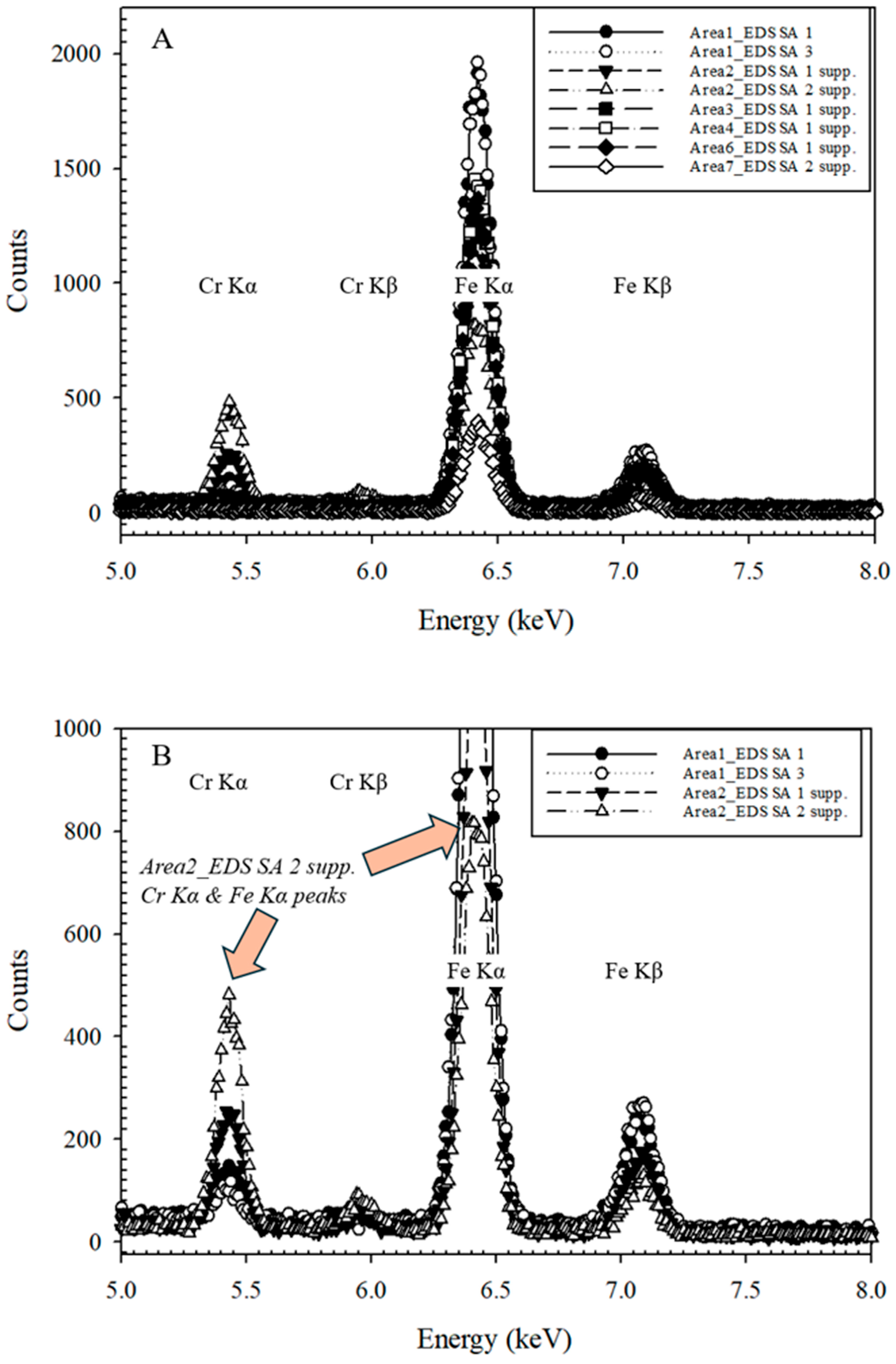
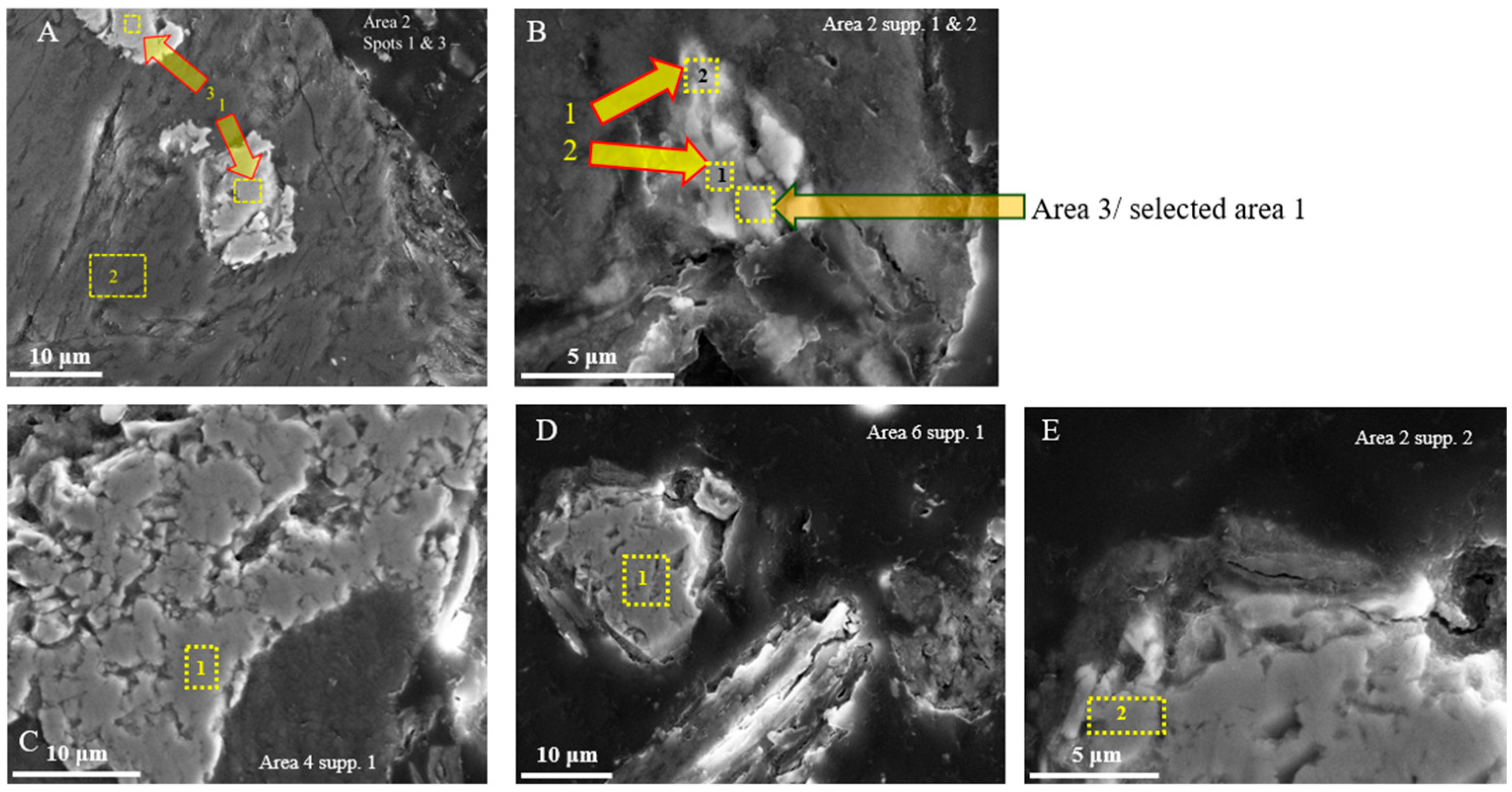
The presence of Fe- and Fe-Cr spinels in GH-1 is noted in Figure 2, with Figure 2A,B showing Fe-Cr spinels and Figure 2B (area 3/selected area 1) and Figure 2C–E showing Fe-spinels (magnetite). The distinction between the spinel forms is accomplished via the identification of the Cr and Fe Kα and Kβ peaks within the 5.0–8.0 keV energy range (Figure 3A). All of the grains examined in Figure 3A have distinct Fe peaks, but only four of them have significant Cr peaks (Figure 3B). Of those four grains, the “Area2_EDS SA 2 supp.” scan shows a mineral approaching the ideal composition of chromite (Fe⁺⁺Cr₂O₄). While the “Counts” axis is not a precise measure of the relative concentration, note that the Cr Kα peak of ca. 500 counts vs. the Fe Kα of ca. 800 counts falls short of the expected 2:1 Cr:Fe ratio. The scanned EDS area, though, represents a measurement from a volume, not just the area indicated, so a mix of chromite and magnetite, or other minerals, could be contributing to the EDS scan. Exsolution of spinel minerals was not observed.

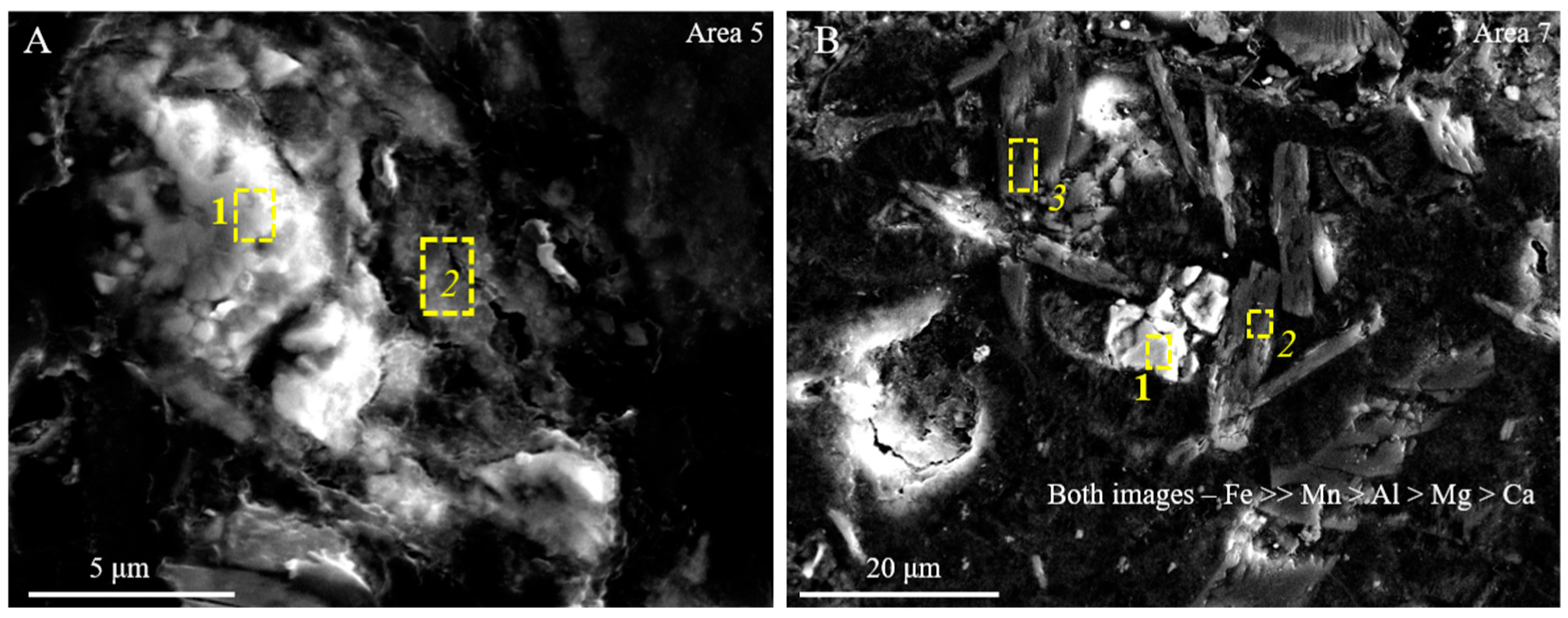
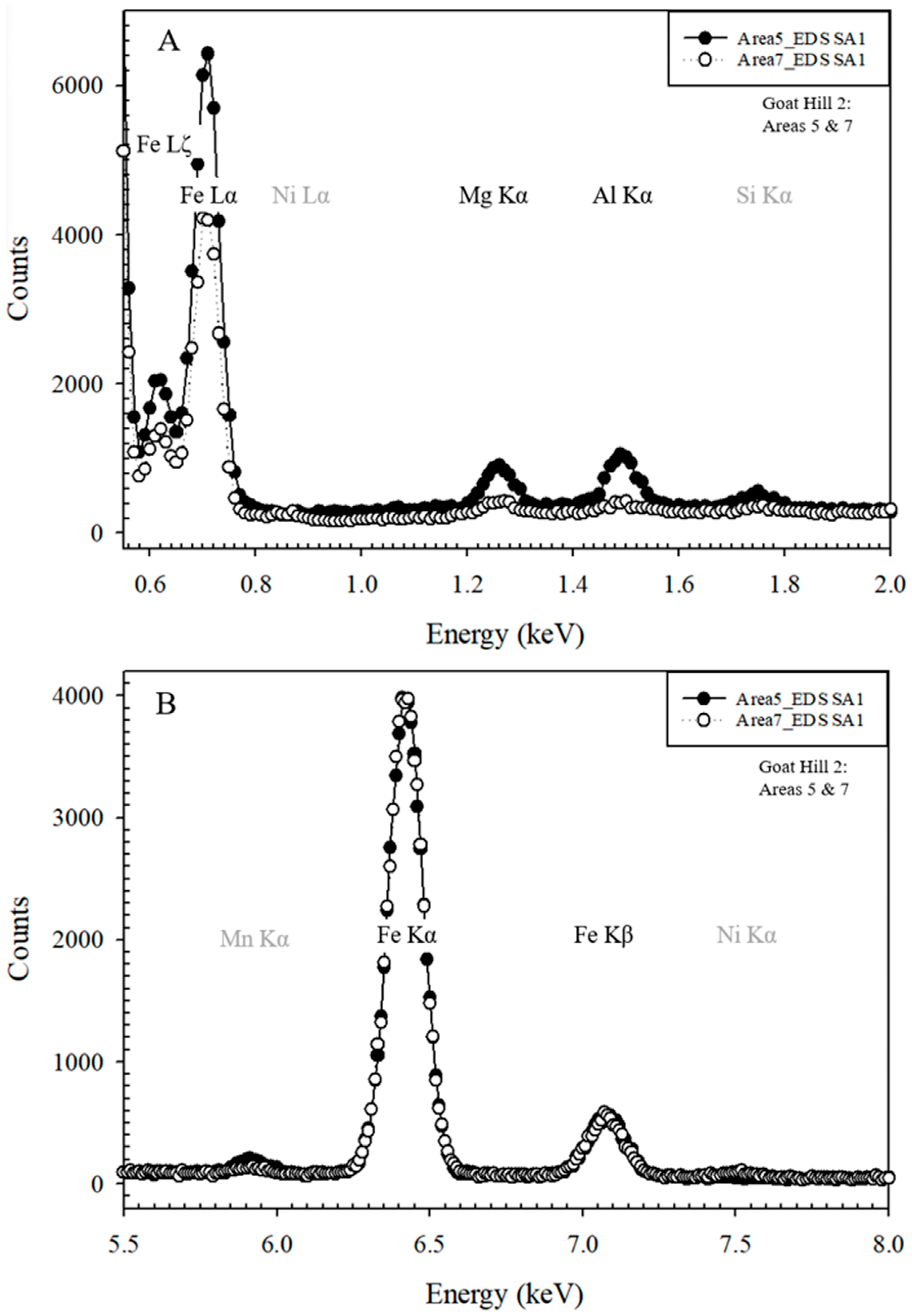
Goat Hill site 2, area 5, selected area 1 (Figure 4A) and area 7, selected area 1 (Figure 4B) also contain Fe-spinel minerals. The EDS scans for 0.55–2.0 keV (Figure 5A) and 5.5–8.0 keV (Figure 5B) suggest that the mineral is magnetite. While Mg, Al, Mn, and Ni could be present in the spinel structure, it is also possible that those elements, along with the Si, are from the area surrounding the spinel.

For further discussions of chromite and other spinel minerals, see Palache et al. [40], Picot and Johan [41], and Ramdohr [42].

3.2.2. Al >> Mg > Ca Mineral

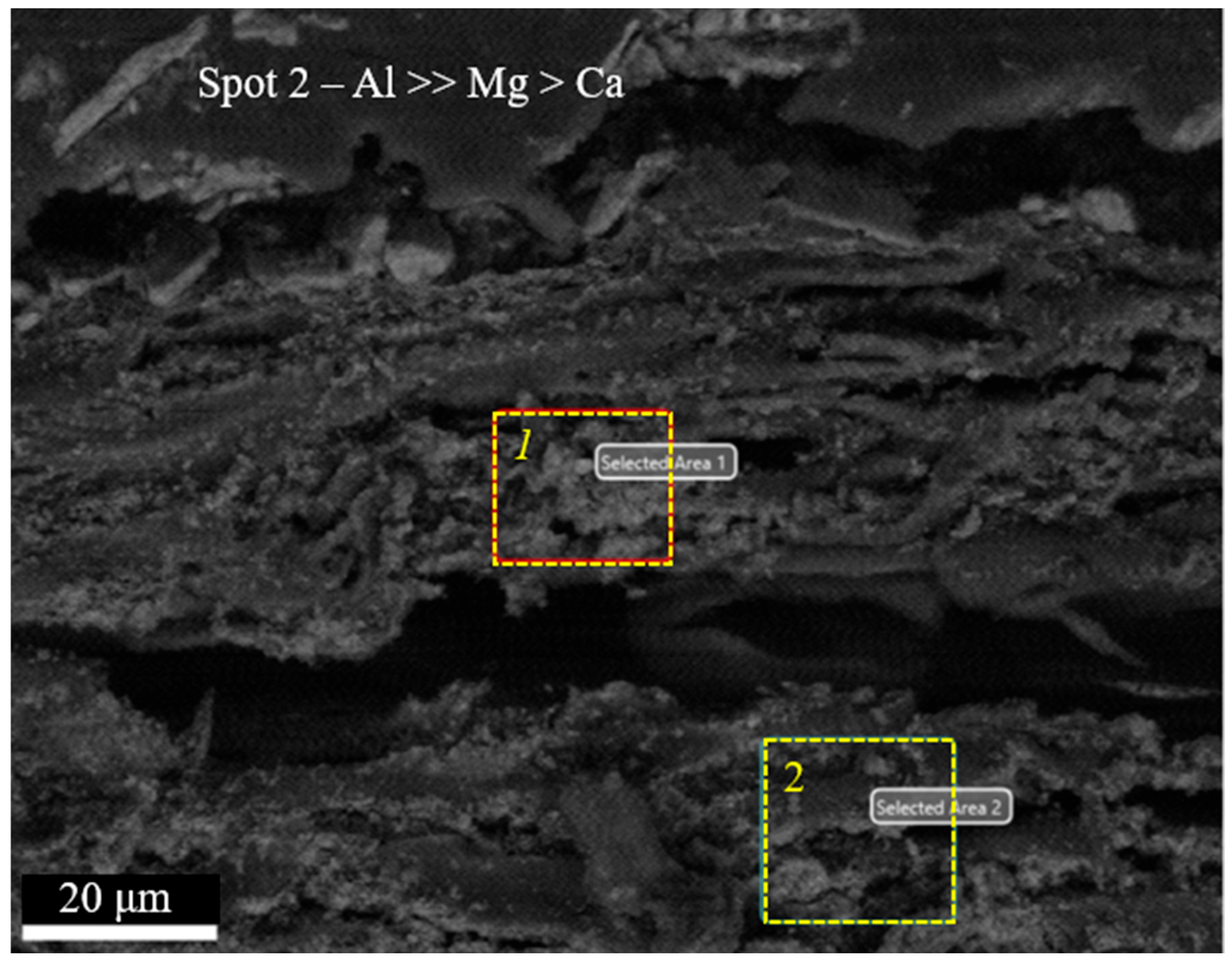
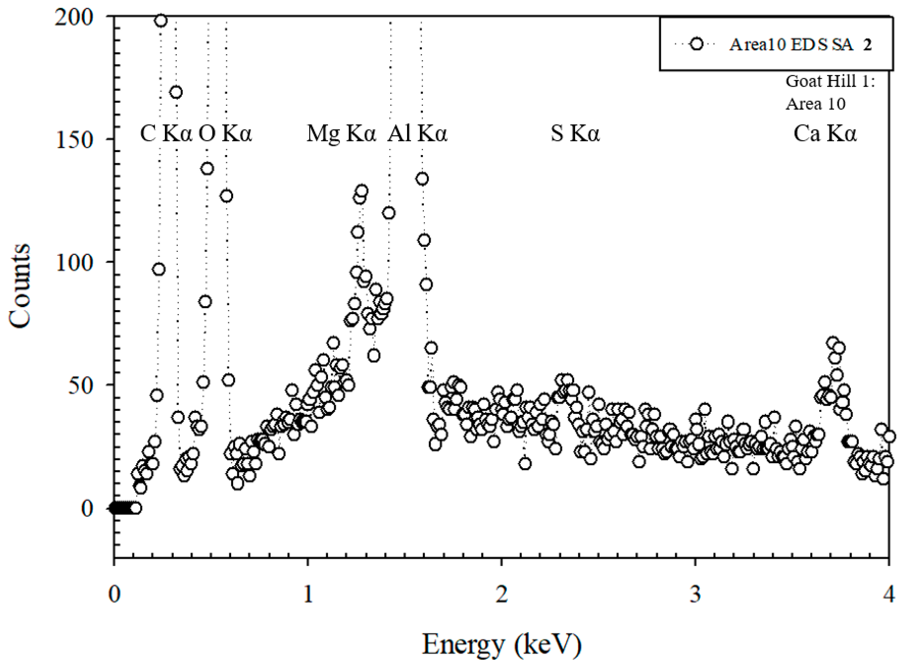
Goat Hill site 1, area 10, selected area 2 (Figure 6) is dominated by the chlorite mineral clinochlore (Figure 7). The mineral is dominated by Al and Mg, with the exclusion of Fe and Si, and the substitution of Ca in the structure.

3.2.3. Various Minerals in Goat Hill Site 1 Area 3

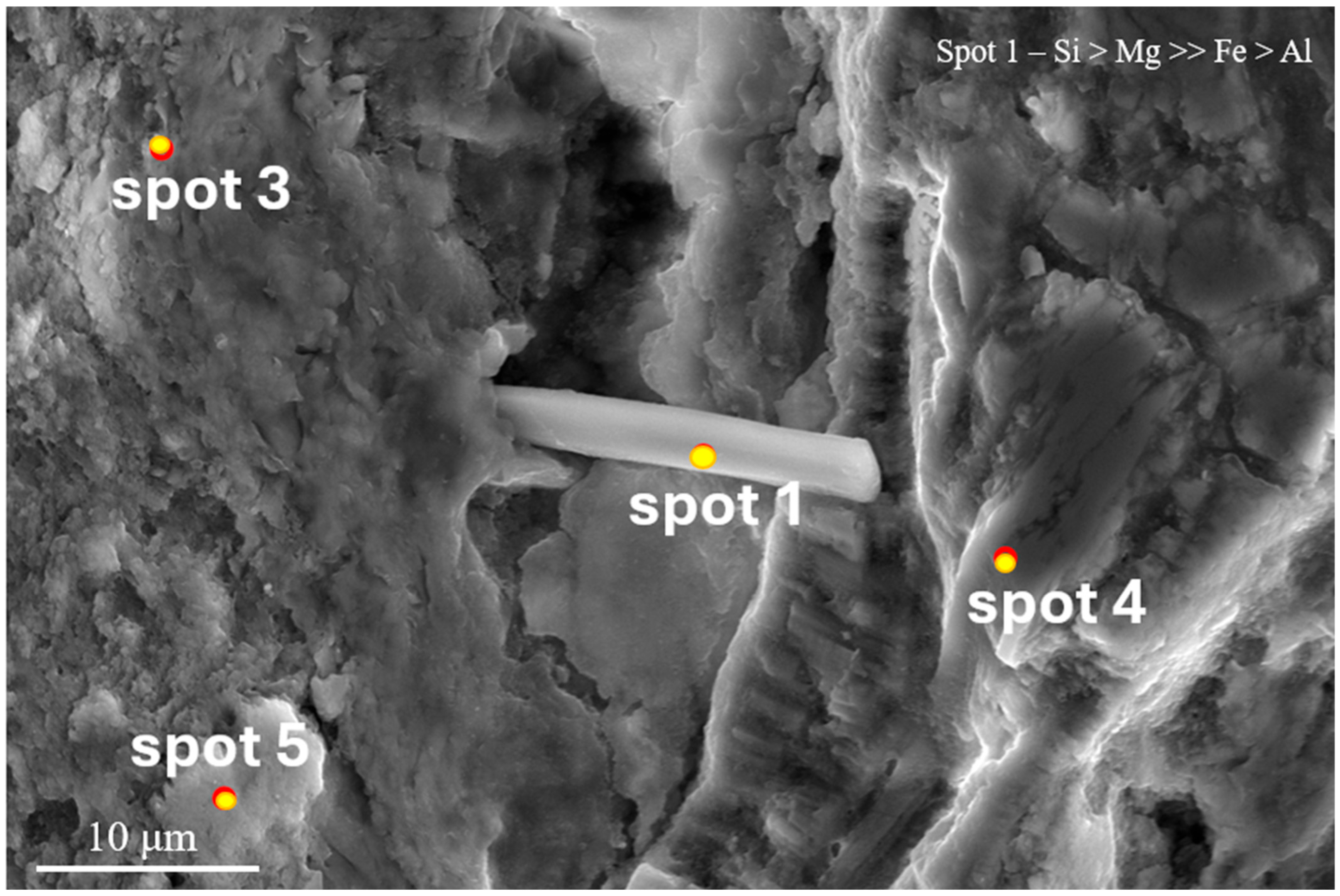
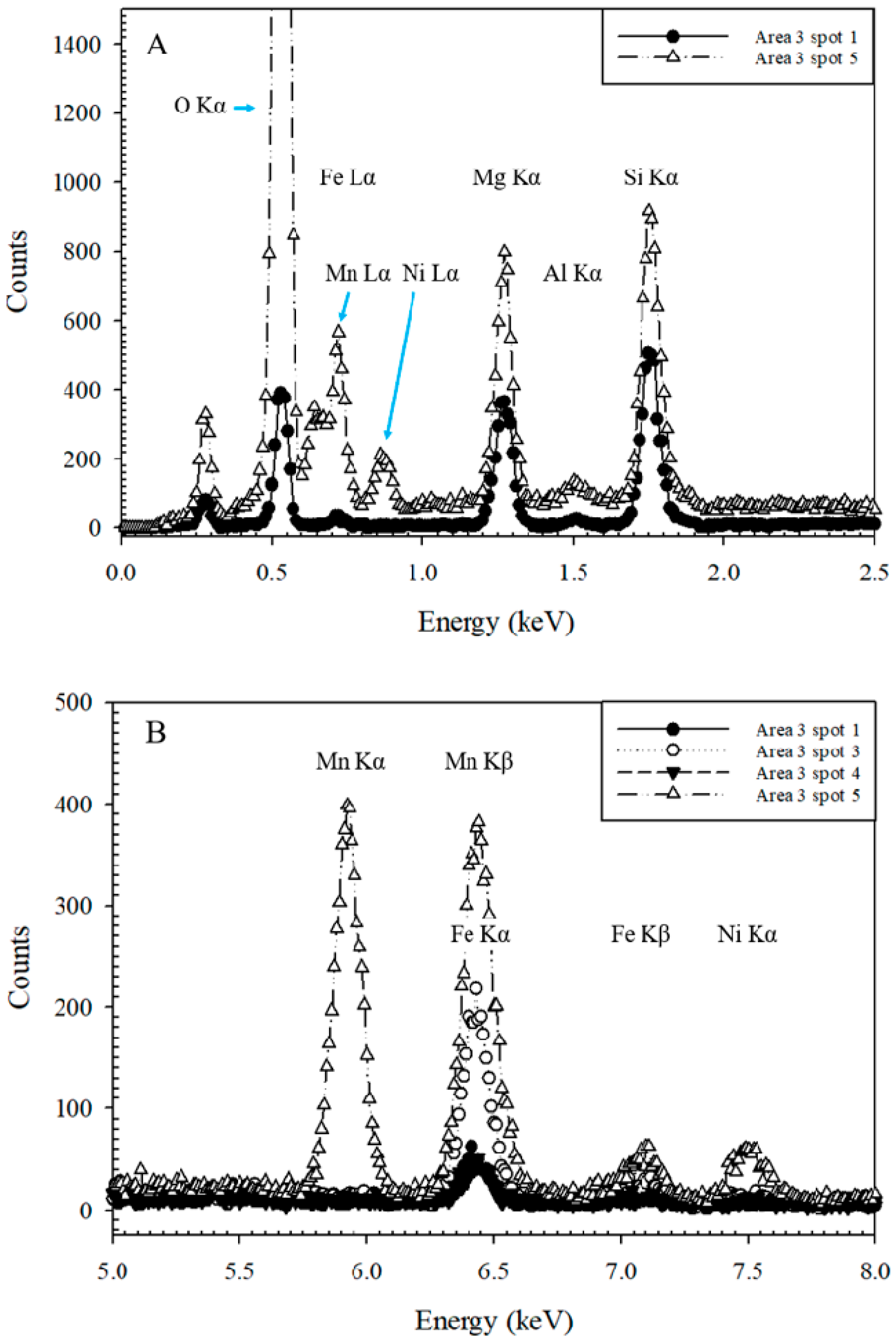
Goat Hill site 1, area 3, spot 1 is a rod-like mineral (Figure 8) dominated by Si and Mg with minor Fe (Figure 9A,B). Based on the Si-Mg chemistry and the confirmation by HRTEM, the mineral is identified as antigorite. Spot 5 is a Si > Mg > Mn >> Fe ≈ Ni > Al mineral in the lizardite subgroup of serpentine minerals (Figure 8 and Figure 9).

3.2.4. Zn-Al Mineral

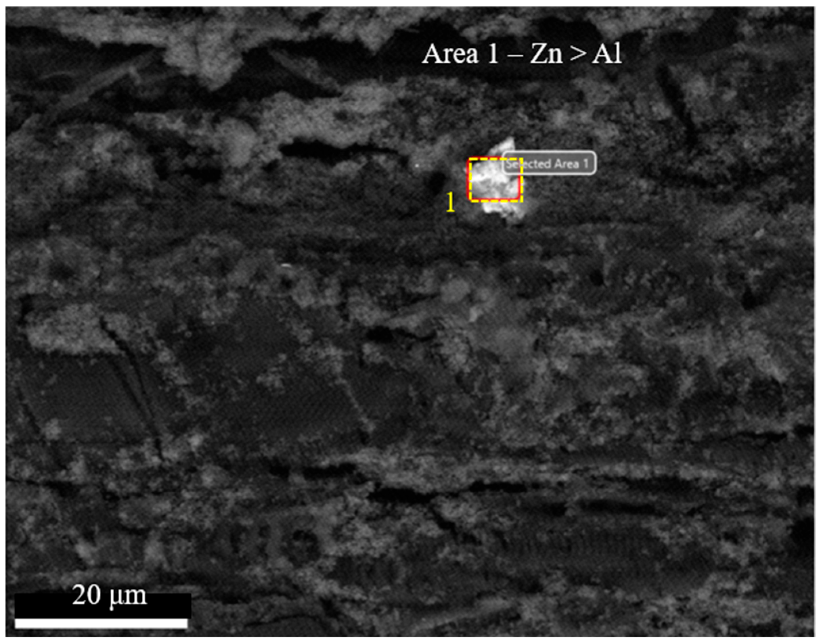
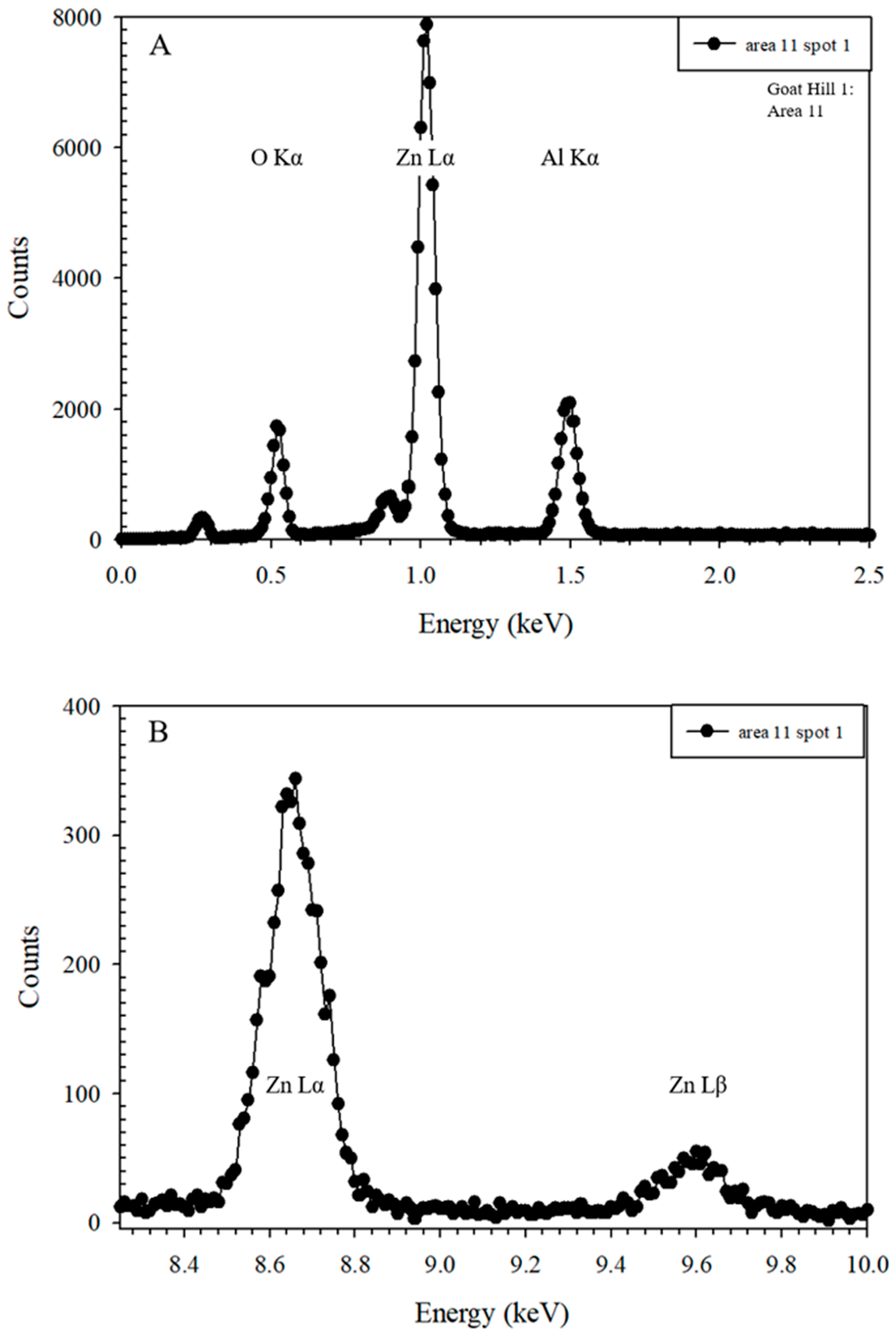
The Goat Hill site 1, area 11, spot 1 (Figure 10), dominated by Zn and Al (Figure 11A,B), is identified as gahnite (ZnAl₂O₄), an Al-group spinel mineral, based on the chemistry and the spinel-like shape of the mineral [40].

3.2.5. Goat Hill Site 1 Area 7 Mg ≈ Si Minerals

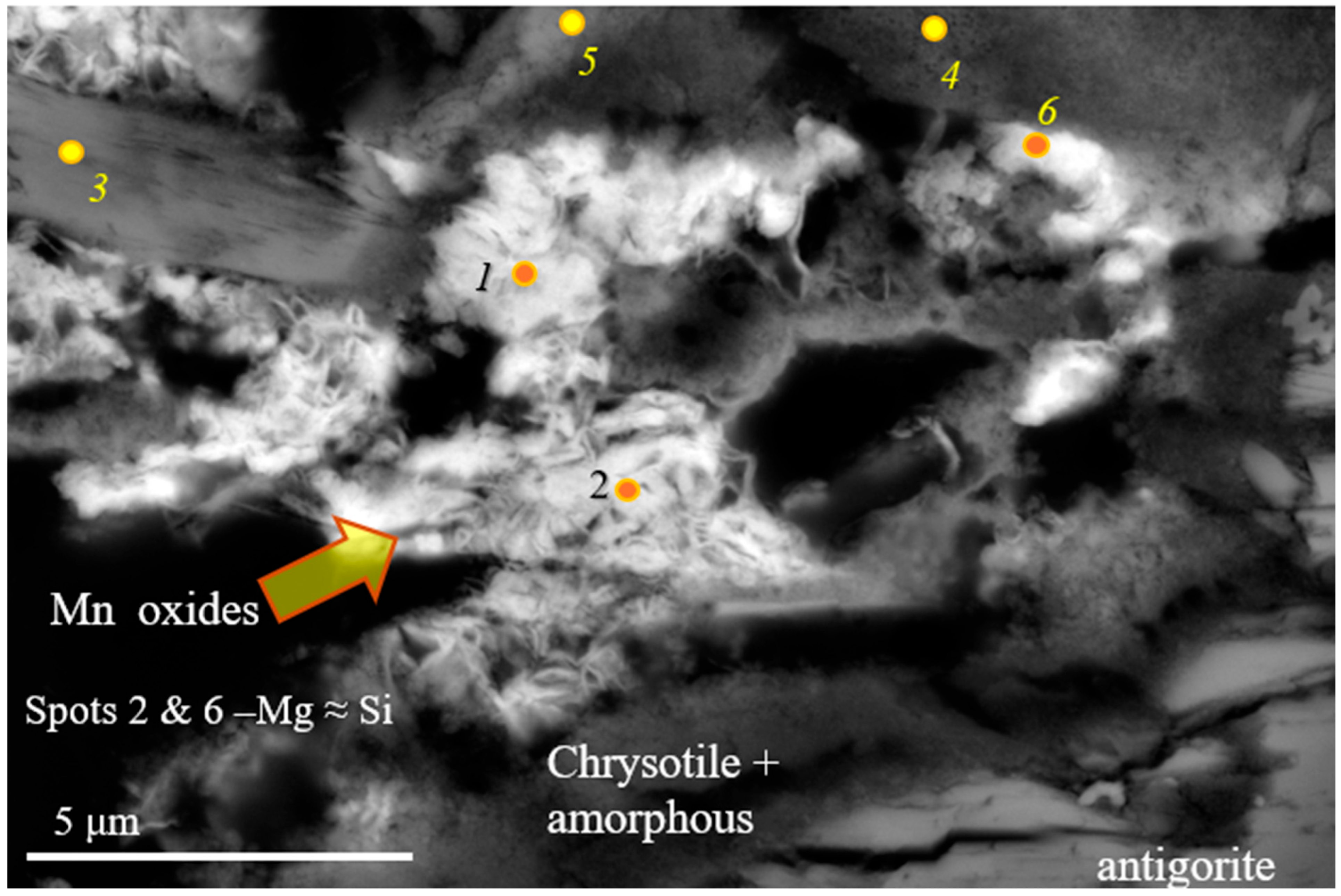
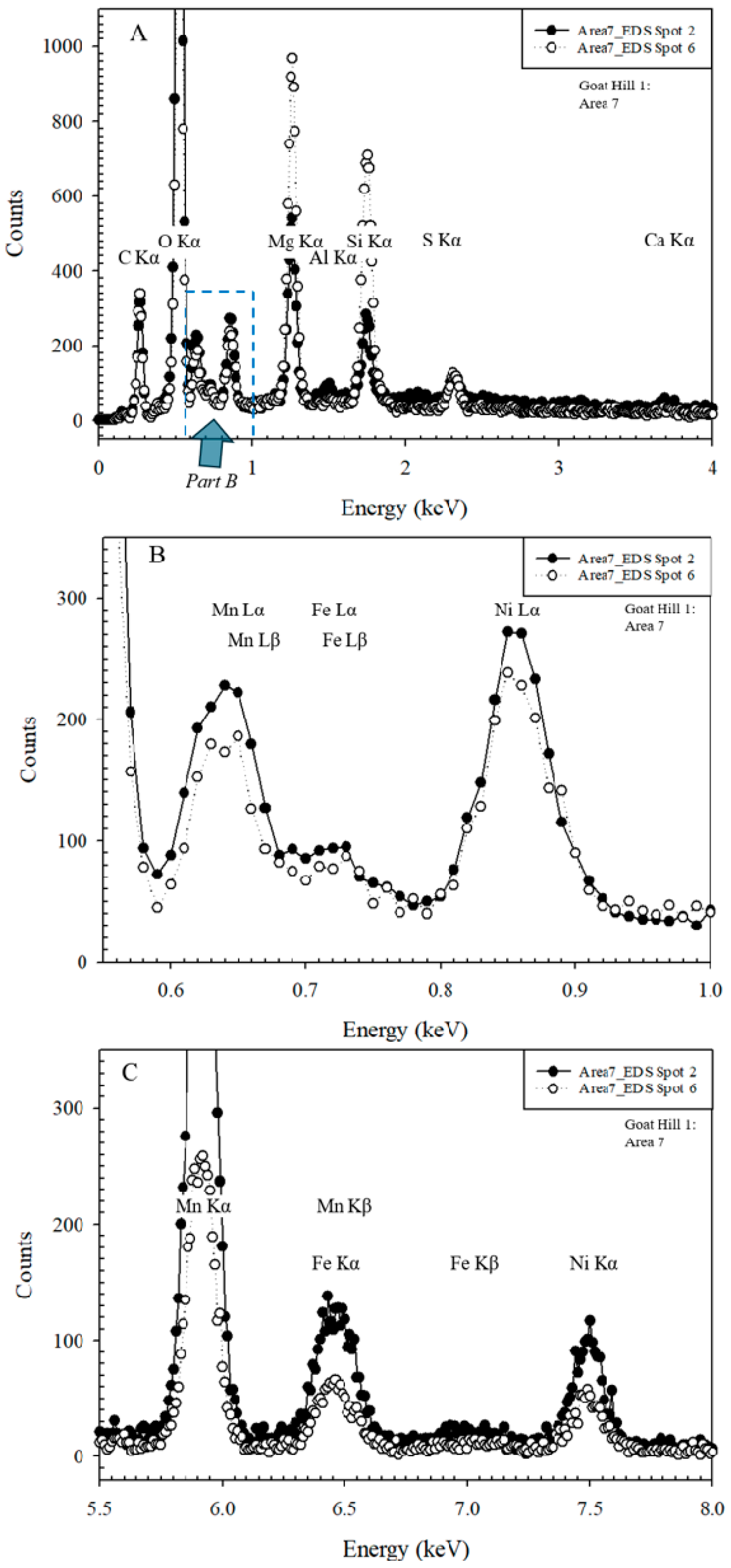
Goat Hill site 1, area 7, spots 2 and 6 (Figure 12) have significant Mg and Si EDS peaks (Figure 13A), minor amounts of Mn and Ni (Figure 13B,C), lesser concentrations of S and Ca (Figure 13A), and insignificant amounts of Fe (Figure 13B,C). The Mg and Si concentrations suggest that the mineral could be lizardite. Other lizardite group minerals contain Mn and Ni (respectively, caryopilite and népouite); however, based on the HRTEM and EELS studies, discussed below, the Mn is in separate Mn oxides. For both spots in this view, Mg >> Ni > Mn > Fe. The assessment of Ni having a higher concentration than Fe is based on the respective Lα peaks. The estimate could be confounded by the evaluations of the Kα peaks, but it is likely that the proximity of the Mn Kβ and the Fe Kα peaks leads to an overestimate of the Fe Kα peak.

3.2.6. Goat Hill Site 1 Area 12 Spots 1, 2, and 3

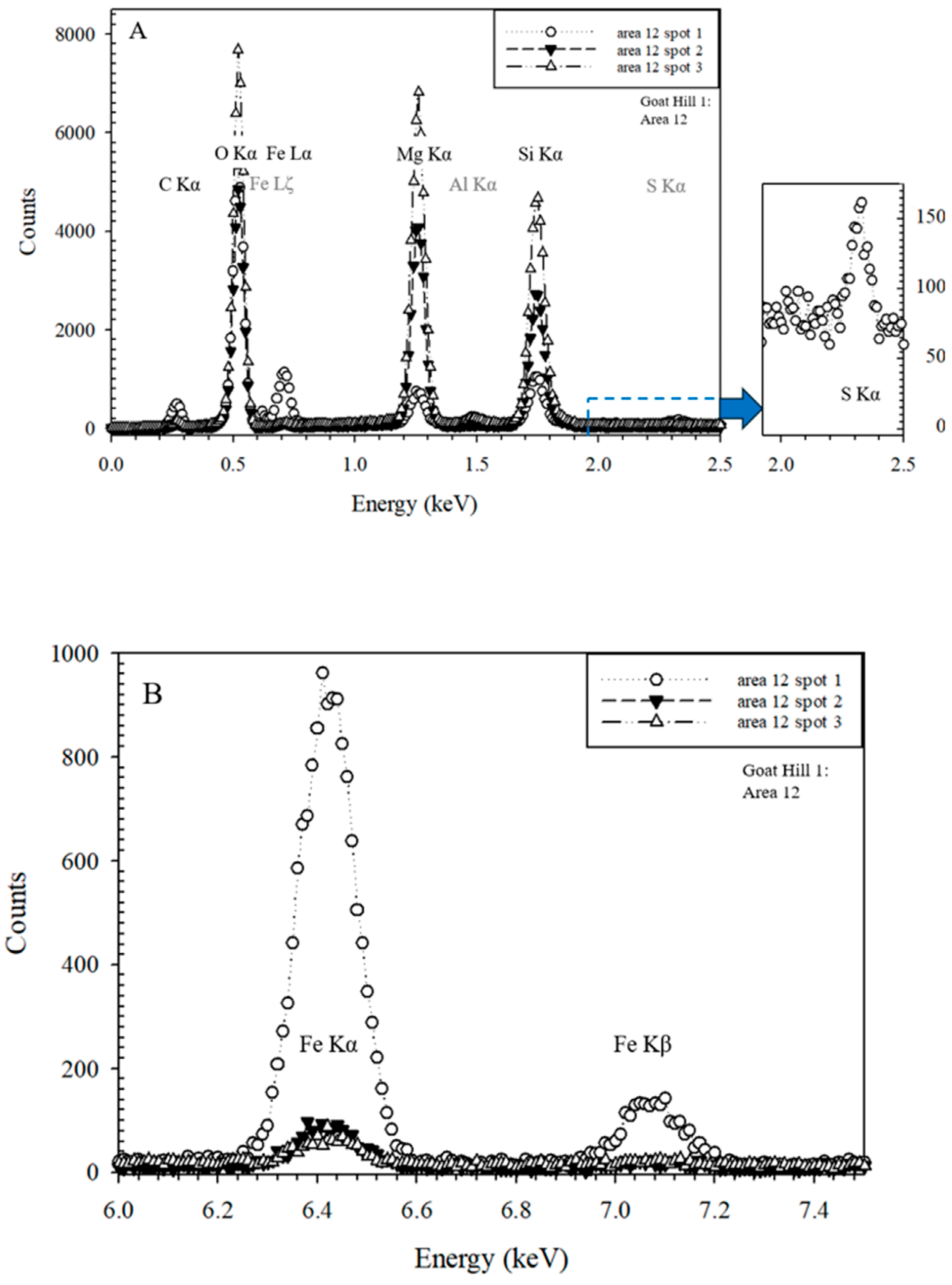
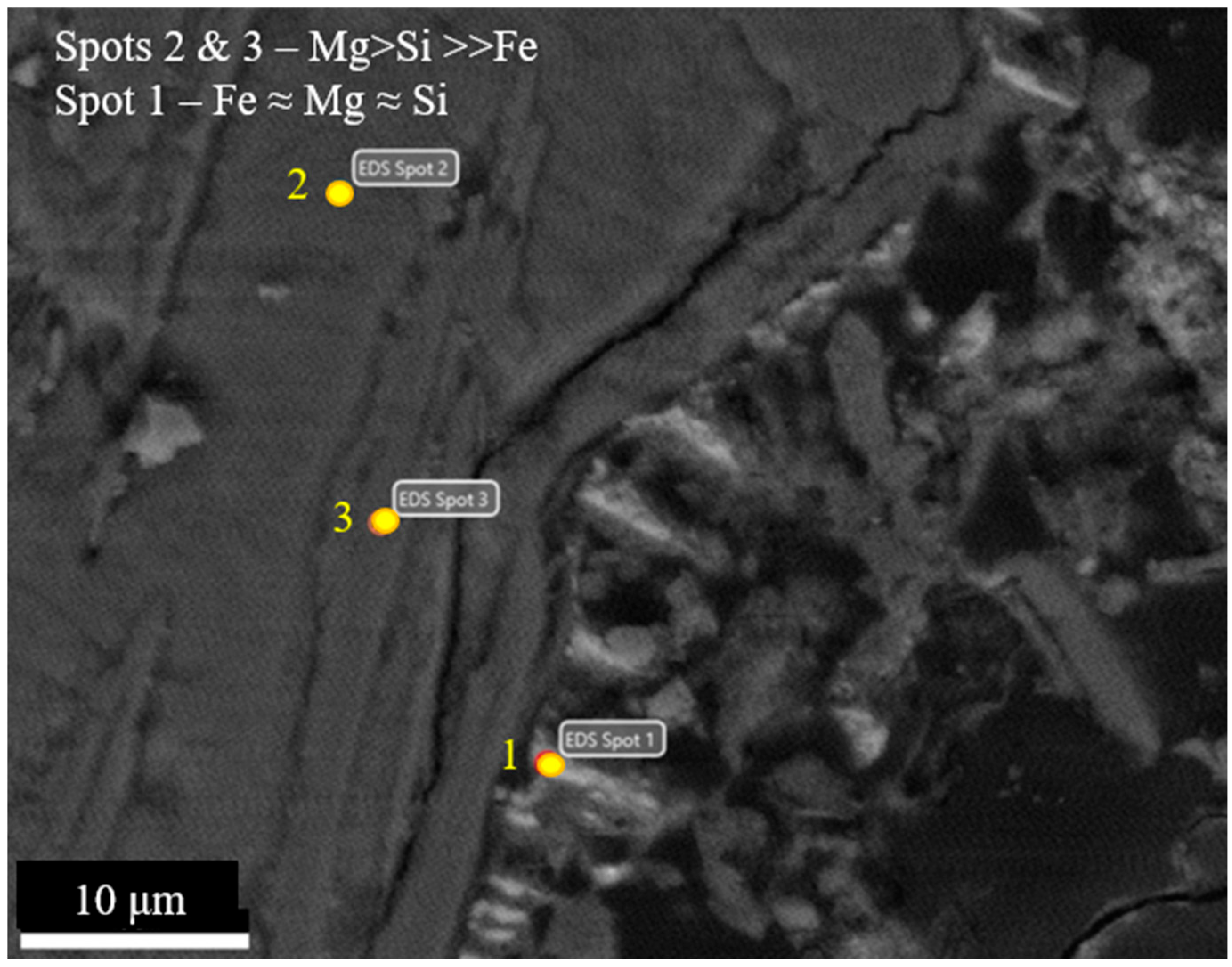
Goat Hill site 1, area 12, spots 2 and 3, similar to minerals discussed in Section 3.2.3 (spot 5) and Section 3.2.5 (spots 2 and 6), are lizardites (Figure 14 and Figure 15). The spot 1 mineral is a blade-like form (Figure 14) with a chemistry dominated by Mg ≈ Si >> S; based on the HRTEM examination, the mineral is identified as antigorite. The source of the S is not known.

3.3. TEM-Based Studies

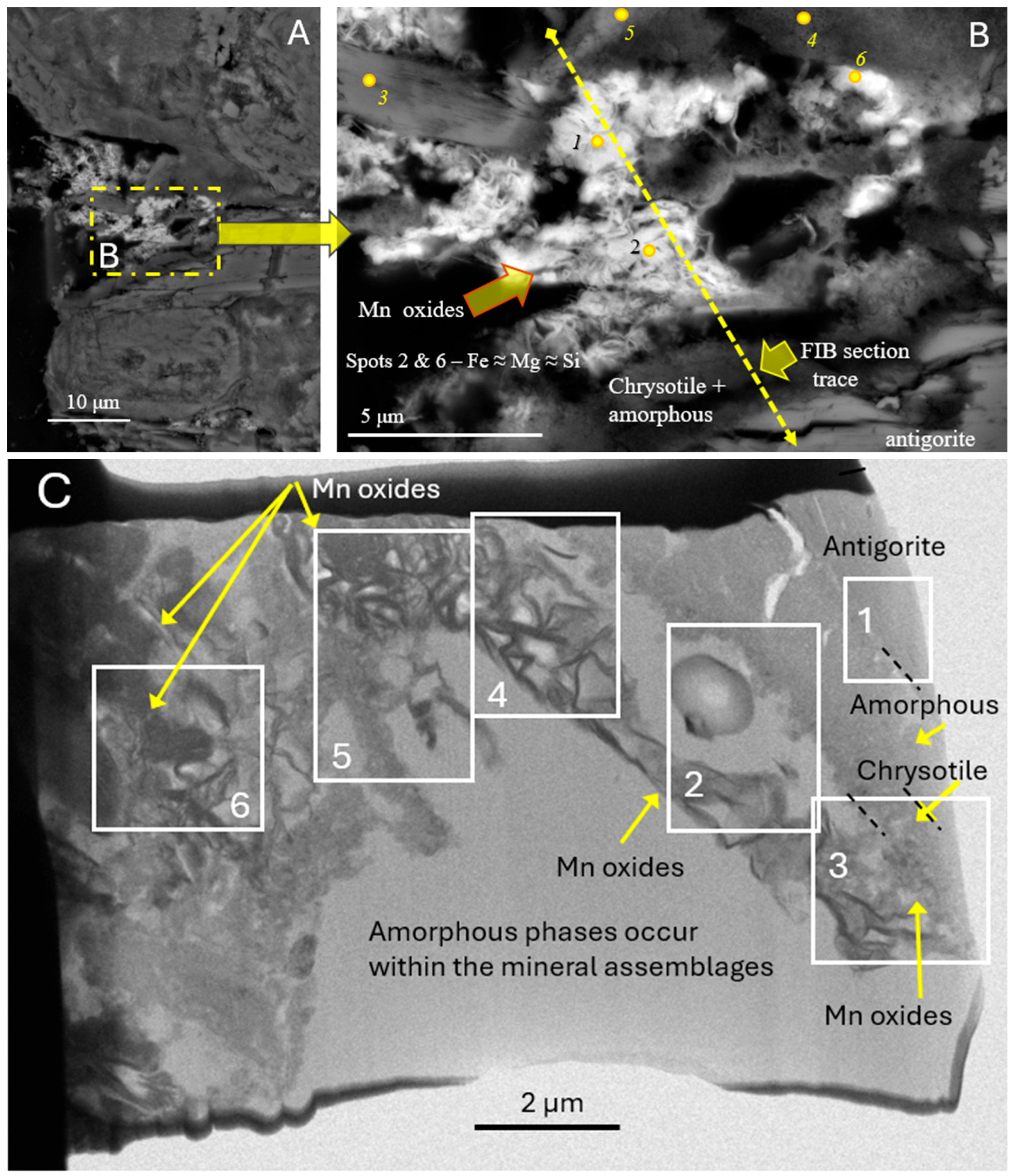
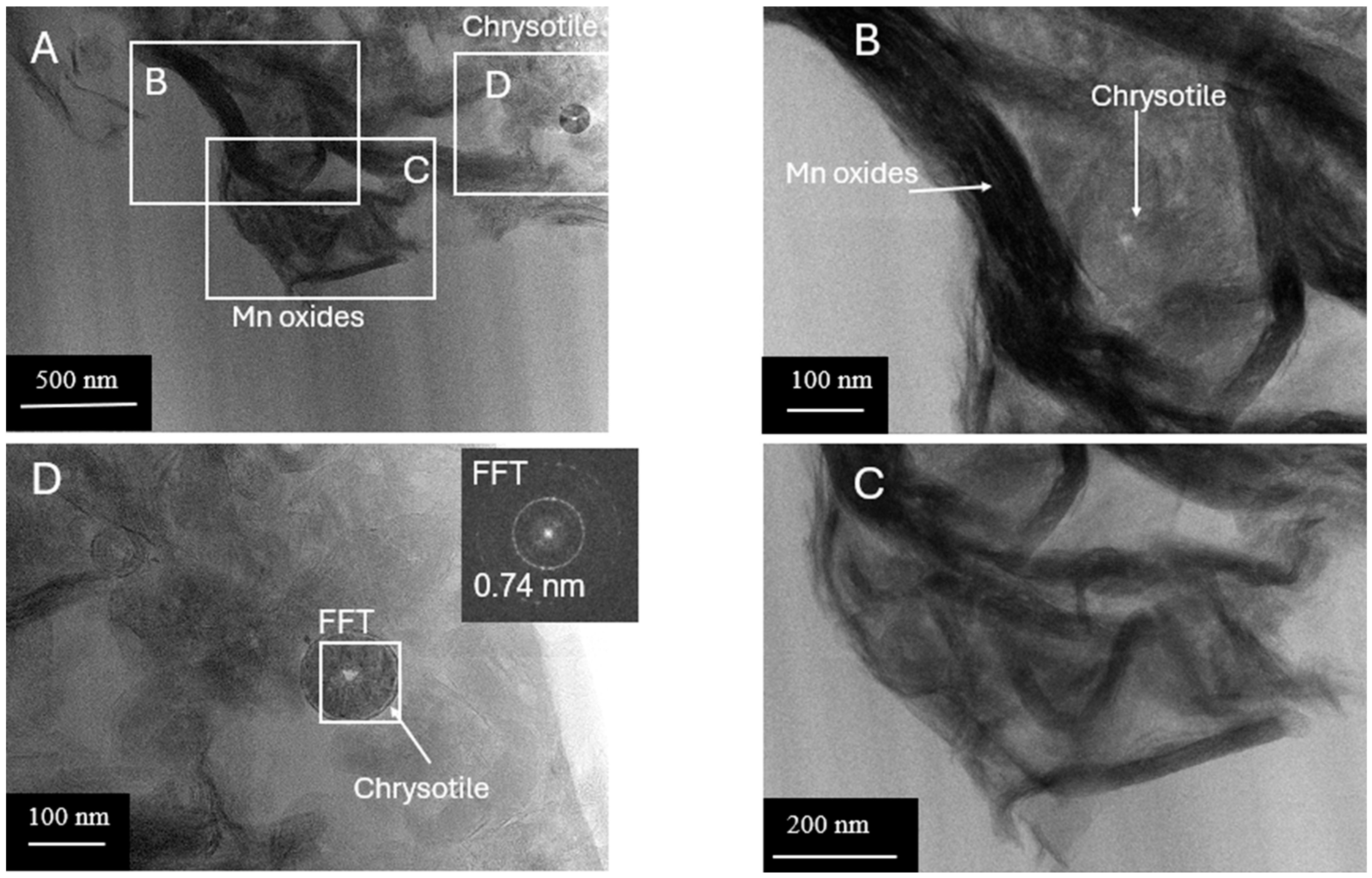
The area discussed in Section 3.2.6 was selected for TEM examination owing to the presence of Mn oxides, chrysotile, antigorite, and amorphous phases (Figure 16A,B). The location of the FIB section trace is shown in Figure 16B, and the back-scatter image of the FIB section, along with the map of the six detailed areas discussed below in connection with Figure 17, Figure 18, Figure 19, Figure 20, Figure 21, Figure 22, Figure 23, Figure 24, Figure 25 and Figure 26.

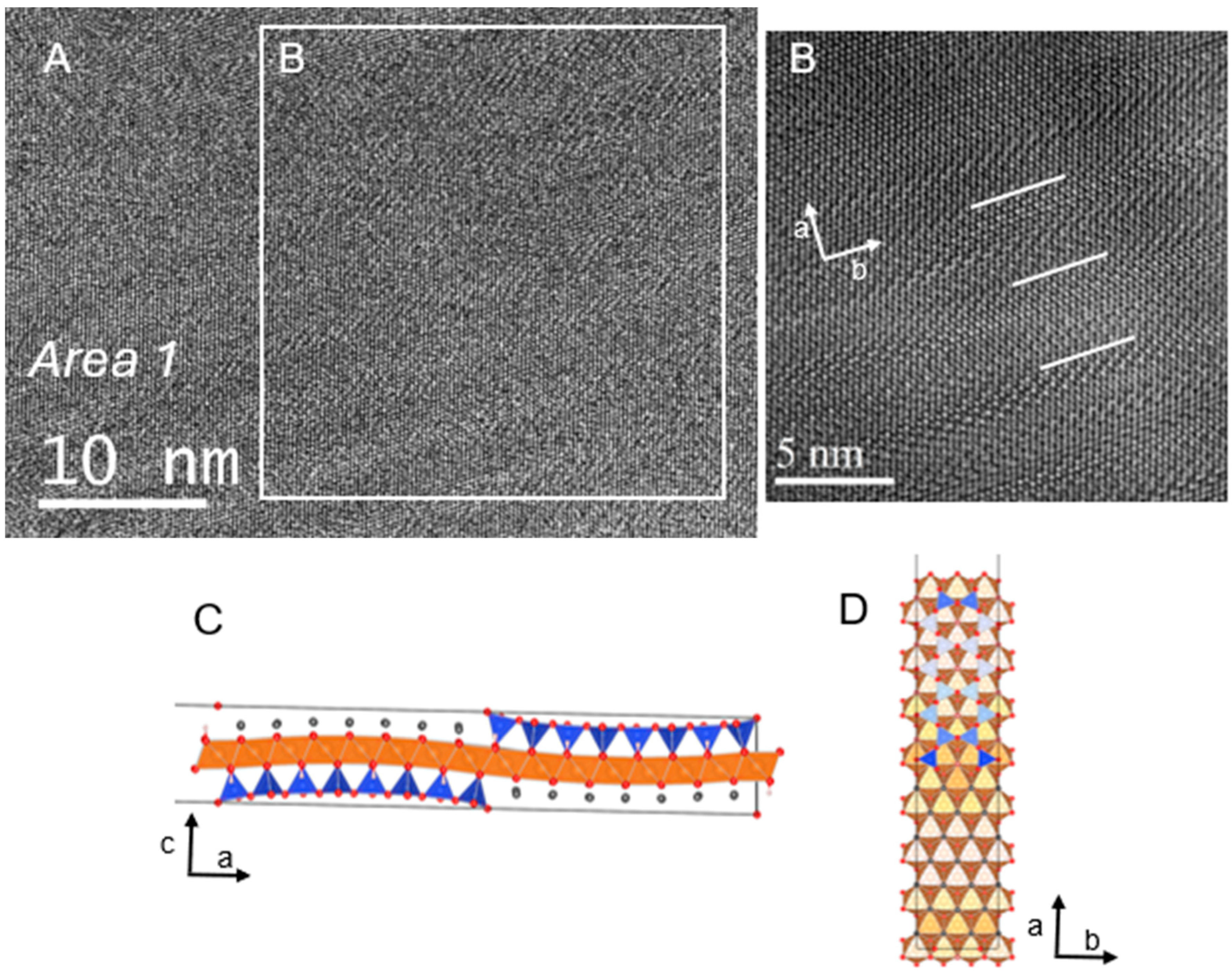
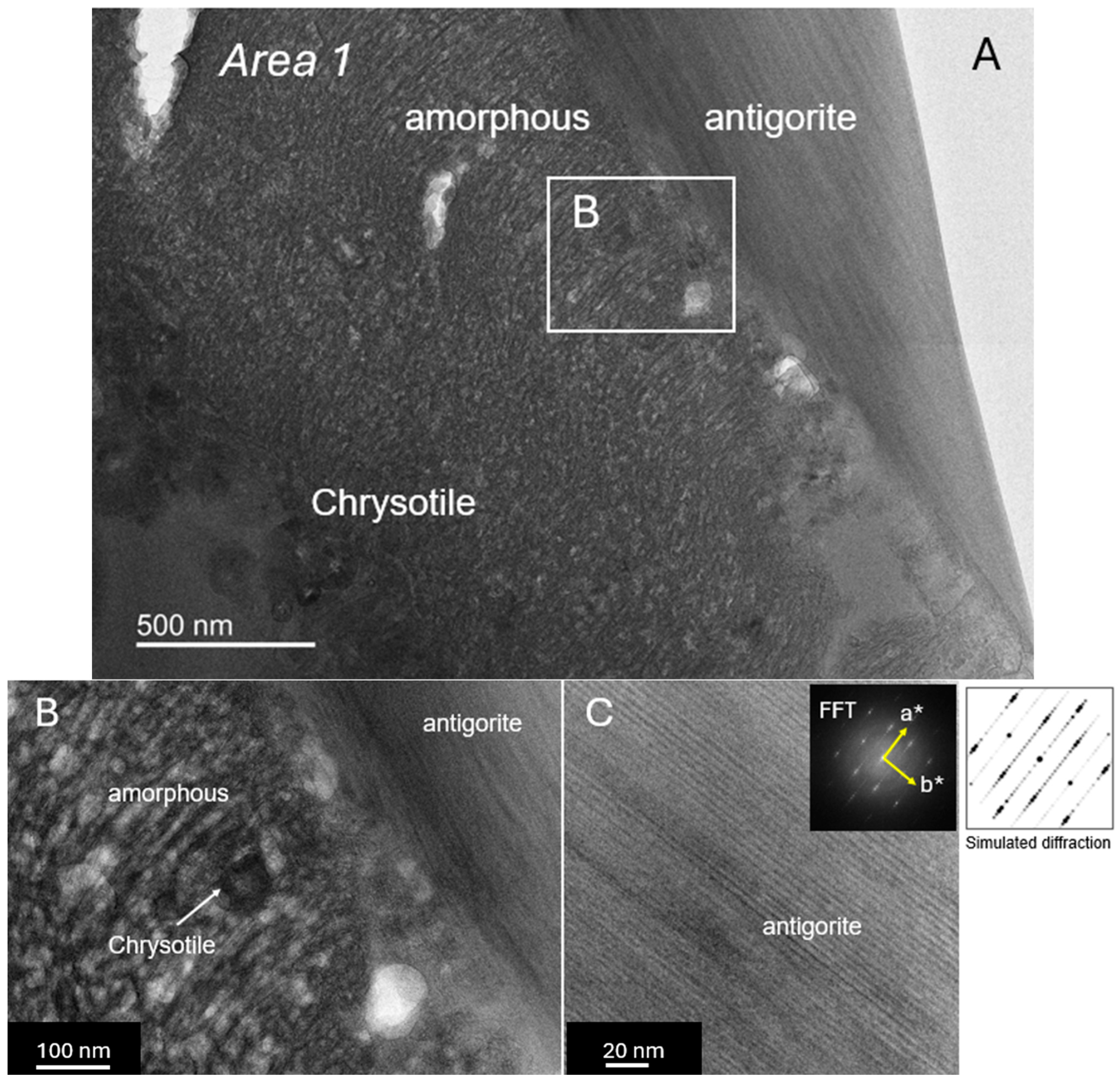
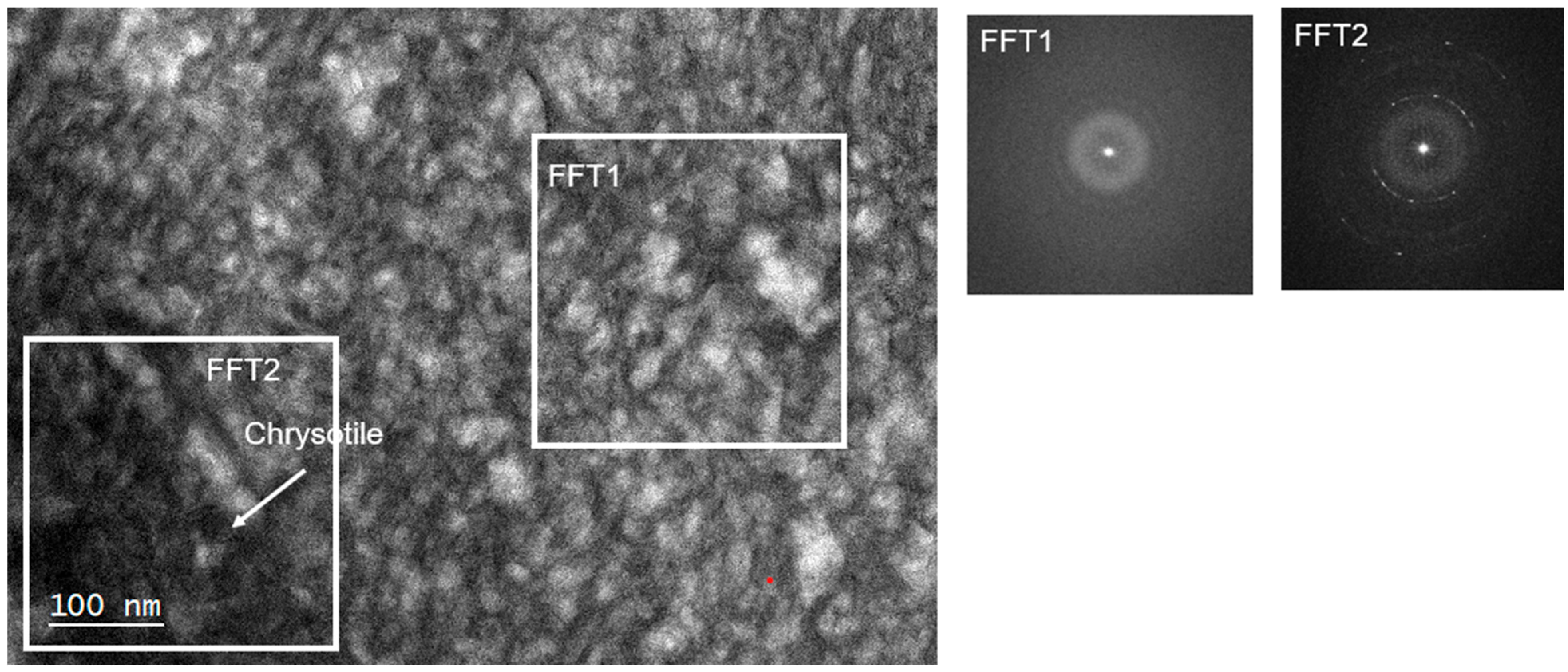
Area 1 consists of chrysotile, antigorite, and amorphous phases (Figure 17A). With respect to the amorphous phases, they could represent a relatively recent alteration resulting from the interaction between serpentine and groundwater, potentially facilitated by microbial activity. There was a clear spatial transition from chrysotile to amorphous phase, including isolated chrysotile fibers mixed with the amorphous phase. In cross-section, chrysotile is seen as a rounded fiber (Figure 17B). Fast Fourier transform (FFT) analysis confirmed the identification of antigorite (Figure 17C). Antigorite (Figure 18A) shows periodic contrast reversal of the SiO₂ tetrahedra as seen in the subtle patterns in Figure 18B. The projections of the inversions on the 010 and 001 planes are shown in Figure 18C and Figure 18D, respectively. The scale of antigorite modulation ranges between 3.3 nm and 110 nm [43]. For the antigorite examined in this section, the modulation is ~3.3 nm. The antigorite is rimmed by an amorphous phase containing sparse chrysotile fibers, which become more abundant with increasing distance from the antigorite. The diffraction contrast between amorphous phases and chrysotile is emphasized in the FFT1 and FFT2 patterns, respectively (Figure 19).

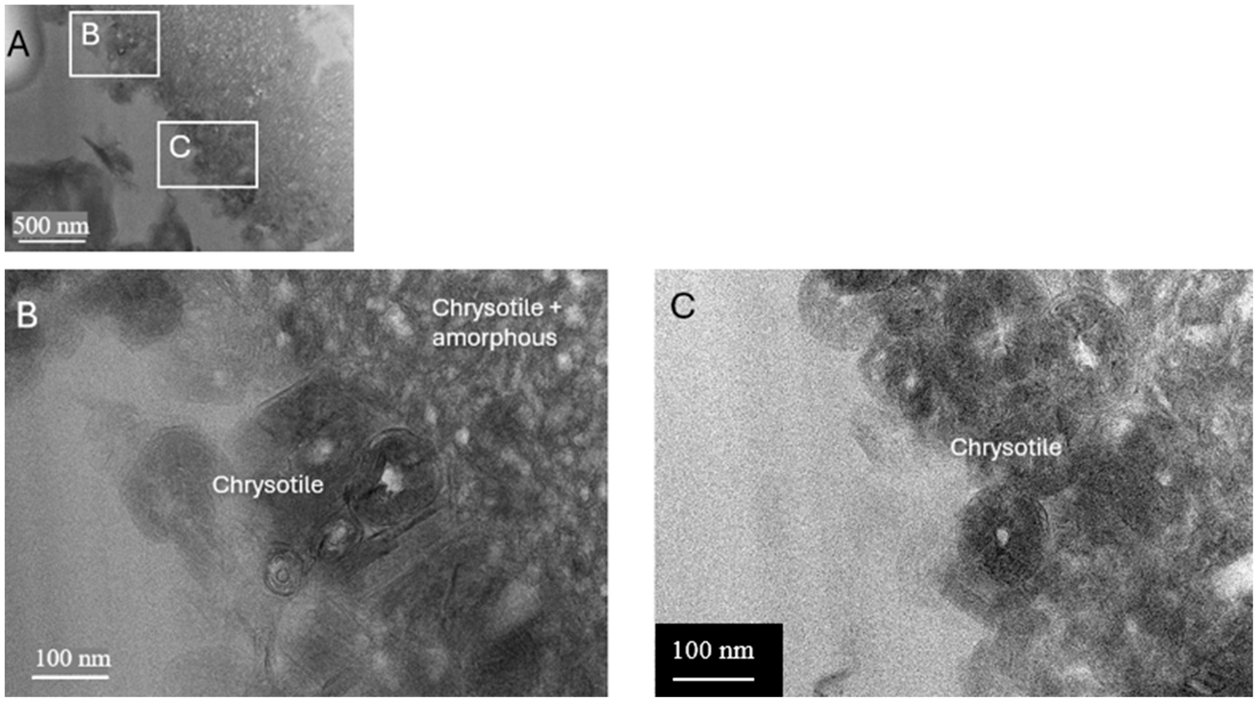
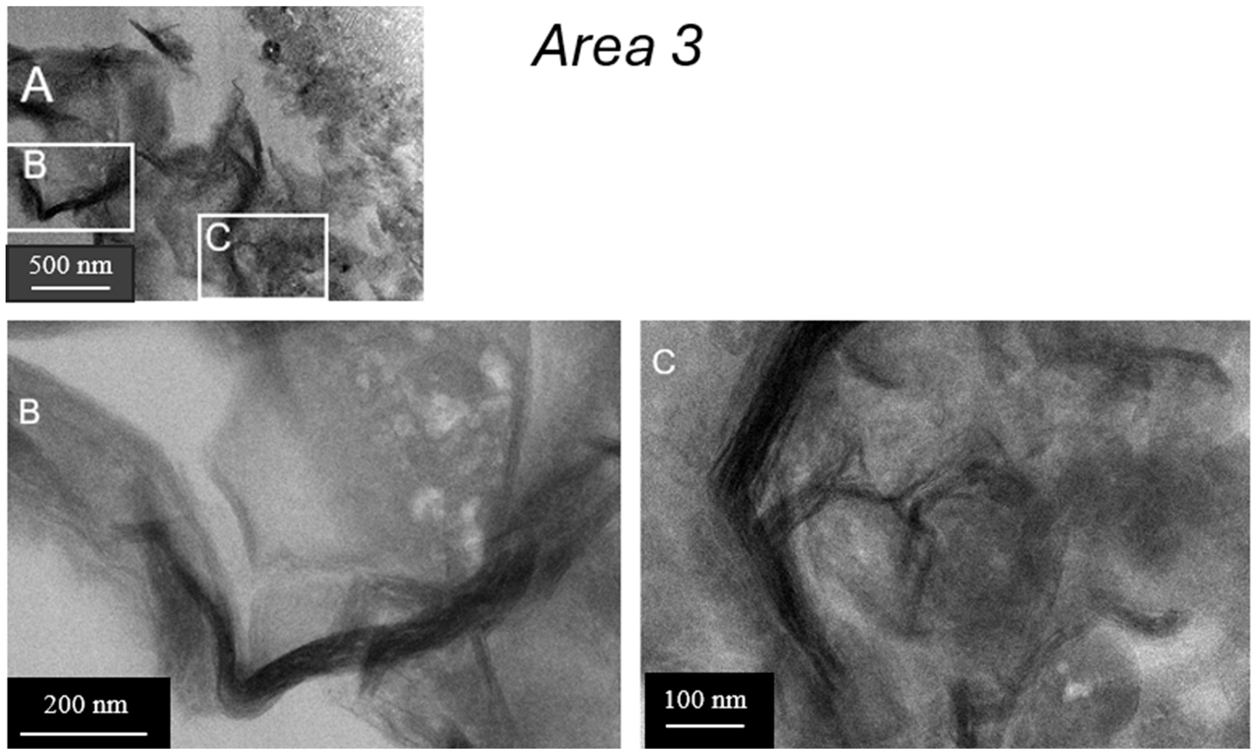
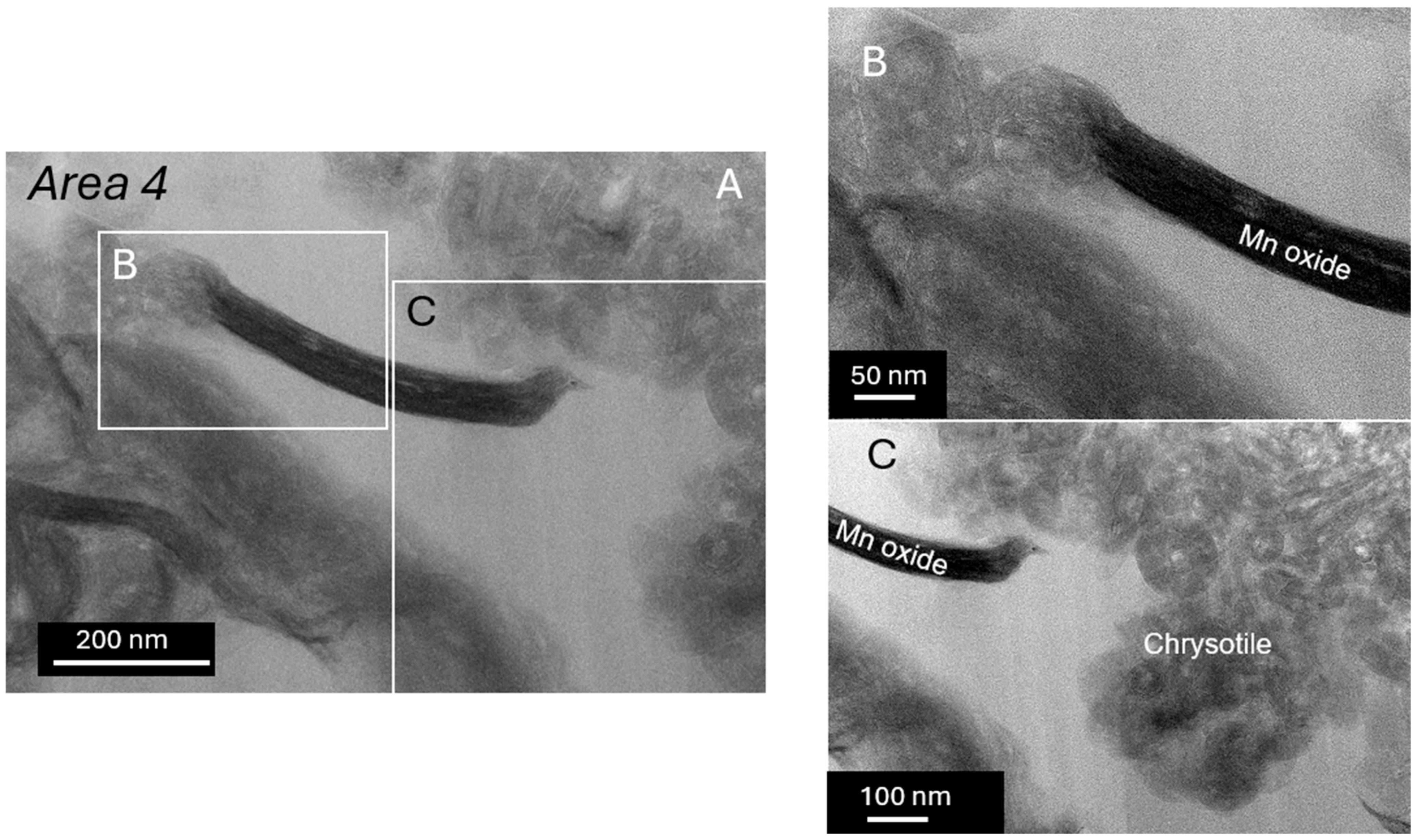
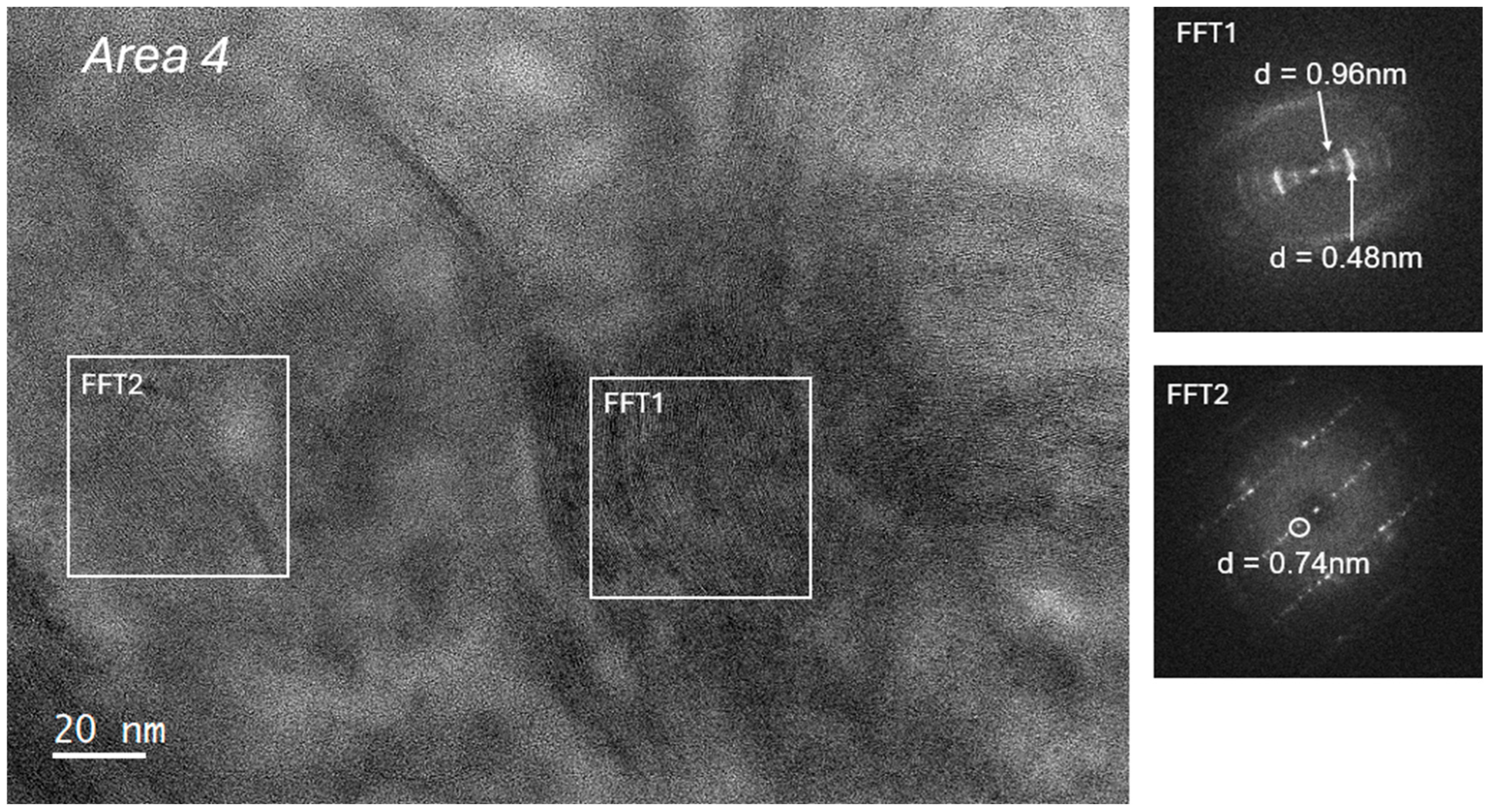
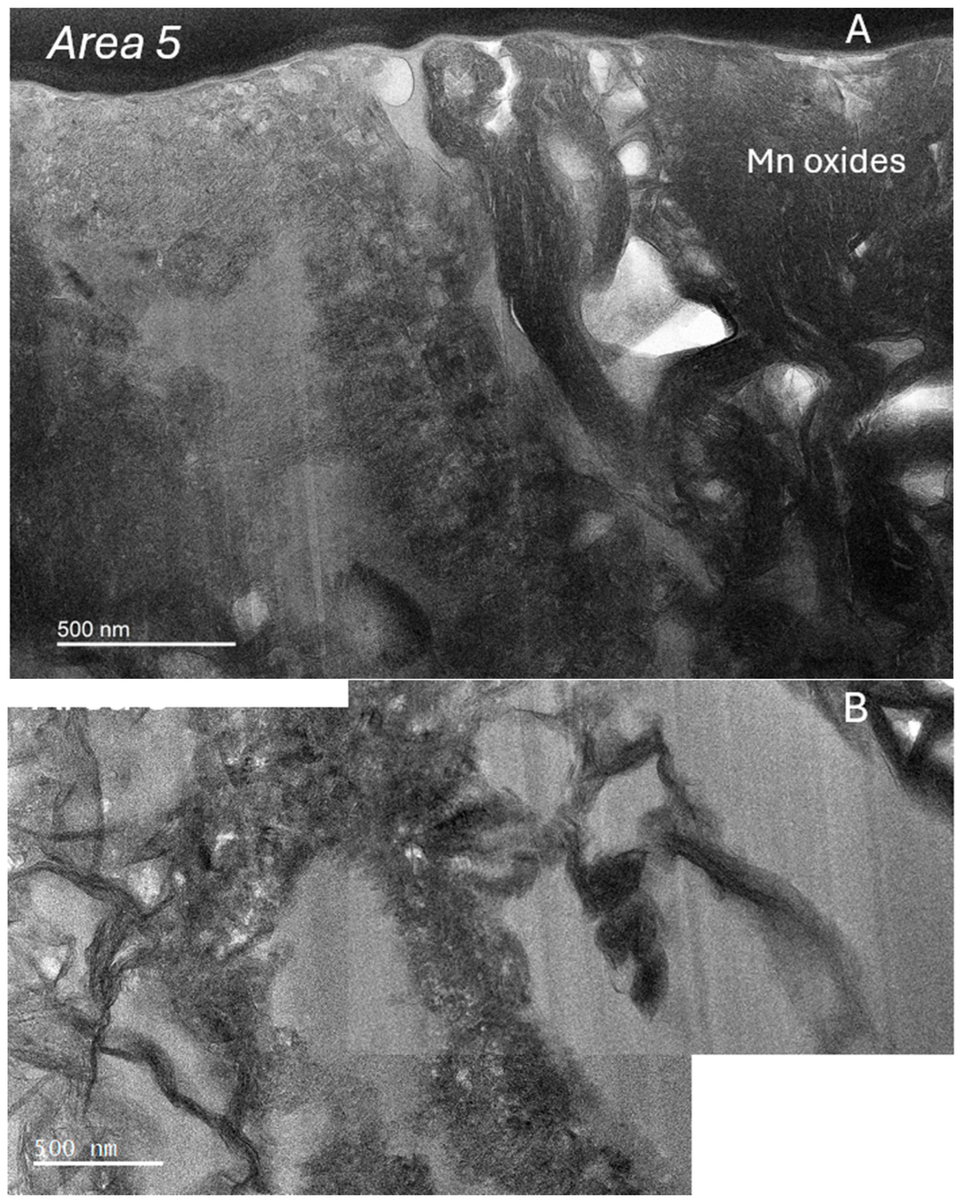
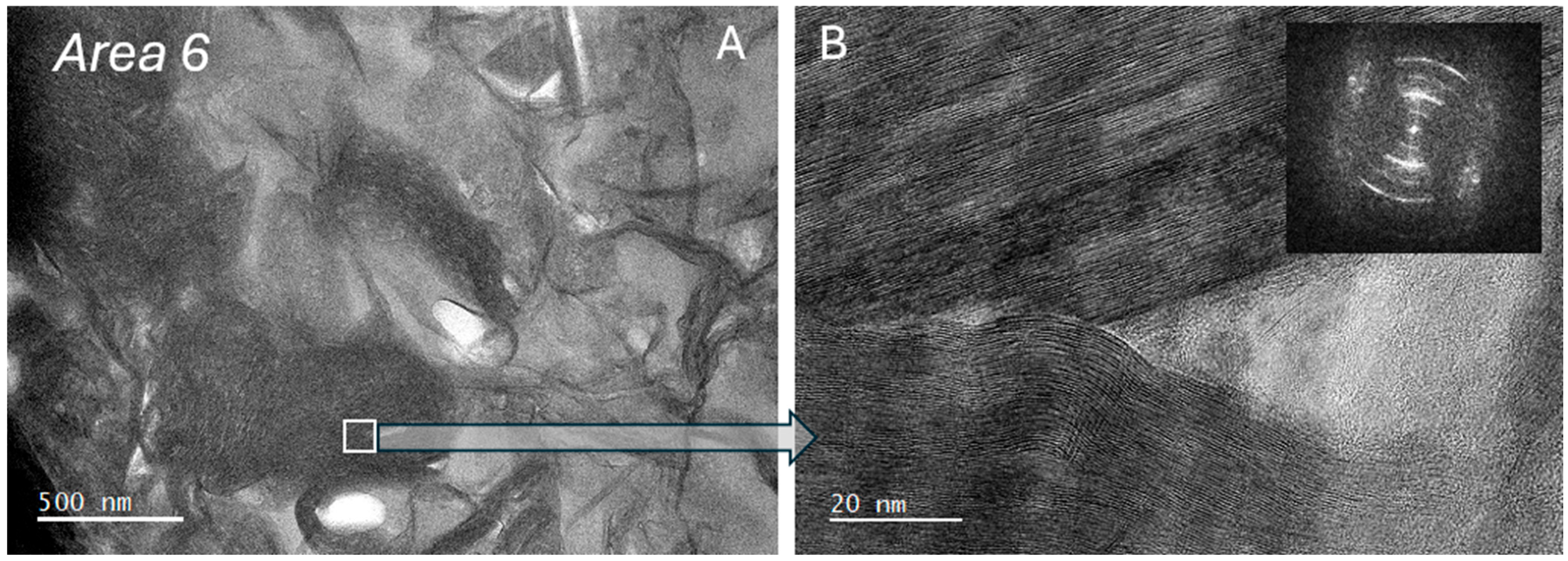
Typical chrysotile cross sections are seen in areas 2 (Figure 20) and 3 (Figure 21D). Areas 3, 4, 5, and 6 have good examples of Mn oxides (Figure 21B,C; Figure 22; Figure 23; Figure 24; Figure 25; Figure 26). The FFT pattern for vernadite, a monoclinic Mn oxide ((Mn⁴⁺, Fe³⁺, Ca, Na)(O, OH)₂ · nH₂O), is shown in Figure 24 FFT2 and in the FFT inset in Figure 26B. The monoclinic mineral todorokite ((Na, Ca, K, Ba, Sr)_1-x(Mn, Mg, Al)₆O₁₂ · 3-4H₂O) is a possible match for the FFT patterns and d spacing, but, as noted in the caption to Figure 24, the form of the mineral seems to point towards vernadite. This Mn hydrous oxide mineral, characterized by turbostratically stacked Mn-O layers, is thought to form biogenically by Mn-oxidizing bacteria [44].

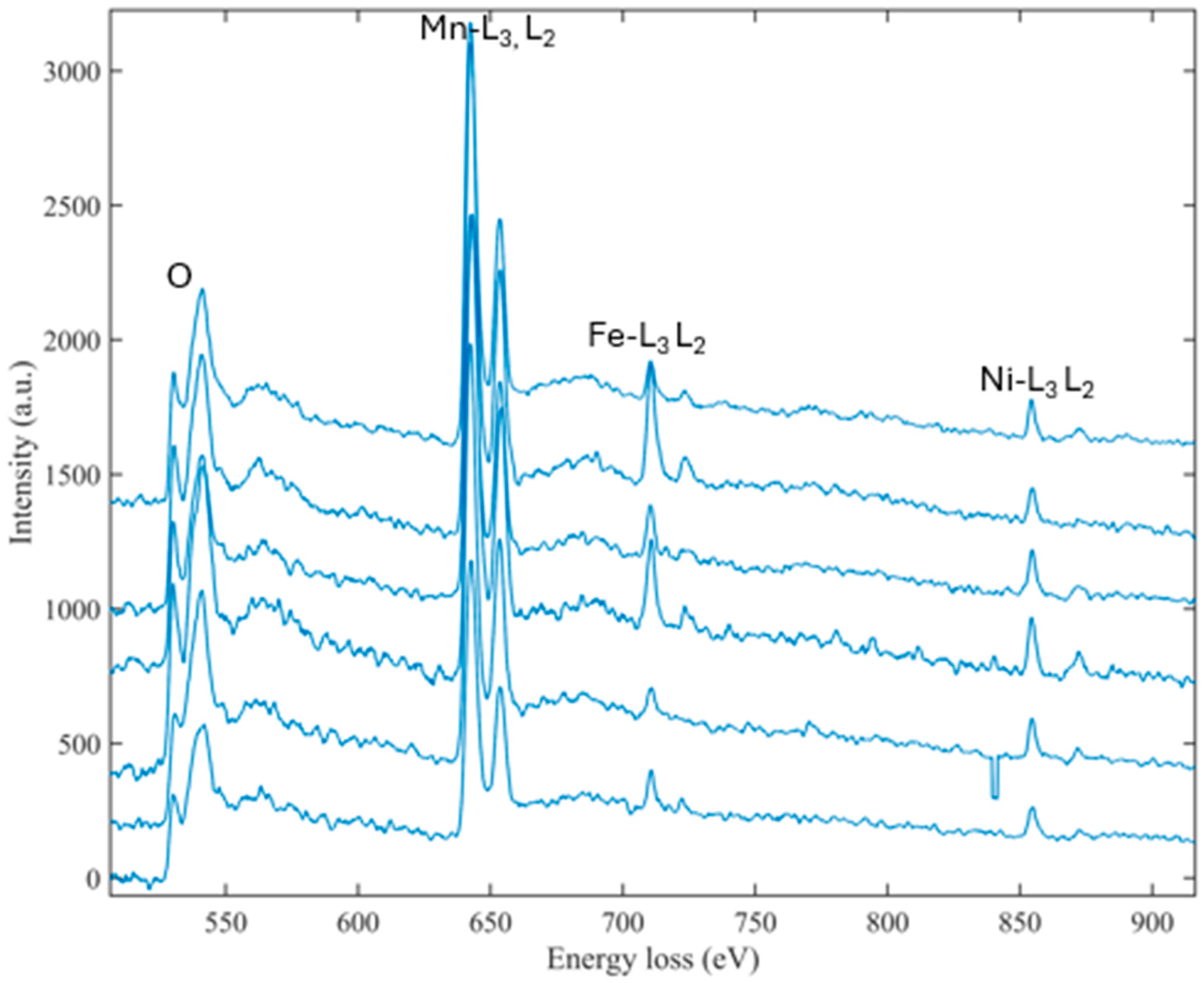
Several EELS spectra of Mn oxides were acquired in STEM mode by point analysis from areas 3 (Figure 21), 4 (Figure 23), and 6 (Figure 26). The high-loss region of the spectra (480–1050 eV) indicates that the Mn oxides host Fe and Ni, with Ni > Fe on average. Variations in Fe and Ni concentrations are evident in the background-subtracted, plural scattering-corrected EELS spectra (Figure 27; details are in Supplemental Files S6 and S7), but no systematic trends are observed either among different regions or within individual particles.

The fine structure of the Mn, Fe, and O edges in the EELS spectra varies as a function of oxidation state [38,45]. Based on the Mn L3/L2 white-line intensity ratio [38], the Mn oxides are characterized by a mixed Mn⁴⁺/Mn³⁺ oxidation state, with locally variable proportions but consistently higher Mn⁴⁺ than Mn³⁺. The ELNES of oxygen (Figure 27), characterized by a pre-edge peak, further supports the prevalence of Mn⁴⁺ [45]. Variations in the relative intensity of the pre-edge peak with respect to the main edge indicate local variability in the oxidation state. The EELS spectra also suggest variability in the Fe oxidation state within the Mn oxides, whereas acquisitions from discrete iron oxides indicate Fe³⁺. Vernadite is known to host Ni in other settings [46] and is a highly reactive Mn oxide that effectively sorbs metals during weathering due to its poor crystallinity [44]. The local oxidation state variations identified by EELS contribute to the disordered structure of this mineral and enhance its reactivity.

Figure 24. Transmission electron micrograph of area 4. Lizardite or chrysotile (FFT2; d-space = 0.74) in the Mn-oxides region. The Mn-oxide spots with d-space of 0.96 and 0.48 match either todorokite or vernadite (FFT1). Todorokite, however, forms rigid needles that grow at 120° angles. Vernadite is known to have a layered structure with turbostratic disorder, more similar to what these images show [47]. Scale = 20 nm.

Figure 24. Transmission electron micrograph of area 4. Lizardite or chrysotile (FFT2; d-space = 0.74) in the Mn-oxides region. The Mn-oxide spots with d-space of 0.96 and 0.48 match either todorokite or vernadite (FFT1). Todorokite, however, forms rigid needles that grow at 120° angles. Vernadite is known to have a layered structure with turbostratic disorder, more similar to what these images show [47]. Scale = 20 nm.

Figure 25. Transmission electron micrographs of area 5 (A,B) Mn oxides. Scale = 500 nm.

Figure 25. Transmission electron micrographs of area 5 (A,B) Mn oxides. Scale = 500 nm.

Figure 26. Transmission electron micrographs of area 6. (A) Mn oxides with location of inset (B). Scale = 500 nm. (B) Mn oxides at the surface after additional thinning. The d-spacing of lattice fringes, measured from the innermost ring of the corresponding FFT (upper right corner), is 0.96 nm, consistent with todorokite or vernadite. Several EELS spectra were collected from this region. Scale = 20 nm.

Figure 26. Transmission electron micrographs of area 6. (A) Mn oxides with location of inset (B). Scale = 500 nm. (B) Mn oxides at the surface after additional thinning. The d-spacing of lattice fringes, measured from the innermost ring of the corresponding FFT (upper right corner), is 0.96 nm, consistent with todorokite or vernadite. Several EELS spectra were collected from this region. Scale = 20 nm.

Figure 27. Stack of representative EELS spectra, after background subtraction and correction for plural scattering. Manganese and Fe oxidation states were estimated using the L₃/L₂ white-line intensity ratios. The oxygen ELNES features further reflect variations in Mn oxidation state.

Figure 27. Stack of representative EELS spectra, after background subtraction and correction for plural scattering. Manganese and Fe oxidation states were estimated using the L₃/L₂ white-line intensity ratios. The oxygen ELNES features further reflect variations in Mn oxidation state.

3.4. Discussion

Minerals determined via SEM and TEM are listed in

Table 2. Minerals identified via XRD ref. [33] and electron microscopy.

XRD	lizardite +/− antigorite; dolomite; clinochlore (?); chromite (?); quartz; talc
SEM	magnetite; “chromite” (albeit, not the ideal chromite composition); gahnite; clinochlore; antigorite; Si > Mg > Mn >> Fe ≈ Ni > Al mineral in the lizardite subgroup
TEM	chrysotile; vernadite; todorokite (?)

[Note that the TEM area was spatially restricted. Only minerals solely identified via TEM are listed here.].

. Most of the observed minerals serve to confirm the XRD identifications; the value of the SEM and TEM examination is in the identification of minerals not present at the levels necessary for XRD identification and for the delineation of the chemistry of these minerals. As determined in the original study [33], the study samples have high MgO, Ni, Cr, and Mn concentrations with lizardite (Triclinic; Mg₃Si₂O₅(OH)₄), antigorite (Monoclinic; (Mg, Fe)₃Si₂O₅(OH)₄), and chrysotile (Monoclinic; Mg₃Si₂O₅(OH)₄) being the most abundant minerals. Lizardite is an end member of the Lizardite-Népouite (Ni₃Si₂O₅(OH)₄) series, so some degree of substitution of Ni for Mg is expected. Other Mg-bearing minerals include clinochlore (Mg, Fe⁺⁺)₅Al(Si₃Al)O₁₀(OH)₈), dolomite (CaMg(CO₃)₂), talc (Mg₃Si₄O₁₀(OH)₂), diopside (MgCaSi₂O₆), and biotite (K(Mg,Fe)₃AlSi₃O₁₀(F,OH)₂). Chromite (Fe⁺⁺Cr₂O₄), the Cr-rich spinel, and the foundation of the world-class chrome industry in the 1800s, is also a common mineral.

The SEM-EDS investigations demonstrated that the “chromite” does not meet the expected 2:1 Cr:Fe ratio, although the discrepancy could be due to the EDS measuring a volume with a mix of chromite, magnetite, and possibly other spinel minerals. At this scale, it is not possible to determine if this analysis is typical of the chromite once mined throughout the State Line Serpentinite Belt. Overall, the region was, for its time in the mid-1800s, a world-class source of chromite; thus, a deviation from an ideal chromite chemistry was not a problem. An EDS scan of a magnetite grain showed trace amounts of Mg, Al, Mn, and Ni. As with the chromite noted above, these elements could be present in the spinel structure and/or in other minerals within the area measured by EDS.

Other minerals scanned by EDS included Mg-rich clinochlore with no detectable Fe, Si > Mg > Mn >> Fe ≈ Ni > Al lizardite, Mg ≈ Si lizardite, and gahnite (ZnAl₂O₄), an Al-group spinel mineral.

But what about the abundant Mn noted in the chemical analyses (after [33]; Supplemental File S1 Table S1)? The region selected for FIB liftout and further TEM-EDS examination has abundant Mn oxides, chrysotile, antigorite, and amorphous phases. Cross sections of chrysotile are seen as rounded fibers. Antigorite, having a structure with periodic contrast reversal of the SiO₂ tetrahedra with a modulation of ~3.3 nm, is surrounded by an amorphous phase containing sparse chrysotile fibers. Based on the FFT pattern, the Mn oxide is vernadite, a monoclinic Mn oxide ((Mn⁴⁺, Fe³⁺, Ca, Na)(O, OH)₂ · nH₂O). EELS spectra of Mn oxides were acquired from several points in three areas of the FIB specimen. The Mn oxides host Fe and Ni, with a general trend of Ni > Fe. The Mn L3/L2 white-line intensity ratio [38] demonstrates that the Mn oxides are characterized by a mixed Mn⁴⁺/Mn³⁺ oxidation state, with Mn⁴⁺ consistently greater than Mn³⁺. Within the vernadite, Ni is generally more abundant than Fe. The oxidation state of Fe within the Mn oxides is variable, in contrast to the Fe³⁺ found in discrete Fe oxides.

4. Conclusions

The State Line Serpentinite Belt in Chester and Lancaster counties, Pennsylvania, and Cecil County, Maryland, was an important source of chromite, asbestos, and magnesia in the mid-1800s. Hower et al. [33], in a study focusing on maceral development, discussed the MgO-, Mn-, Cr-, and Ni-rich soils developed at Goat Hill, Chester County, Pennsylvania. Their samples provided the basis for this scanning and transmission electron microscopic study of the samples.

The mineral suites identified by XRD are dominated by lizardite, antigorite, chrysotile, clinochlore, dolomite, talc, diopside, biotite, Mn oxides, and chromite. The SEM-EDS examination showed that the chromite did not meet the expected 2:1 Cr:Fe ratio, perhaps due to other spinel minerals falling within the volume analyzed by EDS. Similarly, magnetite showed trace amounts of Mg, Al, Mn, and Ni, all possible within the spinel structure but potentially occurring within minerals other than magnetite. Gahnite (ZnAl₂O₄), an Al-group spinel mineral, was found. Mg-rich clinochlore and lizardite, with little or no Fe, dominated the mineral assemblages.

The TEM-EDS, along with EELS studies, demonstrated the presence of vernadite as the Mn oxide form. The Mn oxides contain Fe and Ni, generally with Ni > Fe. The EELS Mn L3/L2 white-line intensity ratio [38] demonstrates that the Mn oxides have a mixed Mn⁴⁺/Mn³⁺ oxidation state, with Mn⁴⁺ > Mn³⁺. Nickel is more abundant than Fe, and the Fe oxidation state within the vernadite is variable.

Overall, all studies are defined by their scale. A scanning and transmission electron microscopic study can reveal chemical and crystalline details that are not discernible in petrographic and XRD mineralogy studies. While the breadth of the sample set and the number of TEM specimens per sample may be limited by time and budget, such limitations should not discourage further exploration of this deposit or similar rocks. Any investigation at any scale has the potential to reveal details that help to refine the nature of the deposit.

References

1. Crowley, W.P. Tectonic emplacement of the Baltimore gabbro complex. Geol. Soc. Am. Abstr. Programs 1973, 5, 10. [Google Scholar]
2. Crowley, W.P. Post-Grenville, pre-metamorphic history of the eastern Maryland Piedmont. Geol. Soc. Am. Abstr. Programs 1975, 7, 43. [Google Scholar]
3. Morgan, B.A. The Baltimore Complex, Maryland, Pennsylvania and Virginia. In Oregon Department of Geology and Mineral Industries Bulletin; Coleman, R., Ed.; North American Ophiolites; State of Oregon, Department of Geology and Mineral Industries: Portland, OR, USA, 1977; Volume 95, pp. 41–49. [Google Scholar]
4. Crawford, M.L.; Crawford, W.A.; Hoersch, A.L.; Wagner, M.E. Precambrian and Lower Paleozoic—Selected metamorphic and igneous rocks rocks of the Piedmont upland. In The Geology of Pennsylvania, Pennsylvania Geological Survey Special Publication; Schultz, C.H., Ed.; Pennsylvania Department of General: Harrisburg, PA, USA, 1999; Volume 1, pp. 27–35. [Google Scholar]
5. Bascom, F. The geology of the crystalline rocks of Cecil County, Maryland. In Cecil County, Maryland Geological Survey; Forgotten Books: London, UK, 1902; Volume 1, pp. 83–148. [Google Scholar]
6. Higgins, M.W. Depth of emplacement of James Run Formation pillow basalts, and the depth of deposition of part of the Wissahickon Formation, Appalachian Piedmont, Maryland. Am. J. Sci. 1971, 271, 321–332. [Google Scholar] [CrossRef]
7. Higgins, M.W. Age, Origin, Regional Relations, and Nomenclature of the Glenarm Series, Central Appalachian Piedmont: A Reinterpretation. Geol. Soc. Am. Bull. 1972, 83, 989–1026. [Google Scholar] [CrossRef]
8. Faill, R.T. A geologic history of the North-central Appalachians. Part 1. Orogenesis from the Mesoproterozoic through the Taconic orogeny. Am. J. Sci. 1997, 297, 551–619. [Google Scholar] [CrossRef]
9. Gordon, S.G. Ordovician basalts and quartz diabases in Lebanon County, Pennsylvania. Acad. Nat. Sci. Phila. Proc. 1921, 72, 354–357. [Google Scholar]
10. Stose, G.W.; Jonas, A.I. Ordovician shale and associated lava in southeastern Pennsylvania. Geol. Soc. Am. Bull. 1927, 38, 505–536. [Google Scholar] [CrossRef]
11. Lash, G.G. Sedimentologic and geochemical evidence for Ordovician near-trench volcanism in the Central Appalachian orogeny. J. Geol. 1986, 94, 91–107. [Google Scholar] [CrossRef]
12. Ashcroft, T.J. Field Relations, Structural Geology, and Geochemistry of the Jonestown Volcanic Field, Lebanon County, Southeastern Pennsylvania. Master’s Thesis, State University of New York, Albany, NY, USA, 2002; 111p. [Google Scholar]
13. Ganis, G.R.; Wise, D.U. Taconic events in Pennsylvania: Datable phases of a ∼20 M.Y. orogeny. Am. J. Sci. 2008, 308, 167–183. [Google Scholar] [CrossRef]
14. Wise, D.U.; Ganis, G.R. Taconic orogeny in Pennsylvania: A ~15–20 m.y. Apennine-style Ordovician event viewed from its Martic hinterland. J. Struct. Geol. 2009, 31, 887–899. [Google Scholar] [CrossRef]
15. Schoonmaker, A.; Kidd, W.S.F.; Ashcroft, T. Magmatism and extension in the foreland and near-trench region of collisional and convergent tectonic systems. Geosci. Can. 2016, 43, 159–178. [Google Scholar] [CrossRef][Green Version]
16. Southwick, D.L. Structure and petrology of the Harford County part of the Baltimore—State Line gabbro—Peridotite complex. In Studies of Appalachian Geology: Central and Southern; Fisher, G.W., Pettijohn, P.J., Reed, J.C., Weaver, K., Eds.; Wiley Interscience: New York, NY, USA, 1970; pp. 397–415. [Google Scholar]
17. Crowley, W.P. The geology of the crystalline rocks near Baltimore and its bearing on the evolution of the eastern Maryland Piedmont. In Maryland Geological Survey Report of Investigations; Maryland Geological Survey: Baltimore, MA, USA, 1976; Volume 27, 39p. [Google Scholar]
18. Sinha, A.K.; Hanan, B.B.; Sans, J.R.; Hall, S.T. Igneous rocks of the Maryland Piedmont: Indicators of crustal evolution. In The Caledonides in the USA. International Geologic Correlation Program Project 27; Wones, D.R., Ed.; Polytechnic Institute & State University: Blacksburg, VA, USA, 1980; pp. 131–135. [Google Scholar]
19. Shaw, H.F.; Wasserburg, G.J. Isotopic constraints on the origin of Appalachian mafic complexes. Am. J. Sci. 1984, 284, 319–349. [Google Scholar] [CrossRef]
20. Freedman, J.; Wise, D.U.; Bentley, R.D. Pattern of folded folds in the Appalachian Piedmont along Susquehanna River. Geol. Soc. Am. Bull. 1964, 75, 621–638. [Google Scholar] [CrossRef]
21. Lapham, D.M.; McKague, H.L. Structural patterns associated with the serpentinites of southeastern Pennsylvania. Geol. Soc. Am. Bull. 1964, 75, 639–660. [Google Scholar] [CrossRef]
22. Wise, D.U. Multiple deformation, geosynclinal transitions, and the Martic problem in Pennsylvania. In Studies of Appalachian Geology: Central and Southern; Fisher, G.W., Pettijohn, P.J., Reed, J.C., Weaver, K., Eds.; Wiley Interscience: New York, NY, USA, 1970; pp. 317–333. [Google Scholar]
23. Muller, P.D.; Chapin, D.A. Tectonic evolution of the Baltimore Gneiss anticlines, Maryland. In The Grenville Event in the Appalachians and Related Topics, Geological Society of America Special Paper; Bartholomew, M.J., Ed.; The Geological Society of America: Boulder, CO, USA, 1984; Volume 194, pp. 127–148. [Google Scholar]
24. Wagner, M.E.; Srogi, L. Early Paleozoic metamorphism at two crustal levels and a tectonic model for the Pennsylvania-Delaware Piedmont. Geol. Soc. Am. Bull. 1987, 99, 113–126. [Google Scholar] [CrossRef]
25. Dmochowski, J. Geology of Philadelphia and NW suburbs. In National Association of Geoscience Teachers; Eastern Section Field Trip: Mumbai, MA, USA, 2010; Volume 27, p. + appended reprints. [Google Scholar]
26. Gordon, S.G. The chromite deposits of the State Line serpentines. Acad. Nat. Sci. Phila. Proc. 1921, 73, 449–454. [Google Scholar]
27. Lapham, D.M. Preliminary Report on the Chromite Occurrence at the Wood Mine, Pennsylvania; Pennsylvania Geological Survey, 4th series, Progress Report; Bureau of Topographic & Geological Survey: Middletown, PA, USA, 1958; Volume 153, 11p.
28. Ulmer, G.C. Alteration of chromite during serpentinization in the Pennsylvania-Maryland District. Am. Mineral. 1974, 59, 1236–1241. [Google Scholar]
29. Knopf, E.B. Chrome ores of southeastern Pennsylvania and Maryland. In U.S. Geological Survey Bulletin; U.S. Government Publishing Office: Washington, DC, USA, 1921; Volume 725, pp. 85–99. [Google Scholar]
30. Pearre, N.C.; Heyl, A.V., Jr. Chromite and Other Mineral Deposits in Serpentine Rocks of the Piedmont Upland, Maryland, Pennsylvania and Delaware, 1082-K. U.S. Geological Survey Bulletin; U.S. Government Publishing Office: Washington, DC, USA, 1960.
31. Gates, A.E. Shear zone control on mineral deposits in the State-line serpentinite, Pennsylvania Piedmont. Ore Geol. Rev. 1991, 6, 171–184. [Google Scholar] [CrossRef]
32. Wylie, A.G.; Candela, P.A. Metallic mineral deposits—Chromite. In The Geology of Pennsylvania. Pennsylvania Geological Survey Special Publication; Schultz, C.H., Ed.; Pennsylvania Department of General: Harrisburg, PA, USA, 1999; Volume 1, pp. 589–595. [Google Scholar]
33. Hower, J.C.; O’Keefe, J.M.K.; Latham, R.E.; Dai, S.; Silva, L.F.O.; Henke, K.R.; Thorson, J.S. Organic petrology, palynology, and geochemistry of soils from serpentine barrens, Chester and Lancaster counties, Pennsylvania: Notes on maceral development. Int. J. Coal Geol. 2024, 289, 104532. [Google Scholar] [CrossRef]
34. Rajakaruna, N.; Harris, T.B.; Alexander, E.B. Serpentine geoecology of eastern North America: A review. Rhodora 2009, 111, 21–108. [Google Scholar] [CrossRef]
35. Brooks, R.R. Serpentine and Its Vegetation: A Multi-Disciplinary Approach; Dioscorides Press: Portland, OR, USA, 1987; 454p. [Google Scholar]
36. Scott, J.; Thomas, P.J.; MacKenzie, M.; McFadzean, S.; Wilbrink, J.; Craven, A.J.; Nicholson, W.A.P. Near-simultaneous dual energy range EELS spectrum imaging. Ultramicroscopy 2008, 108, 1586. [Google Scholar] [CrossRef]
37. Malis, T.; Cheng, S.C.; Egerton, R.F. EELS log ratio technique for specimen-thickness measurement in the TEM. J. Electron Microsc. Tech. 1988, 8, 193. [Google Scholar] [CrossRef]
38. Van Aken, P.A.; Liebscher, B.; Styrsa, V.J. Quantitative determination of iron oxidation states in minerals using Fe L 2, 3-edge electron energy-loss near-edge structure spectroscopy. Phys. Chem. Miner. 1998, 25, 323–327. [Google Scholar] [CrossRef]
39. Stroud, R.M.; Singerling, S.A. Fundamentals of transmission electron microscopy in earth and planetary sciences. In Treatise on Geochemistry, 3rd ed.; Elsevier: Amsterdam, The Netherlands, 2025; Volume 8, pp. 861–881. [Google Scholar]
40. Palache, C.; Berman, H.; Frondel, C. The System of Mineralogy of James Dwight Dana and Henry Salisbury Dana: Yale University 1837–1892: Volume I: Elements, Sulfides, Sulfosalts, Oxides, 7th ed.; Wiley: New York, NY, USA, 1944; 834p. [Google Scholar]
41. Picot, P.; Johan, Z. Atlas des mineraux metalliques. In Mémoires du Bureau de Recherches Géologiques et Minières; BRGM: Orléans, France, 1977; Volume 90-1977, 403p. [Google Scholar]
42. Ramdohr, P. The Ore Minerals and Their Intergrowths, 2nd ed.; English Translation of the Fourth Edition, with Additions and Corrections by the Author; Pergamon Press: Oxford, UK, 1980; 1205p. [Google Scholar]
43. Dódony, I.; Pósfai, M.; Buseck, P.R. Revised structure models for antigorite: An HRTEM study. Am. Mineral. 2002, 87, 1443–1457. [Google Scholar] [CrossRef]
44. Hochella, M.F., Jr.; Kasama, T.; Putnis, A.; Putnis, C.V.; Moore, J.N. Environmentally important, poorly crystalline Fe/Mn hydrous oxides: Ferrihydrite and a possibly new vernadite-like mineral from the Clark Fork River Superfund Complex. Am. Mineral. 2005, 90, 718–724. [Google Scholar] [CrossRef]
45. Tan, H.; Verbeeck, J.; Abakumov, A.; Van Tendeloo, G. Oxidation state and chemical shift investigation in transition metal oxides by EELS. Ultramicroscopy 2012, 116, 24–33. [Google Scholar] [CrossRef]
46. Bodeï, S.; Manceau, A.; Geoffroy, N.; Baronnet, A.; Buatier, M. Formation of todorokite from vernadite in Ni-rich hemipelagic sediments. Geochim. Cosmochim. Acta 2007, 71, 5698–5716. [Google Scholar] [CrossRef]
47. Lee, S.; Xu, H.; Xu, W.; Sun, X. The structure and crystal chemistry of vernadite in ferromanganese crusts. Struct. Sci. 2019, 75, 591–598. [Google Scholar] [CrossRef]
Figure 1. Location of the Goat Hill Barrens in southwestern Chester County, Pennsylvania. The Nottingham County Park and New Texas sites were studied by Hower et al. [33]. The inset map of the State Line Serpentinite Belt study area is from Google Earth with the base map after Brooks [35]. The black areas in the regional map are locations of serpentinite occurrences. The Pennsylvania/Maryland state line is at 39°43′15″ N. The 76°00′ W and 76°15′ W meridians and the 39°41′ N parallels are marked on the inset map. Figure after Hower et al. [33].
Minerals 16 00302 g001
Figure 2. Scanning electron microscopy images of Fe-bearing spinels, with and without Cr. (A) Fe-Cr spinels; sample 2, area 1, spots 1 and 3; (B) yellow arrows: Fe-Cr spinels; sample 2, supplemental run, area 2, spots 1 and 2. Green arrow: magnetite; sample 2, supplemental run, area 3, spot 1; (C) magnetite; sample 2, supplemental run, area 4, spot 1; (D) magnetite; sample 2, supplemental run, area 6, spot 1; (E) magnetite; sample 2, supplemental run, area 7, spot 2. Spinel classifications after http://webmineral.com/data/Spinel.shtml (accessed on 16 February 2026).
Minerals 16 00302 g002
Figure 3. SEM-EDS spectra from 5.0 to 8.0 keV. (A) Full-count (>2000 counts) EDS spectra, including all spinels shown in Figure 2. (B) EDS spectra for the Fe-Cr spinels are shown in Figure 2A,B. Note that the Fe Kα peak is truncated at 1000 counts in order to provide better resolution of the Cr Kα and Cr Kβ peaks. The Area2_EDS SA 2 supp. peaks are emphasized since it has the largest Cr Kα and the smallest Fe Kα peaks among the points analyzed. All EDS data are in the Supplemental Files S2–S5.
Minerals 16 00302 g003
Figure 4. Scanning electron micrographs of Goat Hill site 2, areas 5 (A) and 7 (B). The EDS spectra for selected areas 1 on both (A,B) are shown in Figure 5.
Minerals 16 00302 g004
Figure 5. Goat Hill site 2, areas 5 and 7 SEM-EDS spectra from 0.55 to 2.0 keV (A) and 5.5 to 8.0 keV (B). The significant Fe peaks indicate that the minerals are Fe-spinels (magnetite). Minor Mn, Ni, Mg, Si, and Al peaks are present. All EDS data are in the Supplemental Files S2–S5.
Minerals 16 00302 g005
Figure 6. Scanning electron micrograph of Goat Hill site 1, area 2.
Minerals 16 00302 g006
Figure 7. Goat Hill site 1, area 10, selected area 2 EDS spectra from 0 to 4 keV. The Al Kα peak is truncated at 200 counts in order to emphasize the Mg and Ca Kα peaks. All EDS data are in the Supplemental Files S2–S5.
Minerals 16 00302 g007
Figure 8. Scanning electron micrograph of Goat Hill site 1, area 1, spot 1. All EDS data are in the Supplemental Files S2–S5.
Minerals 16 00302 g008
Figure 9. Goat Hill site 1, area 1, spot 1 spectra from 0.0 to 2.5 keV (A) emphasizing the rod-like crystal (spot 1) and another mineral (spot 5) with more Mn, Fe, and Ni than the spot 1 mineral. The energy range from 5.0 to 8.0 keV (B) shows the previous two spots plus spots 3 and 4. All EDS data is in the Supplemental Files S2–S5.
Minerals 16 00302 g009
Figure 10. Scanning electron micrographs of Goat Hill site 1, area 11, selected area 1. All EDS data is in the Supplemental Files S2–S5.
Minerals 16 00302 g010
Figure 11. Goat Hill area 11, selected area 1, EDS spectra from 0 to 2.5 keV (A) and from 8.33 to 10 keV (B). All EDS data are in the Supplemental Files S2–S5.
Minerals 16 00302 g011
Figure 12. Scanning electron micrograph of Goat Hill site 1, area 7. Spots 2 and 6 are highlighted in Figure 13. All EDS data is in the Supplemental Files S2–S5.
Minerals 16 00302 g012
Figure 13. Goat Hill site 1, area 7, EDS spots 2 and 6 spectra from 0 to 4 keV (A), 0.55 to 1.0 keV (B), and 5.5 to 8.0 keV (C). All EDS data are in the Supplemental Files S2–S5.
Minerals 16 00302 g013
Figure 14. Scanning electron micrograph of Goat Hill site 1, area 12, spots 1, 2, and 3.
Minerals 16 00302 g014
Figure 15. Goat Hill site 1, area 12, spots 1, 2, and 3 EDS spectra from 0 to 2.5 keV with an inset from 2.0 to 2.5 keV for 0 to 170 counts (compared to more than 8000 counts for the full spectrum) (A) and for 6.0 to 7.5 keV (B). All EDS data are in the Supplemental Files S2–S5.
Minerals 16 00302 g015
Figure 16. (A) BSE image shows a larger view of the pellet where the (B) FIB section was traced. B is a repeat of Figure 12, with the addition of the FIB trace. Figure 8 is an image of a portion of the same grain. The annotations of chrysotile, amorphous, and antigorite are based on the TEM of the FIB section. (C) Location of areas discussed in Figure 17, Figure 18, Figure 19, Figure 20, Figure 21, Figure 22, Figure 23, Figure 24, Figure 25 and Figure 26.
Minerals 16 00302 g016
Figure 17. Transmission electron micrograph. (A) Area 1 with antigorite and amorphous phases with chrysotile inclusions. The location of (B) is shown. (B) Selected area of (A). Scale = 100 nm. (C) FFT of antigorite with simulated diffraction. Scale = 20 nm.
Minerals 16 00302 g017
Figure 18. Transmission electron micrograph. Area 1. (A) HRTEM of antigorite. Scale = 10 nm. (B) FFT filtered image of the region marked by the white rectangle that shows the periodic contrast reversal. The Scale = 5 nm. (C) Antigorite structure projection of the 010 plane showing the modulated structure with the periodic inversion of the Si-oxide tetrahedra. (D) Projection on the 001 plane. Structure image generated using Vesta from the amcsd 0004123 entry. The antigorite in the experimental images differs from the model in that the inversion occurs after fewer SiO2 tetrahedra, giving a smaller cell a-axis.
Minerals 16 00302 g018
Figure 19. Transmission electron micrographs. Area 1. Amorphous region at the edge of the antigorite. Scale = 100 nm. FFT1: amorphous phase. FFT2: rings with radius d-space of r1 = 0.74 nm and r2 = 0.372 nm, consistent with the d(001) of serpentine minerals.
Minerals 16 00302 g019
Figure 20. Transmission electron micrographs. (A) Area 2 with locations of (B,C). Scale = 500 nm. (B) Chrysotile and chrysotile + amorphous phase mix. Scale = 100 nm. (C) Chrysotile. Scale = 100 nm.
Minerals 16 00302 g020
Figure 21. Transmission electron micrographs. Area 3. (A) Chrysotile at the edge of the amorphous region surrounding the antigorite. Mn-oxide filaments are near the chrysotile. Locations of insets (BD) are indicated in (A). Scale = 500 nm. (B) Chrysotile with Mn-oxide filaments. Scale = 100 nm. (C) Mn-oxide filaments. Scale = 200 nm. (D) Chrysotile with an inset of the FFT diffraction pattern for the mineral. Scale = 100 nm.
Minerals 16 00302 g021
Figure 22. Transmission electron micrographs. Area 3. (A) Base image showing locations of insets (B,C). Scale 500 nm. (B) Mn oxides. Scale = 200 nm. (C) Mn oxides. Scale = 100 nm.
Minerals 16 00302 g022
Figure 23. Transmission electron micrographs. Area 4. (A) Base image showing locations of insets (B,C). Scale 200 nm. (B) Mn oxides. Scale = 50 nm. (C) Mn oxide and chrysotile. Scale = 100 nm.
Minerals 16 00302 g023