Article

Technical and Economic Impact of Geometallurgical Variables in a Mining Project

by
Leone Freire da Silva
1,*,
Kelly Cristina Ferreira
2,
Leonardo Junior Fernandes Campos
1 and
Douglas Batista Mazzinghy
1,*
1
Curso de Pós-Graduação em Engenharia Metalúrgica, Materiais e de Minas-Mestrado Profissional (CPGEM), Universidade Federal de Minas Gerais (UFMG), Belo Horizonte 31270-901, MG, Brazil
2
Departamento de Educação e Tecnologia-Núcleo de Metalurgia, Instituto Federal de Educação, Ciência e Tecnologia Sudeste de Minas Gerais-Campus Juiz de Fora, Juiz de Fora 36080-001, MG, Brazil
*
Authors to whom correspondence should be addressed.
Minerals 2026, 16(1), 40; https://doi.org/10.3390/min16010040 (registering DOI)
Submission received: 2 December 2025 / Revised: 22 December 2025 / Accepted: 24 December 2025 / Published: 29 December 2025
(This article belongs to the Special Issue Geometallurgy Applied to Mine Planning)

Abstract

The inherent complexity of the decision-making process in early-stage mining projects demands high-risk investments, often based on limited and low-confidence data. The geometallurgical approach offers an opportunity to mitigate uncertainties through the development of mathematical models to predict key process variables, such as recovery and specific energy. This research quantifies the economic and technical impact of incrementally increasing the number of variables in a geometallurgical model of a copper-gold-silver polymetallic deposit during the Pre-Feasibility Study (PFS) phase. Regression models were developed to correlate grades (copper, gold, and silver) and metallurgical variables (recovery and specific energy). The models were applied to eight geometallurgical block models, and technical and economic results were generated using Direct Block Sequencing (DBS). Across all scenarios, increased model complexity had a modest effect on production metrics but caused notable variation in Net Present Value (NPV), reaching a 6.92% difference between scenarios. Thus, adding more geometallurgical variables is justified not by higher production tonnage but by the potential to enhance and stabilize NPV through improved sequencing based on key value drivers (costs, recoveries and processing time). These findings highlight the value of early geometallurgical modeling, even with limited data, for producing a more integrated and improved economic assessment.

1. Introduction

Mining and mineral production are vital for the development of civilization, driven by population growth, industrial progress, technological development, and demands for renewable energy [1]. The increasing demand challenges industry, as lower-quality deposits require more resources for extraction [2]. One approach to improve efficiency is to incorporate geometallurgical modeling.
Geometallurgy is an integrated approach applied across the entire project life cycle, from studies in the early stages (Pre-Feasibility and Feasibility) to existing operations. It promotes sustainable mining by shifting the focus from simple mineral grade to a comprehensive understanding of the variable metallurgical response of the orebody, allowing improvements in mine planning, resource utilization, and ultimately project value [3,4]. However, the successful execution of this approach heavily relies on continuous data acquisition and methodological standardization across all project phases, an aspect that remains inconsistent in the industry.
This type of modeling combines fundamental rock characteristics (mineralogy, grades) with process variables (recovery, comminution) that respond block-by-block to guide and enhance every element of a mining project, including mine planning and sequencing, economic evaluations (NPV), and operational choices [5]. Efficiency is proven not only by allowing the plant to avoid productive bottlenecks from its conception but also by the possibility of improvements in equipment selection, reducing overall project costs.
Since 2000, the development of geometallurgical programs has significantly expanded [6,7], utilizing various spatial and statistical techniques, including kriging [8], principal component analysis (PCA) [9], and regression modeling [10]. Successful examples in operating mines consistently demonstrate the value of populating resource block models with key process metrics, such as comminution indices, for accurate prediction of plant throughput capacity [11,12,13,14]. Furthermore, studies have shown that incorporating geometallurgical variables into the sequencing of mining blocks can improve financial outcomes and increase ore productivity [15,16,17,18], while predictive modeling of recoveries has been successfully validated across various commodities [19,20]. Despite this, even with over 20 years of popularity, geometallurgy programs are still under development, as markets for different commodities are still discovering their potential for technical results and economic enhancements when considering this approach.
A significant limitation in the current geometallurgy literature is related to the fact that most publications are linked to operational projects. The search for published studies correlating geometallurgy with deposits in the early project phase is difficult, mainly due to the scarcity of initial data, which often lacks sufficient test results, robust technological characterization, and accurate spatial positioning of sample information, which are fundamental for the development of a robust model from the beginning of a project. Even in situations with a good level of available information, the current preference in project development is still for the adoption of assumptions based on statistical metrics of the project’s test results (e.g., 75th percentile). It is known that investment conditions in projects are the key factor for the decision of which type of approach should be considered, but even in projects with a good level of investment, the conservative/traditional choice is still the most applied.
Considering these inherent uncertainties, this research aims to address this challenge by providing an alternative perspective for integrating geometallurgical principles within this early-stage and data-limited context. This research presents a case study of a copper-gold-silver deposit in Brazil, which had its Pre-Feasibility Study (PFS) phase developed with a minimal quantity of tests but with adequate quality of available information. The original study developed the deposit’s mine plan and economics relying solely on recovery curves and fixed process variables—while employing a distinct mine sequencing methodology.
Regression models to establish relationships between deposit data (grades) and metallurgical variables, specifically recoveries (copper, gold, and silver), abrasion index, and specific energy, were developed and applied to the block models. Calculations for revenues and fixed and variable costs are mapped in the geometallurgical block models for subsequent use in the sequencing of mining blocks through the Direct Block Schedule (DBS) technique. The main technical results analyzed are run-of-mine (ROM) production, total material movement (ROM + waste), block processing time, and equivalent gold production. The main economic result analyzed is the Net Present Value (NPV) of the deposit, obtained from mine sequencing by Direct Block Sequencing (DBS).
The goal of this study is to map the impacts that an increase in the number of variables in the geometallurgical block model has on the technical and economic results of the mine sequencing of the polymetallic deposit under study, which is in the initial project phase. The hypothesis to be tested is that integrating complex geometallurgical variables into a block model would return not only more realistic and potentially higher Net Present Value (NPV) by enabling value-driven block selection via Direct Block Sequencing, but also a small impact on technical production metrics, such as run-of-mine production.

2. Materials and Methods

2.1. Disclaimer

The data for this study were obtained from publicly available reference NI 43-101 reports [21,22]. This work focuses specifically on the application of geometallurgical principles to the deposit to address the stated research objectives. There is no intention to compare the results obtained in this paper with those from the reference study, since the methodologies applied for geometallurgical modeling, sample selection, and mine sequencing are entirely different. It was assumed that the underlying data and test results adhere to industry’s best practices consistent with the Pre-Feasibility Study (PFS) level.

2.2. Overall Study Methodology

The sequence of activities to develop this study is presented in Figure 1. More details on study methodology are presented in the following sections.

2.3. Testwork Results Database

A total of 29 drill core samples were submitted for testwork. The samples were selected to ensure representativeness across the orebody in terms of both geological variability and spatial coverage. Figure 2 presents the distribution of the drillholes from which these samples were sourced [22]. For the development of this study, blended samples such as master composites were excluded from dataset due a lack of spatial positioning for these samples and the difficulty in defining a representative average sample at this stage of project evaluation [23].
The comminution tests included parameters such as Breakage Index (A*b), Bond Ball Mill Work Index (BWI), and Bond Abrasion Index (Ai) [24]. Concentration tests included flotation, dense media separation (DMS), gravity separation, and full-route tests. Data from the full-route tests were specifically used to develop recovery regression models. Table 1 presents all testwork results that composed this study dataset.

2.4. Process Plant Flowsheet

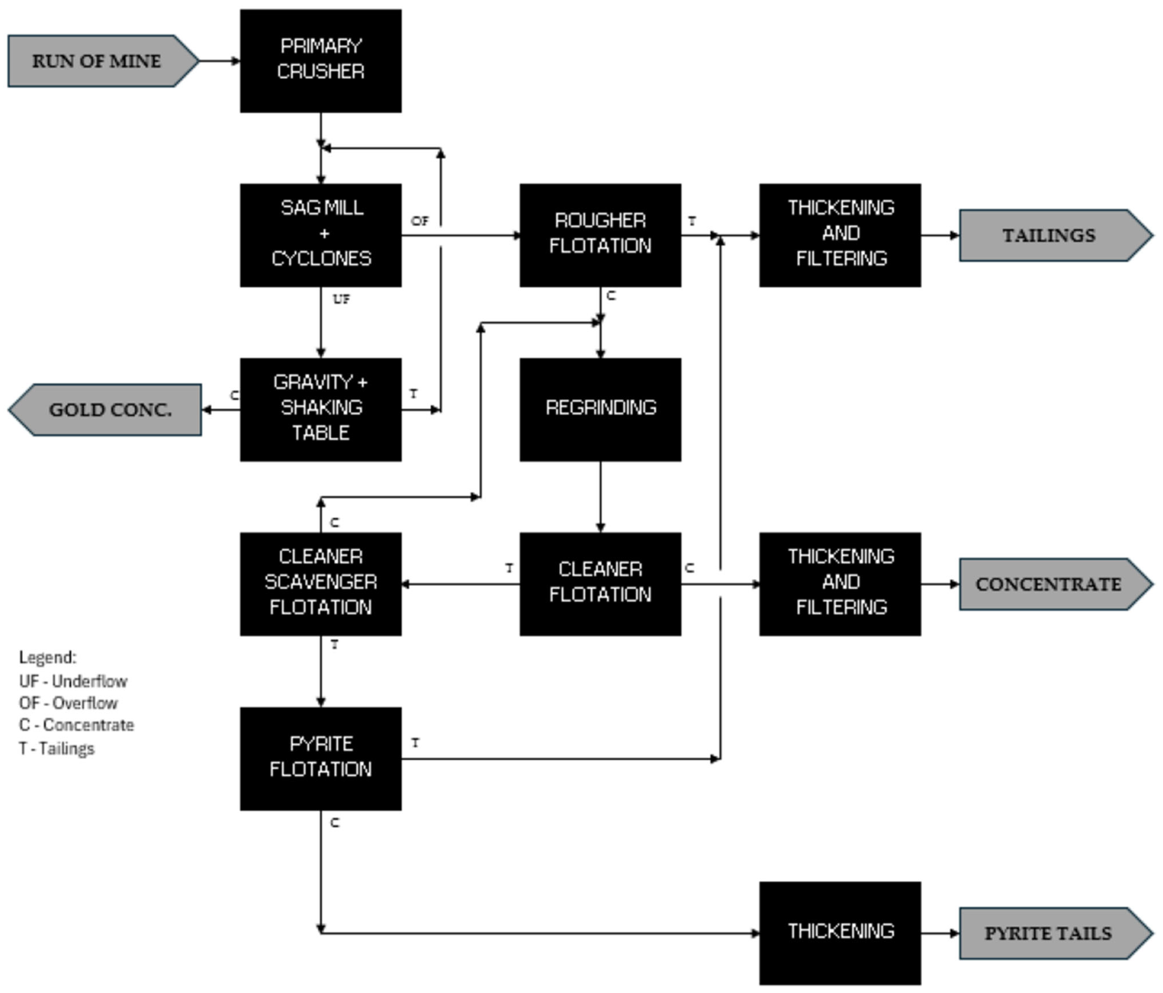
Based on the testwork results, the plant design includes primary jaw crushing, a grinding circuit with Semi-Autogenous Grinding (SAG) mill, and gravity-based gold re-covery. The flotation circuit utilizes rougher/scavenger tank cells and Jameson cleaner cells, with dewatering handled by thickening and filtering. Figure 3 presents the corre-sponding process block flow diagram.

2.5. Comminution Indices and Specific Energy

The Steve Morrell Comminution (SMC) methodology was applied to calculate the specific energy for each sample through the comminution indices obtained as results from the Drop Weight Test (DWT) and the Bond Ball Mill Work Index (BWI) test. Its use is related not only to the availability of databases to estimate comminution factors for the specific comminution energy but also to its widespread adoption in the industry [25,26,27,28].

2.5.1. SMC Parameters

The SMC Test® uses crushed rock fragments or particles originated from the cutting of drill core samples (“Cut-Core” method). The selected particles are fragmented using a rigorously controlled range of impact energies. The equipment used for the tests is the JK Drop Weight Tester, and the raw breakage data in these energy ranges are processed and generate the ore competency (toughness) parameters, in this case the breakage index (A*b). Other proprietary parameters are calculated based on the results of the SMC and Bond Ball Mill Work Index (BWI) tests, such as the Drop Weight Index (DWI), Mia (a parameter that describes the grinding of coarse material in tumbling mills), Mib (a parameter that describes the grinding of fine material in tumbling mills), Mic (a parameter that describes size reduction in crushing circuits), and Mih (a parameter that describes size reduction in high pressure grinding rolls circuits) [29]. Such values have good correlation indices with the A*b and BWI parameters and can also be estimated via correlation curves presented in Table 2.

2.5.2. Bond Ball Mill Work Index

The BWI test is performed under well-established standard conditions as: dry sample, with 700 mL volume and material below 3.35 mm particle size (or sieve size); use of a standardized mill, with dimensions 305 × 305 mm, standard speed of 70 rpm (91.4%); ball load with 285 steel spheres, following a standard size distribution; obtaining a stabilized circulating load of 250% [30].
The BWI for ball mills is calculated by Equation (1):
B W I = 44.5 P i 0.23 G b 0.82 ( 10 P 80 10 F 80 )   1.102
where BWI is the Bond Ball Mill work index for grinding in a ball mill (kWh/t); Pi is the aperture (µm) of the test’s classifying screen; P80 is the aperture (µm) of the sieve through which 80% of the product mass passes; F80 is the aperture (µm) of the sieve through which 80% of the feed mass passes, Gb is the average of the last three values of the grindability index at equilibrium state (g/rev) and 1.102 is short ton to metric ton conversion factor [30].

2.5.3. Mia and Mib

Table 2 presents the expressions used to calculate Mia and Mib, which are derived from established literature databases. The Mia calculation is based on item 1 where the correlation with A*b is presented. The Mib calculation is based on the expressions presented in items 2 to 5, based on their correlations with BWI. A key factor in selecting appropriate Mib curve selection is the reference product top size reference (ranging from 105 to 300 µm) [25,26]. In this study, a 300 µm top size was used, consistent with the target grinding circuit P80 of 212 µm.

2.5.4. Calculation of Specific Energy

For circuits with SAG mill and Ball mill (SABC Circuit), Morrell’s equations define the specific grinding energy (E) by the sum of the specific grinding energy for coarse fraction of the ore (Wa, P80 > 750 µm) and fine fraction (Wb, P80 < 750 µm). The specific comminution energy is estimated according to Equations (2)–(4).
E = W a + W b
W a = 4 M i a ( 750 ( 0.295 + 750 1 0 6 ) F 80 ( 0.295 + F 80 1 0 6 ) ) K 1
W b = 4 M i b ( P 80 ( 0.295 + P 80 1 0 6 ) 750 ( 0.295 + 750 1 0 6 ) )
where Mia is work index of the coarse ore fraction; F80 is 80% passing size of the fresh feed to the grinding circuit, in µm; K1 is Pebble grinding efficiency factor, being 0.95 when there is pebble recirculation and 1 when there is no pebble recirculation; Mib is work index of the fine ore fraction, calculated from the BWI, and P80 is 80% passing size of the fresh feed to the grinding circuit, in µm [31].

2.5.5. Block Throughput and Processing Time

The grinding throughput (t/h) is mapped for each block to be mined. This index is important because the existing capacity restrictions in the plant must be respected. This throughput is calculated as presented in Equation (5) [32].
T B l o c k = P E
where TBlock is the block’s throughput rate in the plant (t/h); P is the power available on the mills (kW); E is the specific energy of the ore (kWh/t).
The block processing time is calculated according to Equation (6). This time is important for the mining sequence, given that the sum of the processing time of the blocks planned to feed the processing plant must be limited to the total plant operational time for each period [32].
T P B l o c k = M B l o c k T B l o c k
where TPBlock is the block processing time in grinding (h); MBlock is the total mass of the block to be processed (t); PBlock is the block’s throughput in the plant (t/h).

2.6. Geometallurgy Modeling

Geometallurgical modeling relies on regression to predict metallurgical responses (dependent variables) using readily available ore characteristics (independent variables). Regression models were developed for the recoveries of copper, gold, and silver, specific comminution energy, and abrasion index (Ai). Such regressions are necessary due to the limited number of tests for the target variables in the project’s dataset, which does not allow the estimation of these variables by geostatistics methods, and the variability of these results in study dataset.

2.6.1. Specific Comminution Energy (E) Modeling

Direct modeling of Specific Comminution Energy was preferred over intermediate indices (A*b and BWI) because this approach reduces the mathematical biases introduced to final energy estimates. Such biases are related not only to the non-additivity of these variables with grades in the block model, but also to the staged calculation of this specific energy, which causes cumulative error in the specific energy estimate [33].

2.6.2. Abrasion Index (Ai) Modeling

With few results available (10 in total), the abrasion index regression modeling was made considering grades as proxies. No filter was applied to the dataset for this modelling.

2.6.3. Recovery (RCu, RAu, RAg) Modellings

Preliminary filtering was done on the dataset, considering the removal of samples qualified as “Low sulfur content” or “Biotite Rich”.
For context, low sulfur ores are related to materials ranging from average to high levels of weathering and sulfur grades less than 0.1%. Biotite-rich materials contain high grades in general but low recoveries. Both materials were tested for exploratory reasons. Proper testwork for them is planned to occur in the next phases of the reference project.
This filtering allowed the use of 19 samples in total to develop the grade-recovery models for each metal. Since these types of material represent a low percentage of the total ore (considered probable reserves, part of 11% of the total reserve), the grade-recovery modeling obtained for fresh feed (%S > 0.1) was considered valid at this level of study for this type of material.

2.7. Gold Equivalent Grade

To simplify complexity during mine sequencing for this polymetallic deposit, all metal grades were converted into a single measure: the gold equivalent grade (Au Eq). The gold equivalent grade calculation, presented in Equation (7), uses gold as the anchor element and incorporates the price and recovery of each contained element [22].
A u E q = t A u   R e c A u + i = 1 n c i   F i   t i   R e c i
where AuEq is the equivalent gold grade (ppm); tAu is the block gold grade; RecAu is the block gold recovery; i is the element or mineral of interest; n is the number of different elements or minerals considered in the calculation; ci is a multiplicative factor related to the units of grade relative to the reference grade (e.g., 10,000 is assumed if the grade is given in percentage and 1 if in ppm (g/t)); Fi is the quotient factor between the price of commodity i and the price of Gold; ti is the grade of element or mineral i; Reci is the recovery of element or mineral i.

2.8. Deposit’s Block Model

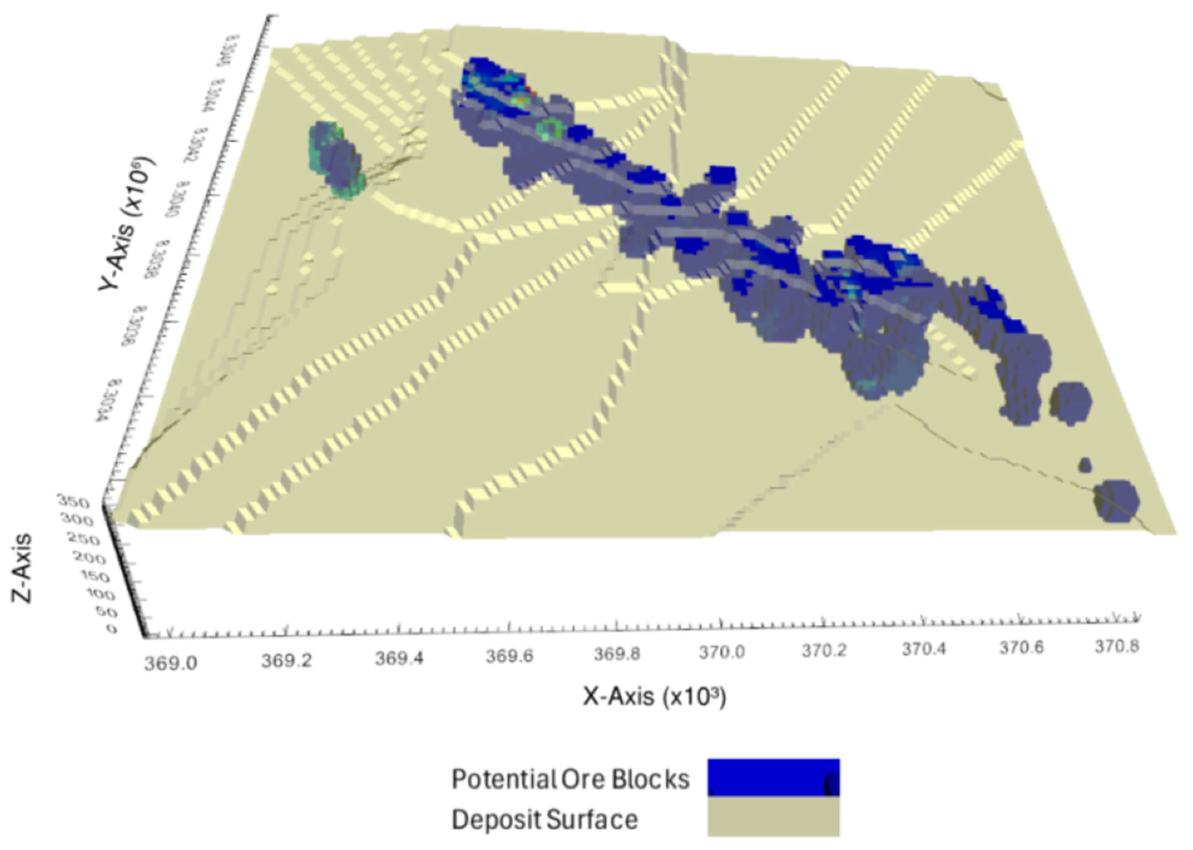
The block model of the deposit supplied for this study was built from 145 boreholes and 338 chemical samples. The spatial distributions of the boreholes and samples are presented in Figure 4. The block model is composed of 263,595 blocks, each measuring 15 × 15 × 15 m, and contains information for three grades: copper (Cu), gold (Au), and silver (Ag). The overall view of the block model is presented in Figure 5, where blocks with copper grades above 0.1% were used as a reference to show possible ore blocks within the deposit. The grade distribution within the block model is detailed in Figure 6, Figure 7 and Figure 8.

2.9. Block Value Calculations

2.9.1. Revenues

Revenues are calculated per block, based on the projected production and sales values of the commodities (cost of sale), as presented in Equation (8) [34].
R i = M i   P u n i t
where Ri is the projected revenue in block i for a specific product ($); Mi is the mass of product generated in the block i (t), and Punit is the unit price of the product ($/t).
For block revenue calculations, commodity prices are based on market values adopted at the Pre-Feasibility Study (PFS), while indices of refinery recoveries were based on the ratio between total costs for metals refining and the metals reference price. The values used are detailed in Table 3.

2.9.2. Operating Costs

Operating costs are related to mine activities, energy, material processing, and other cost components. Generally, specific costs per ton of moved ore are available, related to each item that makes up the operating cost of a mining venture. Each cost item is calculated according to Equation (9) [34].
C j = M b l o c k   C s p c
where Cj is the block cost in relation to a specific item, such as mine, energy, plant, transport, penalties, and others ($); MBlock is the mass of the block (t), and Cspc is the specific cost related to a specific operating cost item ($/t).
Each specific cost considered for this study was based on the original PFS operating cost (OPEX) estimate. Portions of fixed and variable costs considered for this study are presented in Table 4.

2.9.3. Block Value

The actual block value consists of the difference between block revenues and expenses, as presented in Equation (10).
V b = i = 1 n R i j = 1 m C j
where Vb is the value of block b; n is the number of revenue-generating products predicted in the project (commodities/co-products); m is the number of different cost items existing in the analysis; Ri is the projected revenue in the block for a specific product i ($) and; Cj is the cost of the block in relation to a specific item j ($).

2.10. Direct Block Sequencing

Direct Block Sequencing (DBS) is a mining optimization technique that belongs to the category of integer programming algorithms. Different from classical methods that divide the problem into two stages, determining the ultimate pit limit and scheduling, DBS seeks to integrate these decisions into a single stage (global optimization).
The technique formulates the mine planning problem as a non-linear (or linearized) integer problem, where binary decision variables indicate whether a given block will be mined in a specific period or not. The main objective is to maximize the Net Present Value (NPV) of the mine, respecting all geometric, metallurgical, and productive capacity constraints over time [35].
DBS is notable for its ability to generate economically optimal mining sequences without depending on a predefined pit limit, producing results that often surpass those obtained by two-stage approaches [35]. In the literature, DBS is known as the Precedence Constrained Production Scheduling Problem (PCPSP) [36], or the Production Scheduling Problem with Precedence Constraints. In the PCPSP, the economic value of a block can be calculated according to its destination, for example, a processing plant or a waste pile, using Equations (11) and (12).
P r o c e s s = M B   g   r ( S P S c ) M B ( C P + C M )
W a s t e = M B C M
where MB is the block mass (t); g is the grade; r is the recovery; Sp is the sale price ($); Sc is selling cost; CP is the block processing cost ($); CM is the block mining cost ($).
The optimization algorithm selects the best destination for each block based on its value. In this approach, it is not necessary to define cut-off grades or predetermine whether a block is classified as ore or waste before optimization. MiningMath (MM) software was used in this study. Figure 9 shows the simplified flowchart of the MiningMath algorithm [37].
The first step of the optimization algorithm is to remove regions that do not add any value to the project. The second stage of the optimization algorithm consists of converting the non-linear integer problem into a linear problem based on surfaces (geometric mine constraints). These constraints are BW (represents the bottom width), MW (related to mining width), and ADV (vertical rate of advance).
The third step of the optimization algorithm consists of converting the linear solution into an integer solution using the branch-and-cut algorithm [38]. This algorithm is more efficient than the branch-and-bound algorithm [39], contained in standard Mixed Integer Linear Programming (MILP) solvers [40,41], and was even specifically tuned for this optimization problem.

2.10.1. Mine Scheduling Scenarios

In this research, a total of 8 geometallurgical block models were developed. These models were differentiated by the number of geometallurgical variables considered in the calculation of the blocks’ economic value. Fixed and variable conditions for each scenario consider the possible application of regression models and proportion calculations related to each block characteristic. In terms of complexity, scenario 1 was the least complex scenario, with a zero level of geometallurgical modeling (in other words, all key geometallurgical variables had values fixed within blocks), while scenario 8 was the most complex scenario, with all variables modeled within blocks. The differences and criteria for these 8 scenarios are presented in Table 5 and Table 6. Key mine scheduling inputs were kept consistent across all scenarios as presented in Table 7.
Fixed and variable costs, explained previously in Table 4 and detailed in Table 6 for mining, consumables, and energy costs, are based on the original PFS OPEX estimate. In the variable condition column, the cost is divided into a fixed portion (usually a flat number) and a variable portion (linked to a specific block property).
The key sequencing inputs presented in Table 7 are based on the original PFS results. Maximum gold equivalent grade and process plant throughput are directly correlated to the original plant design for phase 1 of the concentrator. Slope angles and the maximum annual vertical advance rate are based on the mining concept adopted in the PFS mining development. A discount rate of 8% was based on the real interest rate in Brazil at the time of the study (developed in April 2025) [42].

2.10.2. Software Used

For the development of the scenarios, the MiningMath software, version v3.0.33, was used to perform the mine sequencing via the DBS algorithm.

3. Results and Discussion

3.1. Specific Comminution Energy

Additionally, to the results presented in Table 1, the specific comminution energy (E) was calculated according to SMC (Equations (2)–(4)) for each sample before the development of regression modeling. The results of this calculation are presented in Figure 10. The total variation captured in specific comminution energy between samples was 16.07 kWh/t, that is 14.0% higher than the reference specific energy adopted for the project (14.1 kWh/t). This level of variation demonstrated the importance of modeling the specific comminution energy for this deposit.

3.2. Regression Models

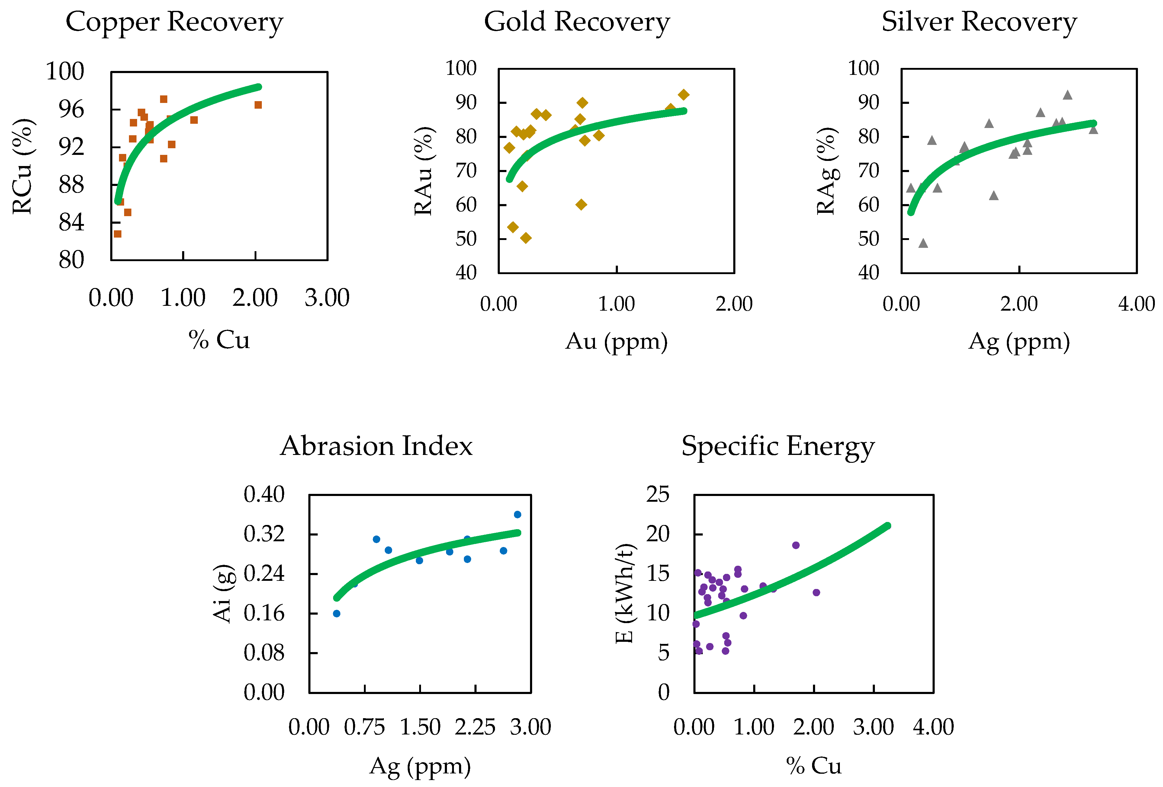
The regression models for each geometallurgy variable are presented in Figure 11. Equations with coefficient of determination (R2) are presented in Table 8.
Although the low R2 values (with all results below 0.65) indicate that the regression models represented only a moderate portion of the total metallurgical variability, the resulting curves were considered useful for the context of geometallurgical modeling in this initial stage of the project (limited data). The utility was confirmed by visual evaluation, where the estimated curve aligned with the general distribution of the data, particularly in regions of higher sample density. Figure 12 presents a visual representation of how variability is captured when comparing the results from regression against a fixed number (red line in the middle of the graph) for specific comminution energy in this dataset. Comparative analysis of the Chi-squared residuals x2) presented in Table 9 indicates that the regression curves yield a more robust goodness of fit than the fixed or optimized fixed indices [43]. Although the R2 values remain low, suggesting limited explanatory power, the minimized x2 values for the regression results demonstrate a higher degree of statistical alignment with the observed data compared to all fixed-value configurations.
For the specific energy and abrasion index, the use of grades (copper, gold, and silver) as independent variables was necessary, since these were the only information available in the provided block model. This data limitation forced reliance on grades as the only available proxies to estimate and populate the specific energy and abrasion index in the ore blocks. This approach was employed despite the understanding that rock properties, such as grain size, interlocking, drill penetration rate, and oxidation state, are superior variables for capturing the true trend of comminution indices [44].
The incorporation of the regression-predicted values in the geometallurgical block models followed the restrictions in Table 10. These conditions are indispensable to ensure the physical validity and mathematical coherence of the results (avoiding, for example, recoveries greater than 100% or negative indices), in addition to maintaining the adherence of the maximum and minimum block values to the distribution of maximum and minimum values of the filtered dataset for all variables.

3.3. Mine Scheduling Results

Each of the 8 scenarios studied (detailed in Table 5 and Table 6), generated a block model, that was used to run mine scheduling by DBS (detailed in Table 7) to calculate deposit’s NPV and mining sequence technical aspects (such as plant feed, waste, global mass movement and others). Figure 13 and Figure 14 present summaries of technical and economic results for all scenarios.
In terms of plant feed, the simulations demonstrated long-term stability in the total plant processing capacity. The total Run-of-Mine (ROM) mass processed varied minimally, with a point difference of 65.3 to 69.5 Mt between the minimum and maximum scenario, but with a variation around the average between scenarios slightly above 2.0%. These differences were mainly attributable to small variations in the Life of Mine (LOM) duration (27 to 29 years). All scenarios consistently achieved the annual design capacity of 2.50 Mt/a in over 60% of the total production period, with average annual production rates showing a minimal difference of 0.12 Mt (2.30 Mt to 2.42 Mt). Therefore, the increase in the number of variables in geometallurgical modeling did not significantly affect the total quantities of ROM production.
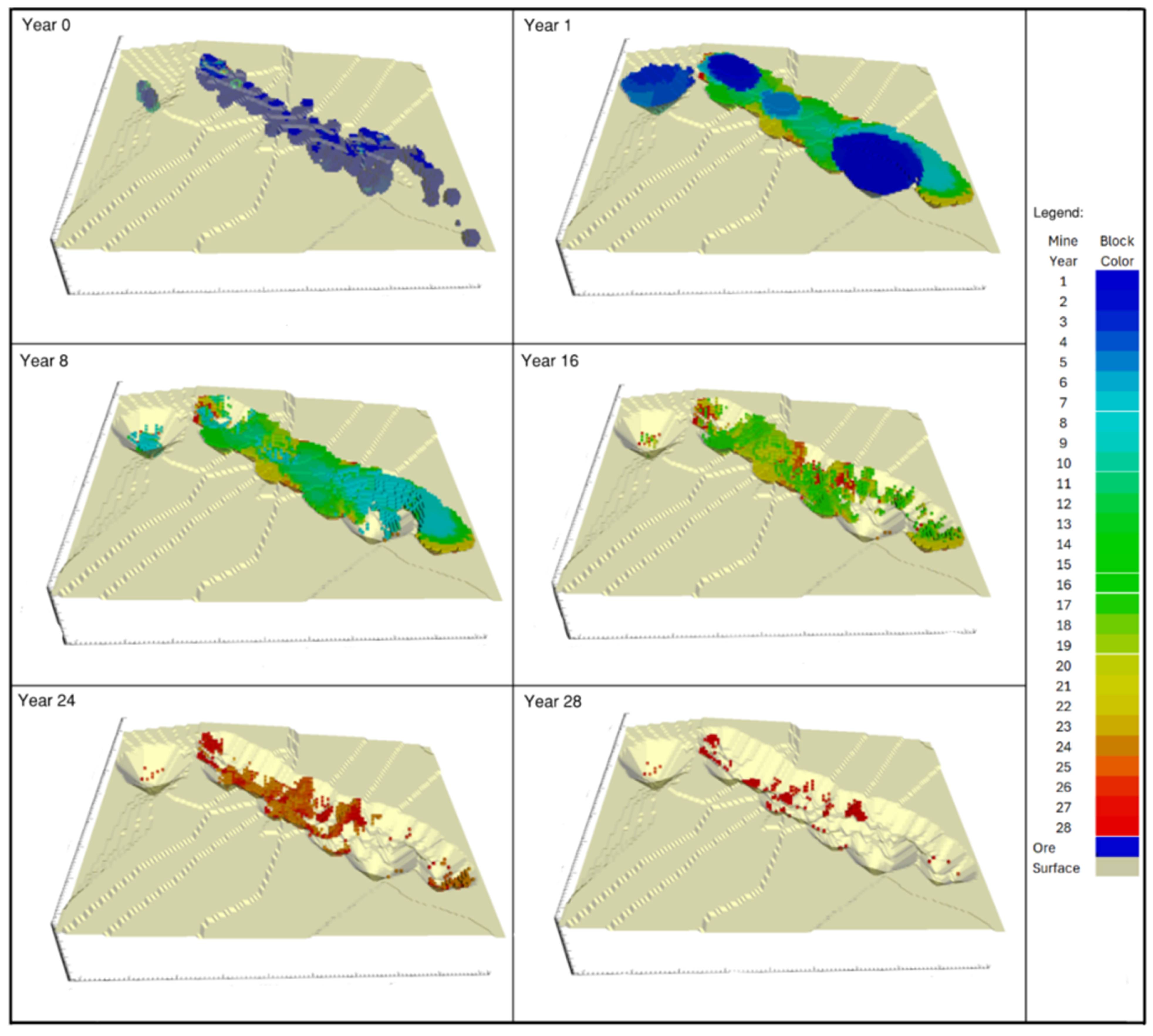
The total production of waste exhibited high consistency (approx. 1.35% variation relative to the average around 99 Mt). Therefore, similar to plant feed results, the increase in variables in geometallurgical modeling did not significantly affect the total generation of waste and global material movement. The final shape of the open pit, after the production years of each scenario, was similar. Figure 15 presents the open pit shape for Scenario 8 in years 0, 1, 8, 16, 24, and 28.
Regarding processing time, the average values (5567 h to 5881 h) and the maximum time reached (6687 h to 6987 h) varied slightly and remained significantly below the projected limit of 8059 h. This observation suggested that the greater complexity of the modeling allowed for the understanding that the SAG mill is potentially oversized. A possible reduction of 13.3% in the necessary comminution energy (based on the difference between the design and the maximum processing time reached) must be investigated in the next steps of the study, with a reinforced dataset, to avoid potential extra capital expenditure in project implementation.
The total equivalent gold production showed significant sensitivity to the model complexity, with an overall maximum difference of 1.36 t between Scenario 1 (31.55 t) and Scenarios 5 and 8 (32.92 t), representing a notable increase of 4.31%. The results indicated that the gold recovery and mine cost variables were the ones that most affected the total equivalent gold result. Since the main geometallurgical factors (mine cost, variable gold recovery, and variable copper recovery) were adequately represented, there were practically no gains in equivalent gold production, as can be observed when comparing the results between scenarios 5 and 8. The other variables added to the geometallurgical model (e.g., variable consumption/energy costs) did not necessarily result in production improvements but were optimal for indicating a tendency towards stability in the equivalent gold production value.
Figure 14 and Figure 16 show that NPV varied 6.92% between the lowest result (Scenario 1) and the highest (scenarios 5 and 8), highlighting its importance as a decision metric. A distinct pattern emerged between scenarios 1 and 5, where there was a significant difference in NPV, confirming that the application of high impact variables (in this study, variations caused by mine cost at +4.24%, gold recovery at +3.61% and copper recovery at −1.21%) was extremely beneficial to the project’s economics. Between scenarios 5 and 8, a tendency towards NPV stability was noted, with the positive and negative oscillations between these scenarios consistently below 0.6%, indicating that the increase in the number of variables brought stability to the economic results, presenting a trend NPV value between 1680 and 1690 M USD.

4. Conclusions and Recommendations

This study presented and discussed the geometallurgical approach applied in an early-stage project context with limited data. For the deposit under study, by demonstrating the potential positive 6.92% variation in NPV between scenarios, the research confirmed not only the hypothesis of geometallurgy’s positive impact on NPV, but also the importance of geometallurgical modeling even when data are initially scarce.
Although the results of the regression models were considered weak (low R2 values), the results of this exercise remain important, as the geometallurgical approach for this polymetallic deposit supported the mitigation of potential technical risks, such as potential equipment oversize, ore bottlenecks, and excess consumable costs. Also, economic risks such as optimistic/unreal capital expenditure (CAPEX) and operating cost (OPEX) estimates can be mitigated at a low cost of opportunity (less than 1% of total OPEX per year, considering a conservative estimate for a more robust dataset).
From the results, it was concluded that more variables in geometallurgical modeling can affect the overall economic results of the deposit, depending on the impact these variables have on the NPV estimation:
  • High-impact variables, when well-modeled, show real NPV potential. For the deposit studied, the variables gold recovery, mine costs, and copper recovery were considered high-impact and responsible for the largest NPV variations obtained.
  • Low-impact variables, such as specific comminution energy and abrasion index (related to energy and consumable costs), showed small variations (positive and negative, less than 0.6%) in deposit NPV. Although they did not contribute significantly to the deposit NPV, they were important for (1) identifying NPV stability and trend, and (2) understanding key technical points of the project, such as the potential for equipment selection improvements (e.g., specific energy vs. SAG power) and the understanding that processing time and overall processing plant capacity theoretically will not be exceeded.
The hypothesis that the adoption of more variables in geometallurgical modeling would not necessarily affect the technical aspects of deposit mine sequencing was confirmed. In our case, the quantities of material moved and the deposit’s production years were minimally affected by this increase.
The recommended approach is to develop geometallurgical models with the maximum number of variables possible, as this will allow mapping both the economic and technical aspects of the project that are well-consolidated or demand attention. In the next phases of the project, to achieve an adequate level of modeling and accurate answers, the use of a robust deposit dataset is recommended. It will assist in obtaining greater statistical robustness of the underlying geometallurgy models (R2 indices are currently below 0.65), through a greater number of tests and more detailed technical information on the deposit, such as mineralogical composition and sample positioning, among others.

Author Contributions

Conceptualization: L.F.d.S. and D.B.M.; methodology: L.F.d.S. and D.B.M.; formal analysis: L.F.d.S.; investigation. L.F.d.S.; writing—original draft preparation: L.F.d.S.; writing—review and editing: L.F.d.S., D.B.M., L.J.F.C. and K.C.F. All authors have read and agreed to the published version of the manuscript.

Funding

This research received no external funding.

Data Availability Statement

Data used to perform this research is publicly available.

Acknowledgments

MiningMath for software license, and UFMG Geometallurgy Lab team for the support.

Conflicts of Interest

The authors declare no conflicts of interest.

References

  1. Silva, R.d.C.; Ayres da Silva, A.L.M. Assessing Mining Performance Indicators in Relation to the SDGs: Development of a Guided Methodology and Its Application in an Iron Ore Mine. Minerals 2024, 14, 887. [Google Scholar] [CrossRef]
  2. International Energy Agency. The Role of Critical Minerals in Clean Energy Transitions; International Energy Agency: Paris, France, 2022; 283p. [Google Scholar]
  3. Dominy, S.C.; O’Connor, L.; Glass, H.J.; Xie, Y. Geometallurgical Study of a Gravity Recoverable Gold Orebody. Minerals 2018, 8, 186. [Google Scholar] [CrossRef]
  4. Lishchuk, V.; Koch, P.-H.; Ghorbani, Y.; Butcher, A.R. Towards integrated geometallurgical approach: Critical review of current practices and future trends. Minerals 2020, 10, 145. [Google Scholar] [CrossRef]
  5. Liebezeit, V.; Ehrig, K.; Robertson, A.; Grant, D.; Smith, M.; Bruyn, H. Embedding geometallurgy into mine planning practices—Practical examples at Olympic Dam. In Proceedings of the Third AusIMM International Geometallurgy Conference 2016, Perth, Australia, 15–17 June 2016; pp. 135–144. [Google Scholar]
  6. Bueno, M.; Foggiatto, B.; Lane, G. Geometallurgy Applied in Comminution to Minimize Design Risks. In Proceedings of the 6th International Conference on Semi-Autogenous and High-Pressure Grinding Technology (SAG 2015), Vancouver, BC, Canada, 20–24 September 2015; SAG Conference Foundation: Vancouver, Canada, 2015; pp. 1–19. [Google Scholar]
  7. Mu, Y.; Salas, J.C. Data-Driven Synthesis of a Geometallurgical Model for a Copper Deposit. Processes 2023, 11, 1775. [Google Scholar] [CrossRef]
  8. Supajaidee, N.; Chutsagulprom, N.; Moonchai, S. An Adaptive Moving Window Kriging Based on K-Means Clustering for Spatial Interpolation. Algorithms 2024, 17, 57. [Google Scholar] [CrossRef]
  9. Konishi, T. Means and Issues for Adjusting Principal Component Analysis Results. Algorithms 2025, 18, 129. [Google Scholar] [CrossRef]
  10. Silva, P.; Hidalgo, M.; Hotchkiss, M.; Dharmasena, L.; Linkov, I.; Fiondella, L. Predictive Resilience Modeling Using Statistical Regression Methods. Mathematics 2024, 12, 2380. [Google Scholar] [CrossRef]
  11. Bergholz, W.S.; Schreder, M.L. Escondida—Phase IV Grinding Circuit. In Proceedings of the 36th Annual Meeting, Montreal, QC, Canada, 20–22 January, 2004; The Canadian Institute of Mining, Metallurgy and Petroleum: Westmount, QC, Canada, 2004; pp. 1–16. [Google Scholar]
  12. Amelunxen, P.; Mular, M.A.; Vanderbeek, J.; Hill, L.; Herrera, E. The effects of ore variability on HPGR trade-off economics. In Proceedings of the International Autogenous and Semi-autogenous Grinding and High-Pressure Grinding Roll Technology 2011, Vancouver, BC, Canada, 25–28 September 2011; Major, K., Flintoff, B.C., Klein, B., McLeod, K., Eds.; University of British Columbia (UBC): Vancouver, BC, Canada, 2011. [Google Scholar]
  13. Wirfiyata, F.; McCaffery, K. Applied geo-metallurgical characterization for life of mine throughput prediction at Batu Hijau. In Proceedings of the International Autogenous and Semi-autogenous Grinding and High-Pressure Grinding Roll Technology 2011, Vancouver, BC, Canada, 25–28 September 2011; Major, K., Flintoff, B.C., Klein, B., McLeod, K., Eds.; University of British Columbia (UBC): Vancouver, BC, Canada, 2011. [Google Scholar]
  14. Keeney, L.; Walters, S.G. A Methodology for Geometallurgical Mapping and Orebody Modelling. In Proceedings of the First AusIMM International Geometallurgy Conference 2013, Brisbane, Australia, 30 September–2 October 2013; Dominy, D., Ed.; Australasian Institute of Mining and Metallurgy (AusIMM): Carlton, Australia; pp. 217–225. [Google Scholar]
  15. da Mata, J.F.C.; Nader, A.S.; Mazzinghy, D.B. Inclusion of the geometallurgical variable specific energy in the mine planning using direct block scheduling. Tecnol. Metal. Mater. Min. 2022, 19, e2677. [Google Scholar] [CrossRef]
  16. da Mata, J.F.C.; Nader, A.S.; Mazzinghy, D.B. Methodology to include the comminution specific energy into open-pit strategy mine planning using global optimization. Tecnol. Metal. Mater. Min. 2022, 19, e2752. [Google Scholar] [CrossRef]
  17. Mata, J.F.C.D.; Nader, A.S.; Mazzinghy, D.B. A Case Study of Incorporating Variable Recovery and Specific Energy in Long-Term Open Pit Mining. Mining 2023, 3, 367–386. [Google Scholar] [CrossRef]
  18. Martins, S.; Campos, P.; Mazzinghy, D.B. A case study comparing the results of a copper open-pit mine scheduling considering two different approaches for spatial interpolation of comminution geometallurgical variables. J. Sustain. Min. 2025, 24, 472–485. [Google Scholar] [CrossRef]
  19. Rangel, L.V.; Mazzinghy, D.B.; da Silva, G.R.; Seguin, F.; Teixeira, M.F.D.L.; Junior, S.U.F.; Vieira, C.H.R.; Junior, W.F.B.; Silva, V.C.; Dimitrov, G.R. Geometallurgy study of the Catalão I Nelsonite bodies aiming to increase the niobium production. Tecnol. Metal. Mater. Min. 2020, 17, e2214. [Google Scholar] [CrossRef]
  20. Käyhkö, T.; Sinche-Gonzalez, M.; Khizanishvili, S.; Liipo, J. Validation of predictive flotation models in blended ores for concentrator process design. Miner. Eng. 2022, 185, 107685. [Google Scholar] [CrossRef]
  21. Raponi, T.R.; Elfen, S.C.; Tear, S.; McCartney, J.A.; Soares, L.; Lotter, N.; Lima, J.F.; Rodriguez, P.C. Cabaçal Gold-Copper Project. NI 43-101 Technical Re-Port and Pre-Feasibility Study. 2025. Available online: https://wp-meridianmining-2023.s3.ca-central-1.amazonaws.com/media/2025/04/Cabacal-Project-NI-43-101-Technical-Report-and-PFS_FINAL.pdf (accessed on 1 November 2025).
  22. Raponi, T.R.; Elfen, S.C.; Tear, S.; Batelochi, M.; Keane, J.; Ferreira, G.G. Cabaçal Gold-Copper Project. NI 43-101 Technical Report and Preliminary Economic Assessment. 2023. Available online: https://meridianmining.co/wp-content/uploads/2023/03/Cabacal-NI_43-101-Technical-Report_Final.pdf (accessed on 1 November 2025).
  23. Dominy, S.C.; Glass, H.J. Geometallurgical Sampling and Testwork for Gold Mineralisation: General Considerations and a Case Study. Minerals 2025, 15, 370. [Google Scholar] [CrossRef]
  24. Bond, F.C. Metal Wear in Crushing and Grinding. Chem. Eng. Prog. 1964, 60, 111–114. [Google Scholar]
  25. Doll, A. SMC Test Parameters from BWI. LinkedIn. 2022. Available online: https://ca.linkedin.com/posts/alex-doll-66b57465_workindex-comminution-activity-6935422189697470464-JLCm (accessed on 26 December 2023).
  26. Doll, A. SMC Test Parameters from A × b. LinkedIn 2024. Available online: https://www.linkedin.com/posts/alex-doll-66b57465_comminution-grindability-smctest-activity-7152238024792121344-7hB0 (accessed on 18 January 2024).
  27. Morrell, S. Global Trends in Ore Hardness. In Proceedings of the SAG Conference 2015, Vancouver, BC, Canada, 20–24 September 2015; pp. 1–22. [Google Scholar]
  28. Morrell, S. The Morrell Method for Determining Comminution Circuit Specific Energy and Assessing Energy Utilization Efficiency of Existing Circuits. Miner. Eng. 2009, 22, 416–424. [Google Scholar]
  29. Morrell, S. An alternative energy–size relationship to that proposed by Bond for the design and optimisation of grinding circuits. Int. J. Miner. Process. 2004, 74, 133–141. [Google Scholar] [CrossRef]
  30. Bond, F.C. Crushing and grinding calculations. Min. Eng. 1959, 11, 548–554. [Google Scholar]
  31. Morrell, S. Predicting SAG/AG Mill and HPGR Specific Energy Requirements Using the SMC Rock Characterisation Test. In Proceedings of the Randol Gold & Silver Forum, Vancouver, BC, Canada, 12–15 September 2004; Randol International: Perth, Australia, 2004; pp. 1–10. [Google Scholar]
  32. Mazzinghy, D.B.; Morales, N.; Brickey, A.; Nelis, G.; Ortiz, J.; Souza, M.J.F. Mineral processing plant capacity based on geometallurgical block model scheduling. In Proceedings of the APCOM Conference 2025: Application of Computers and Operations Research in the Minerals Industry, Perth, Australia, 10–13 August 2025; The Australasian Institute of Mining and Metallurgy (AusIMM): Carlton, VIC, Australia, 2025; pp. 755–770, ISBN 978-1-922395-50-4. [Google Scholar]
  33. Sepulveda, E.; Dowd, P.A.; Xu, C.; Addo, E. Multivariate Modelling of Geometallurgical Variables by Projection Pursuit. Math. Geosci. 2017, 49, 121–143. [Google Scholar] [CrossRef]
  34. Silva, L.F.; Magalhães, L.F.; Campos, L.J.F.; Mazzinghy, D.B. Abordagem geometalúrgica aplicada a um novo depósito polimetálico de cobre, ouro e prata na região Centro Oeste do Brasil. In Proceedings of the Anais do 1º Simpósio de Geometalurgia, Belo Horizonte, Brazil, 24–25 June 2024; UFMG: Belo Horizonte, Brazil, 2024; pp. 97–107. [Google Scholar]
  35. Johnson, T.B. Optimum open pit mine production scheduling. Ph.D. Thesis, Operations Research Department, University of California, Berkeley, CA, USA, 1968. [Google Scholar]
  36. Espinoza, D.; Goycoolea, M.; Moreno, E.; Newman, A. MineLib: A library of open pit mining problems. Ann. Oper. Res. 2012, 206, 91–114. [Google Scholar] [CrossRef]
  37. MiningMath®. MiningMath’s Knowledge Base. 2021. Available online: https://knowledge.miningmath.com/ (accessed on 14 November 2025).
  38. Song, Y.; Zhang, Y. A Branch-and-Price-and-Cut Algorithm for the Inland Container Transportation Problem with Limited Depot Capacity. Appl. Sci. 2024, 14, 11958. [Google Scholar] [CrossRef]
  39. He, H.; Zhao, Y.; Ma, X.; Lv, Z.-G.; Wang, J.-B. Branch-and-Bound and Heuristic Algorithms for Group Scheduling with Due-Date Assignment and Resource Allocation. Mathematics 2023, 11, 4745. [Google Scholar] [CrossRef]
  40. Jelvez, E.; Ortiz, J.; Varela, N.M.; Askari-Nasab, H.; Nelis, G. A Multi-Stage Methodology for Long-Term Open-Pit Mine Production Planning under Ore Grade Uncertainty. Mathematics 2023, 11, 3907. [Google Scholar] [CrossRef]
  41. François, C.; Ljubić, I. Last fifty years of integer linear programming: A focus on recent practical advances. Eur. J. Oper. Res. 2025, 324, 707–731. [Google Scholar] [CrossRef]
  42. Veloso, V. Veja Qual é a Taxa Selic Hoje (Abril de 2025). Portal AECweb. 2025. Available online: https://www.aecweb.com.br/revista/noticias/qual-taxa-selic-hoje-esse-mes/24908 (accessed on 18 December 2025).
  43. Espínola, F.; Castillo, E.; Orellana, L.F. Bibliometric and PESTEL Analysis of Deep-Sea Mining: Trends and Challenges for Sustainable Development. Mining 2025, 5, 36. [Google Scholar] [CrossRef]
  44. Bhuiyan, M.; Esmaieli, K.; Ordóñez-Calderón, J.C. Application of Data Analytics Techniques to Establish Geometallurgical Relationships to Bond Work Index at the Paracutu Mine, Minas Gerais, Brazil. Minerals 2019, 9, 302. [Google Scholar] [CrossRef]
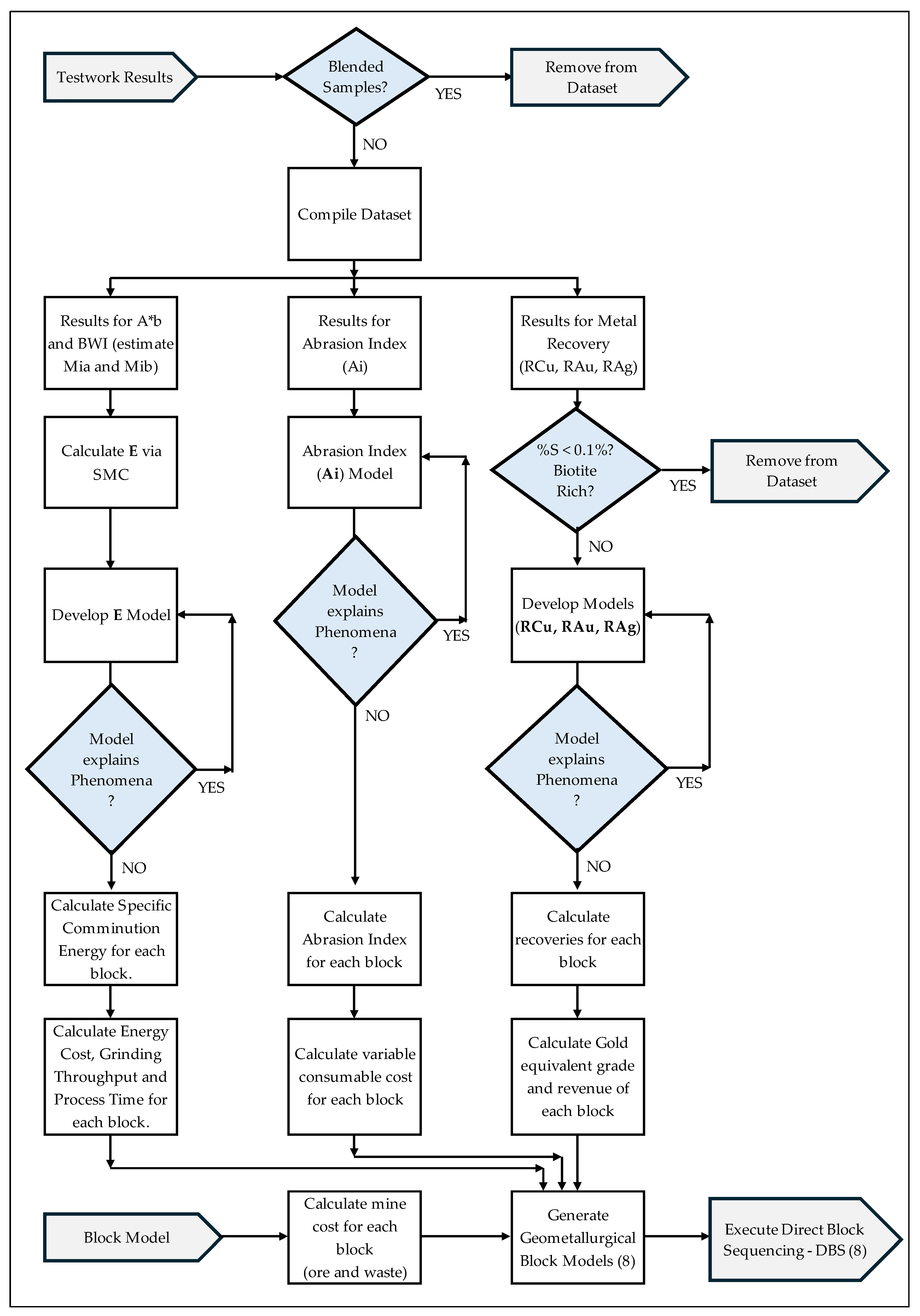
Figure 1. Study Methodology.
Minerals 16 00040 g001
Figure 2. Testwork samples spatial positioning in the reference project.
Minerals 16 00040 g002
Figure 3. Process Plant Block Flow Diagram.
Minerals 16 00040 g003
Figure 4. Spatial Distribution of Boreholes and Grades.
Minerals 16 00040 g004
Figure 5. Block model.
Minerals 16 00040 g005
Figure 6. Distribution—Copper grades.
Minerals 16 00040 g006
Figure 7. Distribution—Gold grades.
Minerals 16 00040 g007
Figure 8. Distribution—Silver grades.
Minerals 16 00040 g008
Figure 9. MiningMath Algorithm.
Minerals 16 00040 g009
Figure 10. Results—Specific Comminution Energy.
Minerals 16 00040 g010
Figure 11. Regression models (RCu, RAu, RAg, Ai, E).
Minerals 16 00040 g011
Figure 12. Comparison between fixed-value and model results for E in reference dataset.
Minerals 16 00040 g012
Figure 13. Mine scheduling technical results.
Minerals 16 00040 g013
Figure 14. Mine scheduling economic results.
Minerals 16 00040 g014
Figure 15. Open Pit Shapes for Scenario 8—Years 0, 1, 8, 16, 24, 28.
Minerals 16 00040 g015
Figure 16. Deposit NPV variation vs. Scenarios.
Minerals 16 00040 g016
Table 1. Testwork results.
Sample NameFeed GradesComminution IndicesRecoveriesDetail
CuAuAgA*bBWI AiCuAuAg
%ppmppm-kWh/tg%%%
CCZ-11.151.572.6339.211.20.2994.992.484.1
CCZ-20.220.090.6141.78.10.229076.865.1
CCZ-30.540.651.0747.69.80.2994.48277.3
ECZ-10.730.241.935.815.20.2990.874.575
ECZ-20.460.152.8242.99.70.3695.281.692.4
SCZ-10.230.270.374580.1685.181.948.9
SCZ-20.540.732.14339.70.2792.878.978.4
CNWE-10.310.40.9142.412.50.3194.686.473.1
CNWE-20.821.462.1468.711.40.319588.276.2
Zn Comp0.840.261.4945.513.70.2792.381.284
CAB-S10.520.851.57112.73.6-93.680.462.9
CAB-S20.530.21.0684.26.3-94.265.576.7
CAB-S30.130.70.3337.97.9-86.260.165.2
CAB-S40.160.690.5239.110.7-90.985.279.1
CAB-S50.230.380.4832.910.6-93.880.277.1Low S
CAB-S60.483.662.2340.711-95.365.271.7Low S
CAB-S70.060.370.633.311.9-79.866.817Low S
CAB-S80.420.212.7339.512.9-95.780.784.4
CAB-S90.730.322.3635.813.4-97.186.787.2
CAB-S110.040.770.53105.86-2.869.36.1Low S
CAB-S120.560.481.18102.56.1-46.954.539.4Low S
CAB-S130.081.690.72117.14.1-2.783.429.8Low S
CAB-S160.260.350.76123.66.8-21.17232Low S
CAB-S171.70.7810.0232.721.5-75.356.955Biotite Rich
CAB-S183.230.8516.2828.324.1-71.955.266.3Biotite Rich
CAB-S190.090.230.1648.994 82.850.365.1
CAB-S202.040.713.2641.810.3-96.59082.2
CAB-S210.033.380.6260.75.5-48.574.818.5Low S
CAB-S220.30.121.9434.39.9-92.953.575.7
Table 2. Equations correlating Mia and Mib with comminution indices.
ItemVariableEquationDetails
1Mia M i a = 379.40   A b 0.80 R2 = 1.00
2Mib M i b = 0.71   B W I 1.24 P100 = 105 µm
3 M i b = 0.69   B W I 1.22 P100 = 150 µm
4 M i b = 0.63   B W I 1.21 P100 = 212 µm
5 M i b = 0.60   B W I 1.20 P100 = 300 µm
Table 3. Assumptions for block revenue calculations.
ItemValueUnit
* Gold Price68,129.83USD/kg
* Copper Price9.17USD/kg
* Silver Price864.85USD/kg
** Recovery—Cu Refinery96.30%
** Recovery—Au Refinery96.60%
** Recovery—Ag Refinery90.00%
* Reference—November 2024, considering consensus from various financial institutions. ** Indices based on refining costs.
Table 4. Specific Operating Costs (OPEX).
ItemFixed CostVariable CostDetails
Mining (Ore and waste costs)Drilling, Blasting, Load, Scattering (if applicable)TransportTransport cost for ore and waste varies according to Block’s height in relation to process plant.
Power CostOverall Plant (excluding comminution)ComminutionVariable cost based on Specific Comminution Energy for each block.
Reagents CostAll reagentsNot applicableNot applicable in this study
Consumable CostFiltering clothesLiners for Crushers and Mills, Grinding Media.Consumable cost varies according to Abrasion Index for each block.
Other itemsLabour, Maintenance, Water/Sewage, Access Maintenance, Laboratory, Dry Stacking, General and Administrative (G&A), Concentrate LogisticsNot applicableAs per the original estimate in deposit’s PFS.
Table 5. Scenarios description.
ScenarioMaximum Block Process TimeMine CostRecoveriesConsumables CostEnergy Cost
1VariableFixedAll FixedFixedFixed
2FixedFixedAll FixedFixedFixed
3FixedVariableAll FixedFixedFixed
4FixedVariableCu—Variable
Au—Fixed
Ag—Fixed
FixedFixed
5FixedVariableCu—Variable
Au—Variable
Ag—Fixed
FixedFixed
6FixedVariableAll VariableFixedFixed
7FixedVariableAll VariableVariableFixed
8FixedVariableAll VariableVariableVariable
Table 6. Scenarios criteria.
Geometallurgy
Variable
Fixed ConditionVariable Condition
* Block Process Time8059 h per year maxNot limited
Mine CostOre = 3.63 USD/tOre = 2.26 + 0.005464 ∗ (357.5 − Z) USD/t
Waste = 3.61 USD/tWaste = 2.29 + 0.004972 ∗ (357.5 − Z) USD/t
Recoveries75th percentile from testwork results
Cu Recovery = 94.75%
Au Recovery = 81.95%
Ag Recovery = 78.75%
As per regression models for each metal
Consumables Cost1.93 USD/t ore(0.73 + 1.20 ∗ Block Ai/0.281) USD/t ore
Energy Cost2.31 USD/t(1.29 + specific energy ∗ 0.072) USD/t ore
* Restriction related to mill operating availability of 92% as defined in plant design.
Table 7. Direct block sequencing inputs—All scenarios.
ItemUnitValue
Maximum average Au Eq. grade in ROM (plant feed)ppm1.58
Slope angles (ore and waste blocks)°48
Max. annual vertical advance ratem60
Discount rate%8
Process Plant throughputMtpa2.5
Table 8. Regression models metrics.
VariableRegressionModelR2
Copper RecoveryLogarithmicRCu = 3.8904 ln(%Cu) + 95.6350.59
Gold RecoveryLogarithmicRAu = 6.9989 ln(Au) + 84.4610.23
Silver RecoveryLinearRAg = 8.6718 ln(Ag) + 73.7790.51
Abrasion IndexLogarithmicAi = 0.0648 ln(Ag) + 0.25590.64
Specific EnergyExponentialE = 9.7096e0.2414∗%Cu0.29
Table 9. Chi-Squared Statistic Results.
VariableExp vs. RegressionsExp vs. Fixed ValueExp vs. Opt. Fixed Value
Copper Recovery1.254.563.38
Gold Recovery32.9853.4545.27
Silver Recovery14.5438.0333.52
Abrasion Index0.030.130.12
Specific Energy34.8480.3544.31
Table 10. Modeling restrictions.
VariableMinimum ValueMaximum Value
Copper RecoveryIf RCu < 82.8% then 82.8%If RCu > 97.1%, then 97.1%
* Gold RecoveryIf RAu < 50.3% then 50.3%If RAu > 92.4%, then 92.4%
* Silver RecoveryIf RAg < 48.9% then 48.9%If RAg > 92.4%, then 92.4%
Abrasion IndexIf Ai < 0.16 then 0.16If Ai > 0.36 then 0.36
Specific EnergyIf E < 5.26 then 5.26 kWh/tIf E > 21.07 then 21.07 kWh/t
* The maximum gold and silver recovery results after dataset filtering were equal.
Disclaimer/Publisher’s Note: The statements, opinions and data contained in all publications are solely those of the individual author(s) and contributor(s) and not of MDPI and/or the editor(s). MDPI and/or the editor(s) disclaim responsibility for any injury to people or property resulting from any ideas, methods, instructions or products referred to in the content.