Dynamic System Roughening from Mineral to Tectonic Plate Scale: Similarities Between Stylolites and Mid-Ocean Ridges

Abstract

Stylolites are a common mineral dissolution feature in rocks that develop during compression and form distinct tooth structures. On a tectonic plate scale, mid-ocean ridges (MORs) and transform faults are a significant feature of the Earth’s surface that develop due to accretion of new material in an extensional regime. We present a comparison between the two features and argue that transform faults in MOR are similar to the sides of stylolite teeth, with both features representing kinematic faults (KFs). First, we present a numerical model of both stylolite and MOR growth and show that in both cases, KFs nucleate and grow spontaneously. In addition, we use a well-established technique (Family–Vicsek scaling) of describing fractal self-affine interfaces, which has been used for stylolites, to characterize the pattern of MOR systems in both simulations and natural examples. Our results show that stylolites and MOR have self-affine scaling characteristics with similar scaling regimes. They both show a larger roughness exponent at the small scale, a smaller exponent at the intermediate scale, followed by a flattening of the system at the largest scale. For stylolites, the physical forces behind the scaling are the surface energy at the small mineral scale, the elastic energy at the intermediate scale, followed by the system reaching the correlation length where growth stops. For MORs, the physical forces behind the scaling are not yet clear; however, the self-affine scaling shows that transform faults at MORs do not have a preferred spacing, but that the spacing is fractal. Our study offers a new perspective on the study of natural roughening phenomena on various scales, from minerals to tectonic plates, and a new view on the development of MORs.

1. Introduction

Many processes involve dynamic roughening of interfaces, including interface growth, percolation of fluid into a porous medium, sedimentation processes or dissolving interfaces [1,2,3,4,5]. Typically, there is some kind of noise involved that drives the actual roughening, opposed by forces that tend to smoothen the interface. Forces that smoothen the interface can include surface or elastic energies, or diffusion-dominated processes. The roughness can be described by its amplitude-to-wavelength ratio, which changes with time and across spatial scales [3,4,6]. The systems do not have a dominant wavelength but are fractal interfaces often with self-affine properties [7], so that their wavelength-amplitude ratio changes through scales. The roughness of these systems grows with time and often follows a self-affine scaling in space and time with characteristic growth or roughness exponents [2,8]. In addition, these systems typically reach a correlation length that separates the self-affine scaling regime from a second regime where the wavelength-amplitude ratio becomes constant [4]. The position of the correlation length changes as a function of time and space. For example, if the system is very young, the correlation length in space will be small but grows with time [2,4].

One example of such a structure is stylolites (Figure 1a), rough dissolution seams that develop in rocks as a result of pressure solution under compressive stress. Characteristically, they appear with an indented, rough surface, which reflects variations in dissolution rates due to heterogeneities within the material [9]. Stylolites can develop characteristic teeth that are often oriented perpendicular to the main stylolite plane [3,8]. Once the teeth develop, their sides represent stable interfaces that show no roughening but displacement of rocks on either side of the interface [10]. The roughness of stylolites itself follows a scaling law in space with two self-affine regimes, with a roughness exponent of about 1 on the small scale where surface energies dominate and a roughness exponent of about 0.5 on the large scale where elastic energy dominates [3,4]. On the large scale, the stylolite will then reach the correlation length where the roughness becomes constant with a constant maximum amplitude to wavelength ratio. In time, the stylolite also shows these three regimes but with different exponents. On the small self-affine scale, the growth exponent is about 0.5; on the large self-affine scale, it is about 0.8 until the growing correlation length reaches the scale considered, after which the roughness amplitude at that scale stays constant [3,4]. Even though the stylolite interface itself is produced by dissolution of material under compression [9] and not growth, the stylolite still has a growing roughness and can be compared to growth structures.

One of the largest and most dominant growth structures on Earth is mid-ocean ridges (Figure 1b, MORs). In these areas, tectonic plates are diverging and new material is formed in between the plates [11,12,13]. A dominant feature of MORs is transform faults, which connect segments of these ridges with each other [14,15] and run perpendicular to the MOR axis [16]. Their abundance on the ocean floor is thought to be a function of the MOR’s spreading rate: the lower the spreading rate, the larger the density of transform faults along the axis [15,17,18]. In terms of spacing, the transform faults do not seem to show a clear characteristic distance between them (Figure 1b). On the large scale, the shape of the mid-ocean ridge seems to show a roughness that may be similar to the roughness of stylolites. In addition, the transform faults between the MORs have similarities with the sides of stylolite teeth. In this contribution, we want to compare the two features, stylolites and MORs.

2. Methods

We use the computational framework “Elle-Latte” [4,8,10,19,20] for the simulation of both stylolites (Figure 2a) and MORs (Figure 2b). The models are constructed on the basis of a 2D triangular lattice network of elements that represent the solid. The elements can have elastic as well as visco-elastic interactions, and springs can break under tension and shear. Both models, stylolites and MORs, were simulated with constant displacement boundaries that are compressive in the case of stylolites and extensive in the case of MORs. In the stylolite models (Figure 2a), elements dissolve as a function of a linear kinetic rate law and a thermodynamic driving force. In the case of MORs (Figure 2b), elements can be inserted into open fractures to simulate plate accretion with a thermo-mechanical coupling where material properties are a Boltzmannian function of temperature and healing of broken bonds follows Arrhenius-type laws as a function of temperature. Diffusion of the heat and temperature evolution is modeled on a second grid where newly inserted elements are hot and heat the system. The simulation methods are described in greater detail in the following sections.

Both the stylolite and the ridge models use similar mechanical interactions between elements. These are governed by the forces acting on each element: inter-element elastic force f_e, visco-elastic force f_v from a second sheet in the MOR model and tectonic loading f_t. These forces are related by

$$m{\displaystyle \frac{dV}{dt}}=f_e+f_v+f_t$$

(1)

with m the mass of an element, dV the incremental change in speed and dt the time step.

Tectonic loading is simulated by moving the outer boundaries of the models and applying a homogeneous deformation on elements, generating both normal (f_n) and shear (f_s) forces. The forces due to neighboring elements are computed as

$$f_e=f_n+f_s=\sum _{i=1}^8{k}_n^i\mathrm{\Delta }{u}_n^i+\sum _{i=1}^8{k}_s^i\mathrm{\Delta }{u}_s^i$$

(2)

Here, $k_n^i$ and $k_s^i$ are the spring constants for normal and shear displacements, respectively, and the summation includes all neighbors of an element. While the initial configuration assigns six neighbors per element, this number can change as springs fracture, heal or elements dissolve or are added to the model. An over-relaxation factor is used to determine the equilibrium force conditions in the models. Stress and strain tensors are calculated from the triangular lattice network.

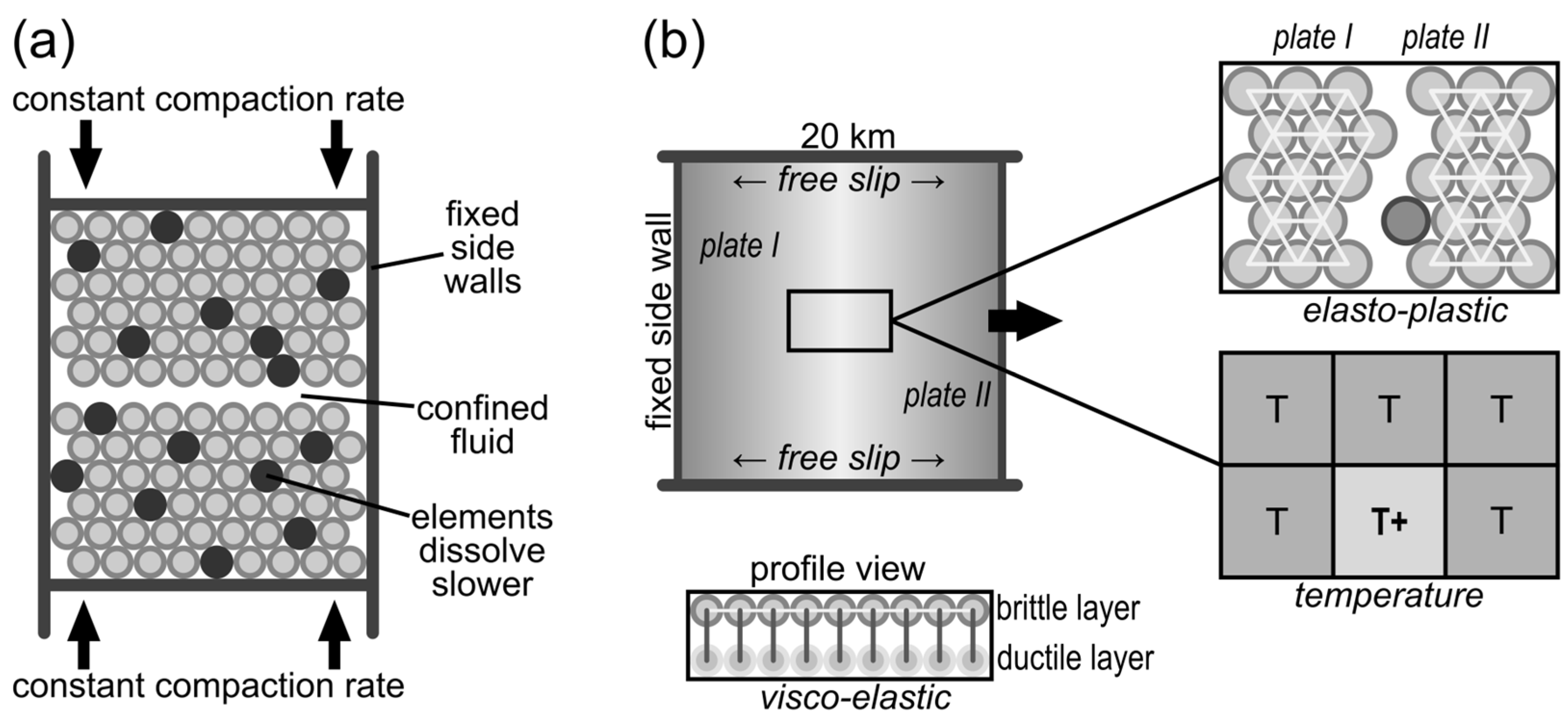
2.1. Numerical Model for Stylolite Simulation

The initial configuration for the stylolite simulation assumes a flat dissolution interface, representing a planar anisotropy in the system (for example, a bedding plane). The boundary conditions involve displacement-controlled movement of the upper and lower walls of the model box, inducing compressive stress at the interface. Elements at the reactive interface dissolve preferentially depending on differences in normal stress, elastic and surface energy. Dissolved elements are removed from the model, and the stress is recalculated to ensure equilibrium.

The dissolution rate (D_i) of each element i is governed by a law derived from thermodynamic principles and a linear kinetic dissolution rate, as follows [8]

$$D_i=k_i{V}_s\left(1-exp{\displaystyle \frac{{-∆\sigma }_n{V}_s-{∆E}_s-{∆E}_{el}}{RT}}\right).$$

(3)

Here, k_i is the dissolution rate constant (mol m⁻² s⁻¹) that can vary between elements, vs. the molecular volume of calcite (m³ mol⁻¹), and Δσ_n is the change in normal stress relative to the average stress at the interface (Pa). ΔE_s and ΔE_el are changes in surface and elastic energies (J m⁻³), respectively, R is the universal gas constant (J mol⁻¹ K⁻¹) and T is the absolute temperature (K). The model assumes that dissolution is the only active process, with dissolved material being instantly distributed, effectively mimicking infinite transport capacity and assuming that the fluid has a concentration of dissolved material that is in equilibrium with the solid being stressed (where we take the average stress along the interface).

Changes in surface energy (ΔE_s) are computed by

$$E_s={\displaystyle \frac{\gamma }{\rho }},$$

(4)

where γ is a constant, the surface free energy (J m⁻²) and ρ is the local radius of curvature (m) of the interface. To determine the local radius of curvature, we used the number of open springs of elements at the dissolution interface and averaged over a number of neighbors [8]. The elastic energy (ΔE_el) is determined by the strain tensor of the spring network:

$$E_{el}={\displaystyle \frac{1}{2}}{\lambda }_1{\left(\sum _i{u}_{ii}\right)}^2+{\lambda }_2\sum _{i,k}{\left(u_{ik}\right)}^2$$

(5)

with λ₁ and λ₂ Lamé constants (Pa), and u_ii and u_ik are derived from the strain tensor of the lattice spring network.

The simulation workflow is as follows [8]:

• Movement application: The system is stressed by incrementally displacing the upper and lower boundaries inward.
• Dissolution calculation: The dissolution rate is evaluated for all elements at the interface, and the element with the highest probability of dissolving is removed.
• Stress redistribution: After element removal, stresses are recalculated to achieve a new equilibrium configuration.
• Iterative Process: Steps 1 to 3 are repeated, progressively roughening the interface.

A certain number of elements can dissolve between the movement steps as a function of a given time step and the time it takes to dissolve the elements.

The model incorporates quenched noise by varying dissolution constants (k_i) among elements to introduce heterogeneity, simulating natural variations in rock properties. For all stylolite simulations, we used parameters identical to those in Koehn et al. [8] and Koehn et al. [4]. The parameters were chosen to reflect the physical properties of calcite (

Table 1. System parameters for stylolite dissolution.

Parameter	Abbreviation	Value	Unit
Molecular volume of calcite	V	4 × 10−5	m3 mol−1
Young’s modulus	E	40	GPa
Poisson’s ratio	λ	0.33	-
Surface free energy	γ	0.27	J m−2
Dissolution rate constant	Di	10−4	mol (m−2 s−1)
Universal gas constant	R	8.3145	J mol−1 K−1
Temperature	T	500	K
Width of the system	-	10	mm
Elements in x-direction	-	50, 100, 200, 400	-

).

We assume that the initial interface starts flat and evolves through dissolution without precipitation. Transport of solutes is assumed to be instantaneous, assuming that diffusion is not rate-limiting. The boundary conditions provide a constant displacement rate, ensuring steady stress application. Absolute time scales are relative due to the simplified dissolution kinetics.

2.2. Numerical Model for MOR and Transform Fault Simulation

In contrast to the stylolite simulations, in the MOR models, no initial anisotropy is inserted. Instead, the model is extended and fractures in the middle. Once the fractures open, new hot elements with a starting temperature of 1200 °C can be inserted, and the ridges start to grow. From that point onwards, the deformation localizes, and the two plates on either side of a new element move away from each other. The new element is randomly added to one of the two plates with equal probabilities. Once a new element is inserted between the plates, the process is repeated, the plates move and the MORs and transform faults develop spontaneously.

The model takes a pseudo-3D approach, with an element layer interconnected by visco-elastic connections that represent the brittle oceanic crust. This layer is coupled to a second visco-elastic layer simulating the ductile behavior of the deeper crust and mantle. Connections in the network can break under stress and heal. New elements can be introduced into the system, representing the emplacement of new hot material. The visco-elastic network is coupled to a temperature field where cooling of the crust is modeled and feeds back to the thermo-mechanical coupling, inducing weakening and healing as a function of temperature.

To simulate the visco-elastic properties, a Maxwell visco-elastic relaxation is used. The evolution of a connection equilibrium length is given by the following:

$${dl}_{t+dt}={dl}_{t}exp\left(-{\displaystyle \frac{G}{\eta }}dt\right),$$

(6)

where G is the shear modulus, η is viscosity and dt is the timestep. As stresses build up, connections may fail due to excessive shear or normal stresses, and these are removed from the network once fractures are open enough so that an element fits into the space, and new elements are introduced, typically at a starting temperature of 1200 °C.

Thermal evolution is computed on a square grid that operates separately from the element arrangement, with each thermal cell twice the width of an element diameter. To avoid artifacts from the two different grid structures, square versus triangular, a tent function [21] interpolates temperature values between the two grids. Cooling is governed by standard thermal diffusion, described by

$${\displaystyle \frac{\partial T}{\partial t}}=\kappa {\displaystyle \frac{{\partial }^{2}T}{\partial x^2}},$$

(7)

where κ is the thermal diffusivity, which is defined as

$$\kappa ={\displaystyle \frac{\lambda }{\rho c}} ,$$

(8)

with the thermal conductivity λ, ρ as the mass density and c as the heat capacity.

In three dimensions, vertical cooling between the base and top of the plate is incorporated. The overall temperature evolution follows an advection–diffusion equation:

$${\displaystyle \frac{\partial \left(T\right)}{\partial t}}+v\nabla \left(T\right)-\kappa \left(∆T-{\displaystyle \frac{T_b-T_a}{4\kappa \left(t-t_i\right)}}\right)=f.$$

(9)

In this equation, v is the plate velocity, T_b and T_a represent the basal and surface temperatures, respectively, and t_i is the time at which an element enters the thermal grid, while t is the current time. The operator ∇ and ∆ refer to the horizontal spatial gradient and Laplacian operators, respectively. Thus, ΔT = ∇ ²T represents the second horizontal spatial derivative of temperature. The source term f is zero except at the MOR axis, where it represents the heat introduced by new elements.

Thermo-mechanical coupling is achieved by allowing material properties such as viscosity, spring constants and breaking strength to vary with temperature. Arrhenius-based relations are used to model these dependencies:

$$\eta =a{{\eta }_0}^{\left({\displaystyle \frac{T_0}{T}}\right)},$$

(10)

$$\ln {\eta }_0={\displaystyle \frac{E_b}{k_B{T}_0}},$$

(11)

where η is the viscosity, a is a weakening factor without dimensions, T is the temperature, T₀ is a reference temperature, E_b is the energy barrier and k_b is the Boltzmann constant. This can also equivalently be written directly in the Arrhenius form:

$$\ln {\eta }_0={\displaystyle \frac{E_b}{k_B{T}_0}}.$$

(12)

Healing is incorporated by introducing new connections that reconnect previously fractured elements. The likelihood of these connections depends on temperature, time and proximity. The healing probability is expressed as

$$P_{heal}=P_0∆t{e}^{-{\displaystyle \frac{E_B}{k_{B}T}}},$$

(13)

where P₀ is the base probability, ∆t is the timestep and E_B is the energy barrier for healing. The energy barrier itself is related to mechanical properties:

$$E_B~Y{\displaystyle \frac{{\left(l_{ij}-d\right)}^2}{d^2}}{V}_p,$$

(14)

where Y is Young’s modulus, l_ij is the distance between elements i and j, d is the element diameter and V_p is the element volume. Substituting into the healing equation, we have the following:

$$P_{heal}=P_0∆t{e}^{-Y{\displaystyle \frac{{\left(l_{ij}-d\right)}^2{V}_p}{ \hspace{0.17em}\hspace{0.17em}{d}^2\hspace{1em}\hspace{0.17em}kT}}}.$$

(15)

Through this integration of mechanical, thermal and healing processes, the model provides a nuanced representation of MOR dynamics. The approach captures key behaviors, including fracture formation, accretion, temperature-driven weakening and the reformation of connections.

The model is divided into two segments: a left-hand side where elements remain stationary and a right-hand side where elements are displaced according to a predefined extension rate. The visco-elastic layer beneath the brittle crust follows the same displacement pattern as the upper layer. After each extension increment, the system is allowed to relax, enabling the redistribution of stress and the development of fractures. Once the system stabilizes at a new equilibrium, the model assesses whether there is sufficient space to introduce new elements into the lattice. If space permits, new elements are added and connected to neighbors within the lattice. This process also allows previously unconnected elements to undergo potential healing, re-establishing connections.

During successive deformation steps, the position of the opening boundary between the two plates progressively shifts toward the right-hand side. This mimics plate divergence, with half of the total extension allocated to each plate. As the MORs evolve, their geometry reflects symmetric growth on both sides of the model. The thermal field is dynamically updated by transferring temperature data between the temperature grid and the solid elements, ensuring that thermal advection accompanies the movement of the plates while also accounting for diffusion.

The model parameters are listed in

Table 2. Model parameters for MOR simulations.

Area of Application	Parameter	Value	Unit
Overall model	Starting Grid Size	200 × 230	Elements
	Real Model Dimension	20 × 20	km
	Real Element Diameter	100	m
	Extension Rate	5	cm year−1
Elastic grid	Young’s Modulus	6–60	GPa
	Breaking Strength	1–10	MPa
Visco-elastic-sheet	Young’s Modulus	6–60	GPa
	Viscosity	1018–1020	Pa s−1
Thermo-mechanical coupling	Healing Probability	0.01	year−1
	kb	1.38 × 10−23	m2 kg s−2 K−1
	Eb	~10−21	m2 kg s−2
	Weakening Factor a	0.2	-
	EB	10−22	m2 kg s−2
Temperature	Grid Space	200	m
	Background Temperature	200	°C
	Inserted Elements (Melt) T	1200	°C
	Ta	20	°C
	Tb	1300	°C
	Thermal Diffusivity κ	~10−6	m2 s−1
	Heat Diffusion Coefficient	10−6	m2 s−1

, providing an overview of the physical dimensions, material properties and thermal conditions used in the simulations. Key values include an element diameter of 100 m, extension rates are 5 cm/year and Young’s modulus values for the brittle crust varying between 6 and 60 GPa. The initial grid size comprises 200 × 230 elements, translating to a real-world domain size of 20 × 20 km.

The pseudo-3D nature of the model reflects a simplification of the complex three-dimensional geometries present in natural MOR systems. The model consists of two primary layers: a visco-elasto-plastic upper crust and a visco-elastic lower layer. While this layered setup effectively captures fracture dynamics, thermal coupling and material weakening, it does not fully account for vertical geometries, such as variations in crustal thickness or topographic relief across transform faults. A key limitation is the inability to model the height differences observed in natural oceanic plates away from MORs and across transform faults. However, the model successfully reproduces critical processes such as MOR propagation, accretion, fault evolution and transform fault development.

The discrete representation of the brittle crust uses constant-sized elements organized initially in a triangular lattice. This arrangement ensures isotropic elastic behavior and stabilizes the insertion of new elements into fractures. Although this triangular grid is altered as fractures develop, the uniform element size prevents significant artifacts. The initial lattice orientation does not appear to influence model results substantially, as the addition of noise to connection-breaking thresholds minimizes grid direction biases. Furthermore, the MOR directions do not align with lattice orientations, and the growing plates lose their grid alignment over time. Therefore, the discrete setup adequately simulates MOR and fault dynamics without introducing significant directional biases.

2.3. Scaling of Dynamic Systems

Dynamic scaling of natural systems includes roughening of interfaces and follows a Family–Vicsek scaling law [1,2,3]. The amplitude of the roughening surface (w(l,t)) as a function of length (l) and time (t) obeys the following scaling law [2,22]:

$$w\left(l,t\right)~l^{H}f\left({\displaystyle \frac{l}{\chi }}\right),$$

(16)

with l being the length of the studied interface, H being the roughness exponent (Hurst exponent) and χ being the correlation length. The universal scaling function f(u) with u = l/χ has the following behavior: if u << 1, then f(u) = const, if u >> 1, then f(u) = u^−H. If the size l of the window that is used to look at the studied interface is smaller than the correlation length χ, the surface has the following behavior [2]:

$$w\left(l,t\right)~l^H.$$

(17)

In this case, the roughening follows a power law of the chosen window size, independent of time, as a function of the roughness exponent. However, if the window is larger than the correlation length, the roughness becomes constant according to [2]

$$w\left(l,t\right)~l^H{\left({\displaystyle \frac{l}{\chi }}\right)}^{-H}={\chi }^H=t^{{\displaystyle \frac{H}{z}}}.$$

(18)

Here, z is the so-called dynamic exponent. The correlation length will grow as a function of time, which in turn leads to an increase in the roughness. Two factors will influence the roughness growth with time, in addition to the roughness exponent: the age of the system and a potential restriction in system size. In terms of age, this means that young stylolites and MORs will be potentially less rough on the large wavelength/amplitude spectrum than older structures. In terms of the system size, for MORs, this could be the size of the ocean or eventually the circumference of the planet. For stylolites, the system size could be a lateral restriction due to layering or other obstacles.

In order to study the scaling properties of these dynamic systems in space and time, we extract a 2-dimensional line from either natural stylolite and MORs or from simulations representing the roughening interface. In the case of stylolites, this line represents the active dissolution interface and, in the case of MORs, it represents the opening MOR segments and associated transform faults. Every point along the length of the structure (x-direction) then has exactly one corresponding point in height (z). We use the term height here for the coordinate perpendicular to the main interface direction, without any reference to the direction of gravity. For the time signal, which can only be studied for simulations, the mean width w_(l) of the interface is calculated for each time step:

$$w_{\left(l\right)}=\sqrt{{\displaystyle \frac{1}{l}}\sum _{i=1}^l{\left[h_i-\overline{h}\right]}^2,}$$

(19)

with h_i (m) as the height at point i on the interface and $\overline{h}$ (m) as the average height of the interface. If the average width of the interface is plotted as a function of time in a log–log plot, the interface width grows with a certain growth exponent until it reaches a correlation length where the width stays constant.

For the space signal, only one time step is needed, so that this scaling can be explored for both numerical and real systems. A height–height correlation function (C(l)) can be used, where the average height is calculated for two points with a given distance l between them:

$$C(l)\equiv \sqrt{\left[{\left(h\left(x\right)-h\left(x^{\prime }\right)\right)}^2\right]}$$

(20)

with h being the height of point x on the interface and l being the distance between point x and x’. If the correlation length is then plotted against the length l in a log–log plot, the systems typically follow a self-affine space series with a roughness exponent until they reach the correlation length, where C(l) becomes constant.

Figure 3 shows the scaling regimes that are typically found for stylolites, with two self-affine scaling regimes in space and time and the third regime where the width is constant. In time, the exponent is termed the growth exponent, and, in space, it is termed the roughness exponent. In stylolites the system goes through a switch between a surface energy dominated regime (I) with growth exponent of 0.5 and a roughness exponent of 1.0 to an elastic energy dominated regime (II) with a growth exponent of about 0.8 and a roughness exponent of 0.5 before reaching the correlation length (regime III) [2,3,4].

3. Results

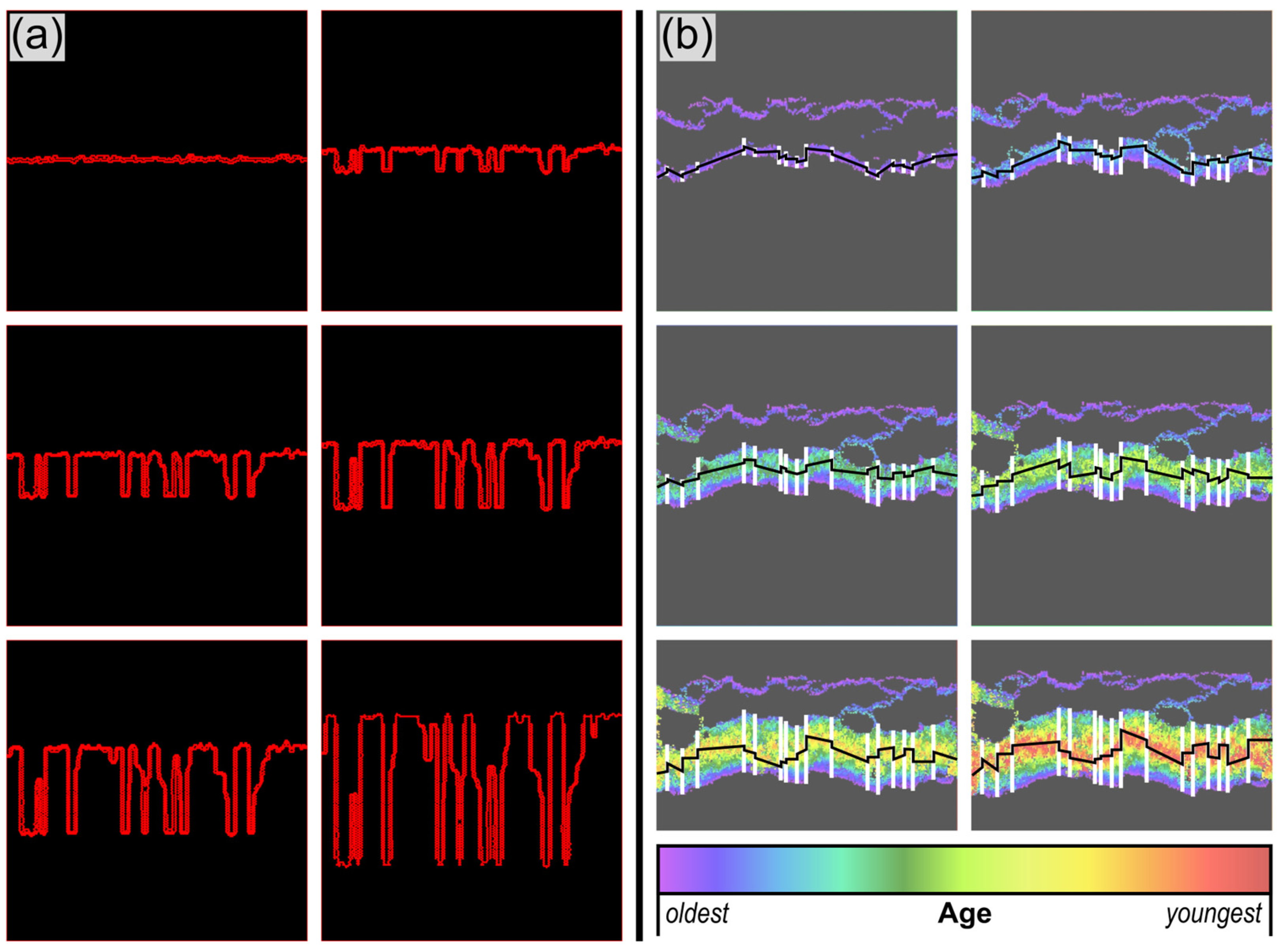
3.1. Simulations of Orthogonal Structures in Stylolites and Ridges

Here, we show simulations of stylolite and MOR development and compare the simulations with natural examples. The evolution of a stylolite and a MOR simulation is shown in Figure 4a,b, where we term both MOR transform faults and the sides of stylolite teeth as “kinematic faults” (KFs). We define “kinematic faults” as faults that develop due to relative movement instead of stress. The stylolite simulation starts from a flat interface (given by the model) within a slowly dissolving layer with an initial roughening [10] that represents the background heterogeneity. Once the layer is breached, the interface moves up or down relative to its initial position as a function of layer pinning on either side. This leads to the growth of relatively long stylolite teeth with KFs that are oriented perpendicular to the initial interface. The spacing of KFs is random and depends on the initial noise, i.e., where the initial layer is breached. Once the layer itself is completely dissolved, the teeth can be destroyed again, leading to a decrease and potential destruction of KFs. The MOR evolution starts at an initially developing fracture (or set of fractures) that develops a long-range wavelength from the beginning. Therefore, the MOR has an initial shape that is different from the relatively straight stylolite (Figure 4a). However, with the progressive opening of the MOR, KFs evolve on top of the initial wavelength. The KFs in the MOR simulation are more active than those in the stylolite simulation in the sense that they are more variable, and KFs in the MOR grow and disappear again. The stylolite has very stable KFs because of its growth from an initial layer, whereas the MOR does not have a layer that stabilizes the interface and leads to fast KF growth. Nonetheless, the KFs are similar in both cases; they develop perpendicular to the interface, show a random spacing and evolve with time, showing an overall roughness growth of the structures.

In contrast to the stylolite shown in Figure 4a, Figure 5a shows a different stylolite simulation [10,20] where the noise is induced by single elements and larger grains. In this case, the interface is more dynamic with stronger fluctuations, where the noise is only present in the background elements, whereas the larger pinning grains produce larger KFs. Figure 5a also shows a comparison between the simulations and natural examples. In the case of stylolites, the natural example also shows pinning on two different noise levels, so that background fluctuations and small-scale roughening can be seen in addition to larger roughening and KF development. The MORs are more complicated interfaces because they are growth structures, so the interface is not always as sharp as it is for the stylolites. The simulated MOR shows clear KFs with variable offset and spacing. In addition, the MORs are partly curving or fluctuating on a small scale in the simulations. The same features are seen in the real example from the South Atlantic. KFs have variable spacing and offsets, and the MORs are not all straight but wavy like those of the simulations. Even though the stylolites develop because of a compression induced by the largest principal stress and the MORs by an extension indicated by the least principal stress, the developing structures are very similar. Both structures show fluctuations and roughness growth, and the development of KFs that are oriented perpendicular to the initial interface. Because both sides of the stylolite interface are pressed together, the KFs show an offset that is in accordance with an offset of the dissolution interface. In contrast, KFs in MORs, because they are extensional with both plates moving away from each other, show an offset at the transforms with the opposite movement.

Another important difference between KFs of stylolites and MORs can be seen in the natural examples in Figure 5. The simulations are all 2D, but in reality, a KF in a stylolite is a tooth, that is, a circular structure in three dimensions with stripes or slicken lines on its sides. In contrast, the MORs are created by plates moving apart from each other with a free surface on the top and the mantle below. In this case, KFs are straight planes, and the height of the oceanic plates varies as a function of plate age.

3.2. Scaling Analysis

In order to compare roughening in stylolites with that of MORs and to understand the associated development of KFs, we treat them as dynamic systems and study their scaling in space, comparing natural examples with simulations (Figure 6). Scaling laws that apply to self-affine systems like stylolites [3,4,20] can also be applied to mid-ocean ridges (Figure 6). In both cases, the active growth or dissolution interface is transferred to a single line, including MOR or stylolite and KFs.

Figure 6 shows the results for stylolites and MOR-KF systems (both simulated and real). First of all, the MOR-KF systems show self-affine scaling properties that are similar to those of stylolites. All systems start with a higher roughness exponent of around 0.7 up to a cross-over where the roughness exponent changes to about 0.3. At the largest scale, the signal becomes flat either as a function of the system size or because the correlation length is reached. The scaling analysis reveals that while KF spacing follows a self-affine distribution, it changes across scales. This can be observed in the simulations as well as the real example from the Atlantic MOR and the real stylolite sample. This means that KFs in stylolites as well as in MOR systems have no dominant spacing but are fractal. The amplitude-to-wavelength ratio changes at a cross-over length scale. On the small scale, the roughness exponent is larger, representing a line that becomes flat very fast. The position of the cross-over scale varies between MOR and stylolites, as well as between simulation and natural examples. For the natural and simulated stylolites, it sits at the millimeter scale, whereas for the real MOR, it is positioned between 200 km and 300 km, and for the modeled MORs on the km scale.

4. Discussion

4.1. Self-Affine Scaling of MORs and Stylolites

Our study on both natural and simulated stylolites and MORs shows that they exhibit self-affine scaling behavior. Scaling analysis on both systems, stylolites and MORs show three regimes: (I) a self-affine scaling regime on the small scale with a roughness exponent between 0.66 and 0.75, (II) an intermediate self-affine regime characterized by a lower roughness exponent of 0.29 to 0.52 and (III) a final regime where the signal goes flat so that the amplitude to wavelength ratio becomes constant [4].

Different self-affine scaling regimes can emerge due to the dominance of different physical processes at different scales. In stylolites, the first regime is controlled by surface energy effects, which lead to a high roughness exponent [3]. In the second regime, elastic energy effects dominate, lowering the roughness exponent. The transition between the two regimes (cross-over length) is a function of the stress on the stylolite and can be used for stress inversion studies [7,24,25,26]. For the simulated and natural stylolite shown in Figure 7a (Yield Cap: stylolites), the cross-over length between the two regimes lies in the millimeters. The third regime shows the end of self-affine scaling when the correlation length is reached. The signal’s amplitude to wavelength ratio becomes constant [4].

The MOR model also exhibits three scaling regimes, with two showing self-affine scaling with similar roughness exponents to the stylolites. However, for the MOR system, even though the roughness exponents are similar, the simulated and natural MOR show very different cross-over points between the scales (300 km for the natural Mid-Atlantic Ridge versus 0.5 km for the simulated MOR; Figure 6c–f). The reason behind this difference in scale transition between simulated and natural MORs could be the fact that the simulation is modeled on a much smaller scale, with only very minor accretion in comparison to the real example. In addition, the simulation may still miss large-scale effects of real MORs. Further, it is also not clear what physical processes are behind the roughness exponents for MORs. At least in the simulation, the smaller scale may be dominated by temperature diffusion acting as short-range interactions, whereas the larger scale may be dominated by elastic effects representing long-range interactions. In real MOR systems, mantle processes may also play a role.

Crucial requirements of both MOR and stylolite roughness growth are initial heterogeneities or noise to initiate the roughening. Noise in stylolite systems is induced by small-scale irregularities, grains, layers and fossils that affect the dissolution [3,20,27,28,29]. The heterogeneities in MORs may result from variations in faulting, varying thermal diffusion, magma supply variations and accretional asymmetries. Opposed to the roughening are stabilizing forces that try to flatten the interface. These forces would be the processes discussed above, as a surface energy domination for stylolites and potentially thermal diffusion for MORs on the small scale and elastic energy for both systems on the large scale. For MORs, there may be more processes involved. For example, Schierjott et al. [30] demonstrated that grain size reduction functions as a driver in transform fault formation and stabilization. Mantle convection can influence MOR segmentation, but it is not universally dominant. The exact role of mantle convection remains uncertain due to our 2.5-dimensional model, where this could not be included. Research by Langemeyer et al. [31] and Ito and Dunn [32] suggests that mantle convection as a large-scale dynamic system may influence divergent plate boundaries. This may be the reason for the real MOR showing scale transition at the 200 to 300 km scale, a length scale that is used as a characteristic distance between transform faults. Our results show that it is not that simple; MORs are self-affine and, as such, do not have a characteristic distance between their transform faults.

These findings support our idea that self-affine roughening is a fundamental characteristic of geological interfaces, governed by competing mechanisms. While the controlling factors vary between MORs and stylolites, the overall scaling behavior is comparable.

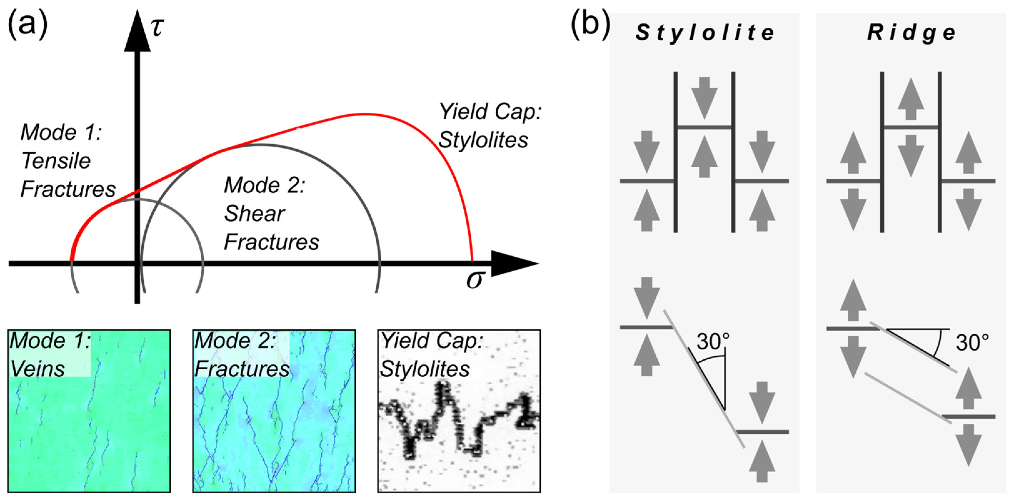
4.2. Kinematic Faults and Their Stability

MORs and stylolites both develop faults and related offsets that are oriented perpendicular to their main roughening interface and are thus oriented parallel to one of the principal stress directions [3,17]. As such, these faults do not contain shear stresses, but are purely developing because of relative movements (Figure 7) or stresses rotate locally around the fault to produce shear stresses. Therefore, they can be understood as kinematic faults (KFs) rather than stress-induced faults, at least on a larger scale. Fault plane solutions show that local stresses around transform faults are producing strike-slip earthquakes, indicating that stresses rotate locally around the faults [33]. In terms of MORs, the transform faults are known to be KFs that are oriented parallel to small circles of plate reconstruction. However, in our model, they also develop without the rotation component and the curvature of Earth’s surface, only as a function of variations in accretion. In stylolites, KFs or the sides of stylolite teeth form due to differences in stress-induced dissolution. As such, they are three-dimensional columns and not straight surfaces like transform faults. Another difference between KFs in stylolites versus MORs is the fact that KFs in MORs merge into fracture zones that can be followed across the ocean floor, which is not the case for stylolites, where KFs are restricted to the dissolution interface. This difference develops because MORs are growth structures in contrast to the dissolving stylolites.

Stylolite teeth and MOR transform faults remain relatively stable once they are established [9]. The MOR-transform fault system can only be destroyed if asymmetric accretion in the ridges leads to their decay or if the ridge jumps to another location [34,35]. They remain stable and active as long as the spreading rate and the ridge position remain stable [36]. Stylolite teeth sides are also relatively stable KFs. They can only be destroyed by differential dissolution or in a similar way to MOR systems with a jump of the stylolite dissolution interface.

Faults in MORs and stylolites that form according to Mohr–Coulomb (Figure 7) would have different orientations in both systems. In stylolites, they would be relatively steeply oriented at an angle of around 60° to the interface. These stress-induced structures could develop into stylolite teeth by rotating slightly. In MORs, stress-induced faults would have an angle of 30° to the interface and, as such, would have an orientation that is not far off that of the ridge itself. These orientations can be found in overlapping ridges.

5. Conclusions

In this contribution, we argue that dissolution and roughening of stylolites at the mineral scale and the development of their teeth can be compared to accretion in MORs and the associated development of transform faults at the tectonic plate scale. We present a new thermos-mechanical model to simulate MORs, where the nucleation and growth of transform faults happen automatically and evolve with time. This can be compared to the roughening growth of stylolites, where teeth evolve and grow during the process. We study and compare the scaling properties of both natural and numerical examples across scales. Our research leads to the following conclusions:

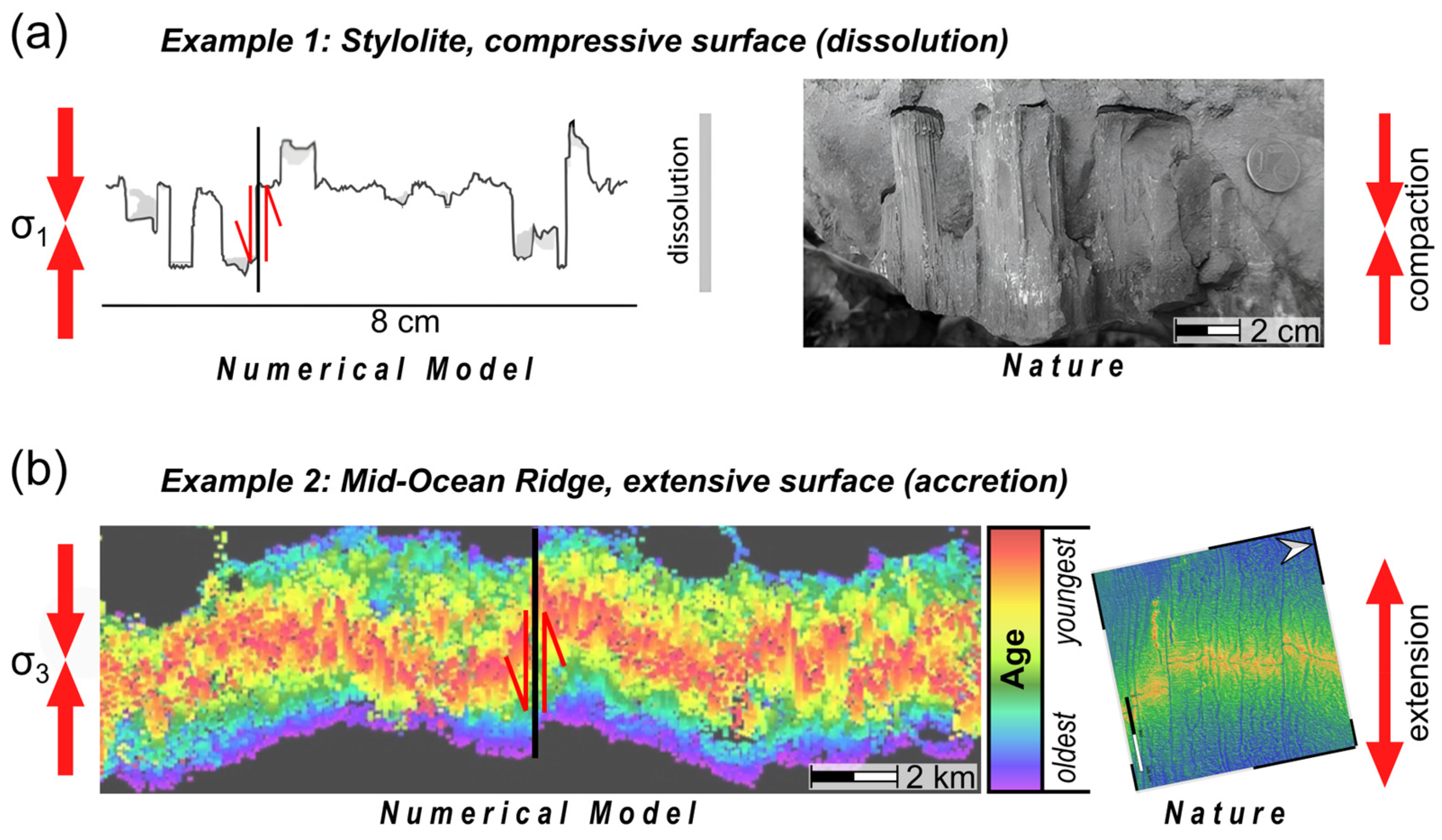
• The development of transform faults in MORs can be seen as part of a dynamic roughening process, much like the stylolite growth at the mineral scale.
• Transform faults and sides of stylolite teeth are similar and represent kinematic faults. These faults do not contain shear stresses and do not follow the Mohr–Coulomb theory since they are not created as a function of stress but as a function of relative movement.
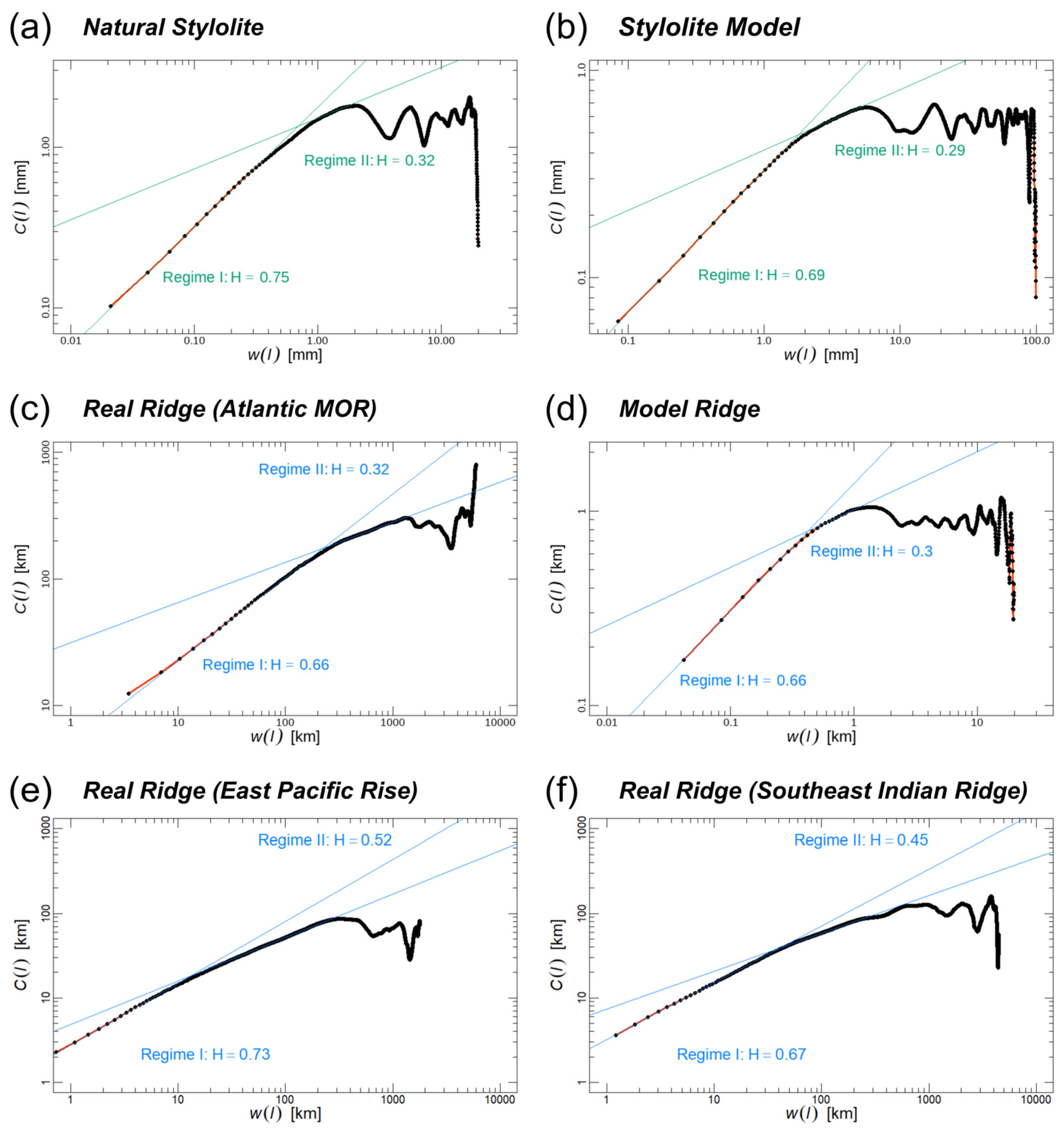
• MORs and stylolites exhibit self-affine scaling properties. This means that the spacing between oceanic transforms associated with MORs does not have a characteristic spacing, but a fractal, much like the fractal scaling of stylolite roughness. The South Atlantic MOR shows a scale transition around 200 to 300 km.
• Simulated and natural MORs and stylolites show two self-affine scaling regimes with different roughness exponents, a higher exponent at smaller scales that transitions to a lower exponent at larger scales. These different regimes should represent the dominance of physical processes at different scales (which are well known for stylolites).

References

1. Barabási, A.-L.; Stanley, H.E. Fractal Concepts in Surface Growth; Cambridge University Press: Cambridge, UK, 2009; ISBN 9780511599798. [Google Scholar]
2. Laronne Ben-Itzhak, L.; Aharonov, E.; Toussaint, R.; Sagy, A. Upper bound on stylolite roughness as indicator for amount of dissolution. Earth Planet. Sci. Lett. 2012, 337–338, 186–196. [Google Scholar] [CrossRef]
3. Toussaint, R.; Aharonov, E.; Koehn, D.; Gratier, J.-P.; Ebner, M.; Baud, P.; Rolland, A.; Renard, F. Stylolites: A review. J. Struct. Geol. 2018, 114, 163–195. [Google Scholar] [CrossRef]
4. Koehn, D.; Koehler, S.; Toussaint, R.; Ghani, I.; Stollhofen, H. Scaling analysis, correlation length and compaction estimates of natural and simulated stylolites. J. Struct. Geol. 2022, 161, 104670. [Google Scholar] [CrossRef]
5. Power, W.L.; Tullis, T.E. Euclidean and fractal models for the description of rock surface roughness. JGR Solid Earth 1991, 96, 415–424. [Google Scholar] [CrossRef]
6. Renard, F.; Schmittbuhl, J.; Gratier, J.-P.; Meakin, P.; Merino, E. Three-dimensional roughness of stylolites in limestones. JGR Solid Earth 2004, 109, B3. [Google Scholar] [CrossRef]
7. Schmittbuhl, J.; Renard, F.; Gratier, J.P.; Toussaint, R. Roughness of stylolites: Implications of 3D high resolution topography measurements. Phys. Rev. Lett. 2004, 93, 238501. [Google Scholar] [CrossRef] [PubMed]
8. Koehn, D.; Renard, F.; Toussaint, R.; Passchier, C.W. Growth of stylolite teeth patterns depending on normal stress and finite compaction. Earth Planet. Sci. Lett. 2007, 257, 582–595. [Google Scholar] [CrossRef]
9. Aharonov, E.; Katsman, R. Interaction between pressure solution and clays in stylolite development: Insights from modeling. Am. J. Sci. 2009, 309, 607–632. [Google Scholar] [CrossRef]
10. Koehn, D.; Rood, M.P.; Beaudoin, N.; Chung, P.; Bons, P.D.; Gomez-Rivas, E. A new stylolite classification scheme to estimate compaction and local permeability variations. Sediment. Geol. 2016, 346, 60–71. [Google Scholar] [CrossRef]
11. Olive, J.-A.; Dublanchet, P. Controls on the magmatic fraction of extension at mid-ocean ridges. Earth Planet. Sci. Lett. 2020, 549, 116541. [Google Scholar] [CrossRef]
12. Zhou, D.; Li, C.-F.; Zlotnik, S.; Wang, J. Correlations between oceanic crustal thickness, melt volume, and spreading rate from global gravity observation. Mar. Geophys. Res. 2020, 41, 14. [Google Scholar] [CrossRef]
13. Morgan, J.P.; Chen, Y.J. The genesis of oceanic crust: Magma injection, hydrothermal circulation, and crustal flow. JGR Solid Earth 1993, 98, 6283–6297. [Google Scholar] [CrossRef]
14. Sempéré, J.-C.; Lin, J.; Brown, H.S.; Schouten, H.; Purdy, G.M. Segmentation and morphotectonic variations along a slow-spreading center: The Mid-Atlantic Ridge (24°00′ N–30°40′ N). Mar. Geophys. Res. 1993, 15, 153–200. [Google Scholar] [CrossRef]
15. Choi, E.; Lavier, L.; Gurnis, M. Thermomechanics of mid-ocean ridge segmentation. Phys. Earth Planet. Inter. 2008, 171, 374–386. [Google Scholar] [CrossRef]
16. Wilson, J.T. A New Class of Faults and their Bearing on Continental Drift. Nature 1965, 207, 343–347. [Google Scholar] [CrossRef]
17. Gerya, T. Origin and models of oceanic transform faults. Tectonophysics 2012, 522–523, 34–54. [Google Scholar] [CrossRef]
18. Murton, B.J.; Rona, P.A. Carlsberg Ridge and Mid-Atlantic Ridge: Comparison of slow spreading centre analogues. Deep. Sea Res. Part II Top. Stud. Oceanogr. 2015, 121, 71–84. [Google Scholar] [CrossRef]
19. Bons, P.D.D.; Koehn, D.; Jessell, M.W. Microdynamics Simulation; Springer: Berlin/Heidelberg, Germany, 2008; ISBN 9783540447931. [Google Scholar]
20. Koehn, D.; Ebner, M.; Renard, F.; Toussaint, R.; Passchier, C.W. Modelling of stylolite geometries and stress scaling. Earth Planet. Sci. Lett. 2012, 341–344, 104–113. [Google Scholar] [CrossRef]
21. Ghani, I.; Koehn, D.; Toussaint, R.; Passchier, C.W. Dynamic Development of Hydrofracture. Pure Appl. Geophys. 2013, 170, 1685–1703. [Google Scholar] [CrossRef]
22. Family, F.; Vicsek, T. Scaling of the active zone in the Eden process on percolation networks and the ballistic deposition model. J. Phys. A Math. Gen. 1985, 18, L75–L81. [Google Scholar] [CrossRef]
23. Ebner, M.; Toussaint, R.; Schmittbuhl, J.; Koehn, D.; Bons, P. Anisotropic scaling of tectonic stylolites: A fossilized signature of the stress field? JGR Solid Earth 2010, 115, B6. [Google Scholar] [CrossRef]
24. Köhler, S.; Duschl, F.; Fazlikhani, H.; Koehn, D.; Stephan, T.; Stollhofen, H. Reconstruction of cyclic Mesozoic–Cenozoic stress development in SE Germany using fault-slip and stylolite inversion. Geol. Mag. 2022, 159, 2323–2345. [Google Scholar] [CrossRef]
25. Beaudoin, N.; Lacombe, O.; Koehn, D.; David, M.-E.; Farrell, N.; Healy, D. Vertical stress history and paleoburial in foreland basins unravelled by stylolite roughness paleopiezometry: Insights from bedding-parallel stylolites in the Bighorn Basin, Wyoming, USA. J. Struct. Geol. 2020, 136, 104061. [Google Scholar] [CrossRef]
26. Beaudoin, N.; Lacombe, O. Recent and future trends in paleopiezometry in the diagenetic domain: Insights into the tectonic paleostress and burial depth history of fold-and-thrust belts and sedimentary basins. J. Struct. Geol. 2018, 114, 357–365. [Google Scholar] [CrossRef]
27. Ebner, M.; Piazolo, S.; Renard, F.; Koehn, D. Stylolite interfaces and surrounding matrix material: Nature and role of heterogeneities in roughness and microstructural development. J. Struct. Geol. 2010, 32, 1070–1084. [Google Scholar] [CrossRef]
28. Rustichelli, A.; Tondi, E.; Agosta, F.; Cilona, A.; Giorgioni, M. Development and distribution of bed-parallel compaction bands and pressure solution seams in carbonates (Bolognano Formation, Majella Mountain, Italy). J. Struct. Geol. 2012, 37, 181–199. [Google Scholar] [CrossRef]
29. Rustichelli, A.; Tondi, E.; Korneva, I.; Baud, P.; Vinciguerra, S.; Agosta, F.; Reuschlé, T. Bedding-parallel stylolites in shallow-water limestone successions of the Apulian Carbonate Platform (central-southern Italy). Ital. J. Geosci. 2015, 134, 513–534. [Google Scholar] [CrossRef]
30. Schierjott, J.C.; Thielmann, M.; Rozel, A.B.; Golabek, G.J.; Gerya, T.V. Can Grain Size Reduction Initiate Transform Faults?—Insights From a 3-D Numerical Study. Tectonics 2020, 39, 10. [Google Scholar] [CrossRef]
31. Langemeyer, S.M.; Lowman, J.P.; Tackley, P.J. Global mantle convection models produce transform offsets along divergent plate boundaries. Commun. Earth Environ. 2021, 2, 69. [Google Scholar] [CrossRef]
32. Ito, G.; Dunn, R.A. Mid-Ocean Ridges: Mantle Convection and Formation of the Lithosphere. In Encyclopedia of Ocean Sciences; Elsevier: Amsterdam, The Netherlands, 2009; pp. 867–880. ISBN 9780123744739. [Google Scholar]
33. Abercrombie, R.E.; Ekström, G. Earthquake slip on oceanic transform faults. Nature 2001, 410, 74–77. [Google Scholar] [CrossRef] [PubMed]
34. Mittelstaedt, E.; Ito, G.; Behn, M.D. Mid-ocean ridge jumps associated with hotspot magmatism. Earth Planet. Sci. Lett. 2008, 266, 256–270. [Google Scholar] [CrossRef]
35. Wei, J.; Dai, S.; Cheng, H.; Wang, H.; Wang, P.; Li, F.; Xie, Z.; Zhu, R. Review of Asymmetric Seafloor Spreading and Oceanic Ridge Jumps in the South China Sea. J. Mar. Sci. Eng. 2024, 12, 408. [Google Scholar] [CrossRef]
36. Harper, H.; Luttrell, K.; Sandwell, D.T. Ridge Propagation and the Stability of Small Mid-Ocean Ridge Offsets. J. Geophys. Res. Solid Earth 2023, 128, 8. [Google Scholar] [CrossRef]
Figure 1. Comparison of (a) sedimentary stylolite with pronounced teeth from the German Zechstein Carbonates [10]. The width of the view is 1 cm. These pronounced rectangular stylolites are thought to develop on sedimentary layers. (b) Mid-ocean ridge (MOR) in the South Atlantic with pronounced transform faults. Note that the spacing of the transform faults is not regular. In addition, they have a similarity with stylolite teeth.
Minerals 15 00743 g001
Figure 2. (a) Schematic setup for stylolite modeling. Two rocks represented by elastic elements that can dissolve are pressed together at an interface. The elements will then dissolve as a function of differences in stress, elastic and surface energy. The noise in the system is set by different dissolution constants of single elements, large grains (made up of multiple elements) and layers [8]. (b) Setup for MOR modeling where two plates are pulled apart from each other. Once a fracture opens, new hot elements are introduced to model accretion. Heat diffusion is calculated in a second grid and in pseudo-third dimension, the plate model is attached to a viscous “mantle” layer.
Minerals 15 00743 g002
Figure 3. Stylolite scaling in self-affine time and space series (after Koehn et al. [4]). (a) Time series with three scaling regimes, two self-affine regimes (I and II) with growth exponents β and a third regime (III), where the stylolite width becomes constant. (b) Space series with the same three scaling regimes (self-affine regimes I and II and a constant regime III). The regimes are characterized by their roughness exponent α [1,2,3,8,23].
Minerals 15 00743 g003
Figure 4. Simulation of (a) stylolite development from an initial layer and (b) MOR development from an initial fracture. Progressive evolution shows the development of kinematic faults (KFs) in both cases, even though the development of the stylolite KFs is more extreme because of the initially pinning layer. The MOR model starts out rougher because it follows initial fractures, but then starts to develop KFs that grow with time. White vertical lines mark KFs, the black fluctuating line follows the spreading center.
Minerals 15 00743 g004
Figure 5. Comparison of (a) a stylolite simulation with a real stylolite in example 1. In this case, the stylolite simulation is initiated by background noise and larger grains that pin the interface in contrast to a layer, as in Figure 4a. Because the stylolites show dissolution, the interface is clearly visible as a dark line that collects insoluble material in the real case. And (b) a MOR simulation with a real ridge in example 2. It shows a MOR simulation that started at a fracture and that develops vertical KFs similar to the natural example on the right-hand side of the North Atlantic MOR. The interface is more complicated in the MOR simulation because it is a growth feature, with the color scale in the simulation indicating different ages of elements (from purple (old) to red (young)). In the real example, a height map illustrates the different ages with the young parts in yellow and the old parts in blue.
Minerals 15 00743 g005
Figure 6. Correlation functions of (a) a natural stylolite (from the Kirchleus quarry in Northern Bavaria [4]), (b) a modeled stylolite (from Figure 5a [10]), (c) a natural MOR (southern part of the mid-Atlantic ridge), (d) a simulated MOR-KF system, (e) a natural MOR (East Pacific Rise) and (f) a natural MOR (Southwest Indian Ridge). Greenish colors in (a,b) are used for stylolites, bluish colors in (cf) are used for MORs.
Minerals 15 00743 g006
Figure 7. (a) Mohr–Coulomb circle. Mode 1 (tensile fractures) covers tectonic features like veins, Mode 2 (shear fractures) results in fractures, while stylolites are the result of stress beyond the Yield Cap. (b) Stress directions (arrows) in stylolites and MOR environment force their tectonic features to stress equilibria.
Minerals 15 00743 g007