Automated Hyperspectral Ore–Waste Discrimination for a Gold Mine: Comparative Study of Data-Driven and Knowledge-Based Approaches in Laboratory and Field Environments

Abstract

Hyperspectral imaging has been increasingly used in mining for detailed mineral characterization and enhanced ore–waste discrimination, which is essential for optimizing resource extraction. However, the full deployment of this technology still faces challenges due to the variability of field conditions and the spectral complexity inherent in real-world mining environments. In this study, we compare the performance of two approaches for ore–waste discrimination in both laboratory and actual mine site conditions: (i) a data-driven feature extraction (FE) method and (ii) a knowledge-based mineral mapping method. Rock samples, including ore and waste from an open-pit gold mine, were obtained and scanned using a hyperspectral imaging system under laboratory conditions. The FE method, which quantifies the frequency absorption peaks at different wavelengths for a given rock sample, was used to train three discriminative models using the random forest classifier (RFC), support vector classification (SVC), and K-nearest neighbor classifier (KNNC) algorithms, with RFC achieving the highest performance with an F1-score of 0.95 for the laboratory data. The mineral mapping method, which quantifies the presence of pyrite, calcite, and potassium feldspar based on prior geochemical analysis, yielded an F1-score of 0.78 for the ore class using the RFC algorithm. In the next step, the performance of the developed discriminative models was tested using hyperspectral data of two muck piles scanned in the open-pit gold mine. The results demonstrated the robustness of the mineral mapping method under field conditions compared to the FE method. These results highlight hyperspectral imaging as a valuable tool for improving ore-sorting efficiency in mining operations.

1. Introduction

Mining operations are characterized by large quantities of extracted material that necessitate efficient discrimination between ore and waste to optimize resource utilization. Accurate and timely discrimination between ore and waste materials is crucial for optimizing the mining and milling process. Precise tagging of the extracted material allows for better control of ore dilution and ore loss, enhancing overall resource management [1,2]. This can reduce the amount of waste fed to the mineral processing plant, reducing the amount of energy in the comminution process per ton of the final product that is produced. In addition, the amount of tailing materials produced at the processing plant can be reduced. In conventional methods, the ore zone in the blasted muck pile is subjectively identified through dig lines by ore-control geologists based on their prior knowledge of the ore body, visual observations, and blast-induced rock movement data [3,4]. The process is time-consuming and inaccurate and can impose hazardous conditions on technical staff when walking on a blasted muck pile. In general, the economic feasibility of a mining operation depends on the ability to extract valuable minerals while minimizing the extraction of waste materials. Thus, advancements in ore–waste discrimination technologies contribute significantly to sustainable and more efficient mining practices.

In recent years, the integration of hyperspectral imaging technology has been demonstrated as a promising solution for automating the ore–waste discrimination process. Hyperspectral sensors capture a broad range of wavelengths, providing detailed spectral information for each pixel in an image. This capability opens up new opportunities for precise mineral identification, improving efficiency and cost-effectiveness in mining operations. The spectral signatures obtained enable the differentiation of minerals based on their unique absorption and reflection patterns, setting the stage for enhanced geological interpretations and resource assessments. Previous studies have demonstrated the efficiency of hyperspectral imaging in various mining applications, emphasizing its ability to enhance geological mapping, mineral exploration, and ore characterization. Numerous researchers have demonstrated the use of hyperspectral imaging for the mapping of minerals, the delineation of ore zones, and the identification of geological structures [5,6,7,8,9,10,11]. In the specific context of ore–waste discrimination, Dalm et al. [12] explored the use of near-infrared and short-wavelength infrared (SWIR) hyperspectral imagery to distinguish between ore and waste particles in epithermal deposits. Through maps generated from hyperspectral images of drill core samples, the researchers applied partial least squares discriminant analysis to identify waste samples. Lypaczewski et al. [13] highlighted the application of hyperspectral imagery in characterizing the Canadian Malartic gold deposit, emphasizing its effectiveness in visualizing mineralogical changes related to metamorphism and hydrothermal alteration. The study demonstrates the correlation between white mica composition and gold content, enabling discrimination between unmineralized, weakly mineralized, and highly mineralized samples. Tuşa et al. [14] introduced a novel approach to assess the efficiency of sensor-based ore sorting using hyperspectral visible to near-infrared (VNIR) and SWIR sensors. Machine-learning classification methods, the support vector classifier (SVC) and random forest classifier (RFC) techniques, were successfully tested on two complex ores: a tin ore with variable cassiterite distribution and a copper–gold porphyry with diverse copper and gold mineral compositions. The results demonstrated promising sorting outcomes, indicating the potential applicability of the approach across various ore types, thereby enhancing the attractiveness of VNIR-SWIR sensors in the sorting of minerals. Abdolmaleki et al. [4] investigated the use of hyperspectral remote sensing and deep learning for discrimination of ore and waste in a Silver deposit using half-core rock samples. By training a deep learning model on hyperspectral images of the core samples, the approach outperformed conventional methods, achieving high overall accuracy. These findings suggest the potential for practical and efficient ore and waste classification in near real-time using integrated hyperspectral imaging and machine-learning techniques. El Mansour et al. [15] explored the application of hyperspectral imaging combined with explainable machine-learning techniques for classifying phosphate mining waste. By integrating convolutional neural networks with the Shapley additive explanations method, they achieved a classification accuracy of 92%, successfully distinguishing between carbonate-rich, phosphate-rich, clay, and siliceous waste types. Their findings highlight the potential of hyperspectral imaging for real-time, sustainable waste management in mining operations. Zhang et al. [16] investigated the quantitative unmixing of mixed mineral components using hyperspectral data, focusing on mixtures of dolomite and gypsum. They proposed three improved spectral decomposition models: the continuum removal-fully constrained linear spectral model, the natural logarithm-fully constrained linear spectral model (NL-FCLSM), and the ratio derivative model. Their results demonstrated that the NL-FCLSM model provided the highest accuracy, significantly reducing abundance error compared to traditional linear unmixing methods. This study highlights the potential of advanced unmixing techniques for improving mineral discrimination in complex geological materials.

Remote-sensing applications commonly leverage diverse data analytics and classification techniques to extract valuable information from spectral data. SVC [17], RFC [18], and KNNC [19] are among the commonly utilized methods for mining-related classification tasks. RFC and SVC stand out as promising algorithms in remote sensing, especially in hyperspectral imaging. Numerous studies have showcased the efficacy of SVC for mineral mapping and geological applications, as evidenced by References [20,21,22,23,24]. Similarly, RFC has been widely employed for mining-related classification tasks in remote sensing, especially in hyperspectral imaging, as demonstrated by References [25,26,27,28,29]. While KNNC may not be as commonly utilized as RF and SVM in the context of geology with hyperspectral data, some research efforts are still being made to explore its application in this field. Several studies, such as those conducted by the researchers in [30,31,32], have investigated the effectiveness of KNNC for geology mapping purposes.

Machine-learning (ML) techniques have shown promise in automating discrimination but often require extensive feature engineering and may struggle with the high-dimensional nature of hyperspectral data. As mining operations become more complex, there is a growing need for innovative approaches that overcome these limitations and provide robust solutions for accurate and efficient discrimination. To address these challenges, two distinct approaches are used for the ore–waste discrimination: data-driven feature extraction (FE) and knowledge-based mineral potential mapping (MPM). MPM is a well-established geological approach that uses prior mineralogical knowledge to explain ore zones. This method is particularly useful in mining because mineralogical variations often correlate with ore grades. By mapping key minerals, MPM provides a geological context for ore–waste discrimination. It has been widely applied in exploration, but its application in real-time ore–waste discrimination has been relatively unexplored. In contrast, data-driven methods, such as hyperspectral imaging combined with machine learning, offer a more automated approach by extracting spectral features from ore and waste materials.

Hyperspectral imaging sensors have gained increasing recognition for their effectiveness in lithological and mineralogical analysis at the laboratory scale, particularly for hand-picked specimens and drill cores [14,33]. When conducting under controlled laboratory settings, i.e., sufficient lighting, fixed sensor-to-sample distances, and stable environmental parameters, hyperspectral data acquisition enables precise spectral characterization and detailed mineral analysis [34]. However, applying these techniques in operational mining environments presents significant challenges due to the spectral variability introduced by environmental factors such as moisture, dust, and inconsistent lighting conditions.

This study presents a novel comparative analysis of knowledge-based mineral mapping and data-driven FE for ore–waste discrimination using hyperspectral imaging in both laboratory and active mine settings. A key innovation lies in the multi-scale application—from hand-picked sample analysis in controlled lab conditions to full-scale muck pile assessments in an operational open-pit gold mine. We compare the performance of classifier models developed using the results of the mineral potential mapping (MPM) approach, which uses the spectral angle mapper (SAM) for expert-guided mineral identification, with classifier models developed based on spectral FE for automated discrimination. By evaluating accuracy, reliability, and adaptability using both laboratory and actual mine site data, we highlight the contrasts between expert-driven geological interpretation and automated spectral classification. This work is distinguished by (1) the direct comparison of two fundamentally different classification strategies, (2) the use of laboratory data for model training and subsequent field application following adjustment for in situ conditions, and (3) performance testing under operational mining conditions, an aspect rarely addressed in prior studies. This dual-method framework, supported by field validation, contributes to advancing the practical use of hyperspectral imaging in mining operations.

In this research, we utilized hyperspectral SWIR data (300 spectral bands from 970 nm to 2500 nm) collected from rock samples and muck piles at an open-pit gold mine for ore–waste discrimination analysis. SWIR data provides a more detailed and informative view of mineral identification and discrimination. Different studies have demonstrated the employment of SWIR data in geological mapping applications [35,36,37].

This research bridges the gap between laboratory-scale hyperspectral analysis and actual mining operations, providing new insights into the adaptability, robustness, and practical feasibility of hyperspectral remote sensing for real-time ore–waste discrimination. These findings support more informed decision-making in mining, contributing to the ongoing transformation toward automated, efficient, and sustainable mineral resource management.

2. Materials and Methods

2.1. Data Collection

The study area is located in an open-pit gold mine in Canada, with an average gold grade of ~1.0 g/t. It represents a world-class example of a large-tonnage, low-grade open-pit gold operation. Geologically, the central part of the deposit is hosted within the metasedimentary rocks of the Pontiac Group and partly within the metavolcanic rocks of the Piché Group. The unaltered metasedimentary rocks consist of interlayered greenish-grey mudstones and brownish-grey greywackes, with individual beds reaching up to several meters in thickness. Common minerals within these rocks include quartz, plagioclase, white mica, biotite, and chlorite.

The deposit is characterized by a continuous shell containing 1% to 5% disseminated pyrite, which is closely associated with fine native gold and minor occurrences of chalcopyrite, sphalerite, and tellurides. Approximately 70% of the gold resource is hosted within the altered clastic sedimentary rocks of the Pontiac Group, which overlie an epizonal dioritic porphyry intrusion. The remaining 30% of the deposit is situated within the upper portions of this porphyry body. Alteration in the sedimentary rocks is dominated by potassic alteration (biotite–sericite–carbonate assemblage), overprinted by pervasive silica and carbonate alteration. The carbonate minerals are primarily calcite, with minor amounts of ankerite.

2.1.1. Laboratory Data Collection

The dataset used comprises 178 hand-picked rock samples sourced from six blasted muck piles within the open-pit mine. The samples are categorized into two primary groups: sediment and ultramafic. The collected samples were scanned using a hyperspectral imaging system at the University of Toronto’s Mine Modeling and Analytics lab. The HySpex Mjolnir VS-620 (Neo, Oslo, Norway) imaging system includes VNIR and SWIR sensors, covering a broad electromagnetic spectrum that spans from 400 to 2500 nm. The process involves scanning the samples while adjusting integration time, using a white target panel to convert radiance to reflectance. The specifications of the sensors used are listed in

Table 1. Main specifications of the HySpex Mjolnir VS-620 imaging system.

	V-1240	S-620
Spectral range	400–1000 nm	970–2500 nm
Spatial pixels	1240	620
Spectral channels and sampling	200 bands @ 3.0 nm	300 bands @ 5.1 nm
F-number	F1.8	F1.9
FOV	20°	20°
Pixel FOV across/along	0.27/0.54 mrad	0.54/0.54 mrad
Bit resolution (raw data)	12 bit	16 bit
Dynamic range	4400	10,000
Max speed (at full resolution)	200 fps	170 fps

.

Figure 1 illustrates the setup employed for scanning the collected samples, comprising the Hyspex VS-620 camera, halogen lamps, white reflectance panels, and the samples. The camera is positioned at a height of 1 m from the rock samples, and two lenses (one for VNIR and one for SWIR) were used for short-distance scanning. The light sources cover the entire range of VNIR and SWIR (400 to 2500 nm). The scanning process involved three distinct white reflectance panels (20%, 50%, and 90% reflectance) at varying tray speeds. After assessing saturation levels in the scanned sample images, it was decided to proceed with a white reflectance of 50% and an average tray speed of 25 mm/s for subsequent analysis.

As strong absorption features of hydrothermal mineralization generally occur in the SWIR region, the VNIR data were excluded from further analysis to avoid complicated processing [38,39]. The absorption features within the SWIR region offer unique insights into the composition of geological materials, with distinctive absorption features arising from the presence of hydroxyl (OH) groups in minerals. In the context of this study, the primary alteration patterns associated with gold mineralization at the study site are hydrothermal in nature, specifically potassic, carbonate, and silica overprinting, which are best captured in the SWIR region via diagnostic OH- and CO₃-related absorptions (e.g., near 1400, 1900, 2200, and 2350 nm) [40]. Given this mineralogical context, our classification framework prioritized minerals such as biotite–sericite–carbonate assemblages, which are more spectrally expressive in SWIR. Furthermore, including VNIR data introduced challenges related to data fusion and model robustness, especially under variable illumination conditions and rock surface textures in field-collected samples. In addition, SWIR sensors typically offer more channels than visible and VNIR sensors, allowing for more detailed and accurate characterization of mineral spectra. For some samples, both sides of the rock were subjected to scanning, resulting in a total of 246 SWIR images.

The scanned rock samples were sent for fire assay and mineralogical analysis at the ALS Geochemistry lab, Sudbury, ON, Canada, to extract additional insights into their composition, including gold assays and mineralogical composition of the rock samples. Based on the mine’s cut-off grade of 0.25 ppm and the fire assay results, all samples were classified as either ore or waste. This classification was essential for the development and training of our discrimination predictive model. A total of 102 hyperspectral images were designated as ore, while 144 images were classified as waste. Regarding mineralogical analysis, selected rock samples from the study area were examined using X-ray diffraction (XRD). The XRD results confirmed the presence of key alteration minerals, including biotite, muscovite, chlorite, albite, pyrite, and quartz, consistent with the observed potassic and carbonate alteration patterns. Notably, higher gold grades were associated with samples showing more intense potassium feldspar alteration and elevated pyrite content, supporting the interpretation that hydrothermal alteration minerals are closely linked to gold mineralization within the deposit. In addition, a positive correlation was observed between calcite abundance and gold assay values. Based on these findings, potassium feldspar, pyrite, and calcite were selected as reference minerals for the mineral potential mapping approach to discriminate ore from waste (

Table 2. The result of XRD analysis on the 34 selected rock samples.

Sample	Q	B	M	Ch	D	Ca	P	T	M	H	A	Po	Au
Pile1-01	13	1	0	0	0	6	3	0	0	0	47	30	0.595
Pile1-05	31	10	5	0	0	3	1	0	0	0	44	6	0.434
Pile1-10	19	16	12	1	0	1	1	0	0	0	38	12	1.215
Pile1-32	28	5	8	2	0	5	1	0	0	0	39	11	1.41
Pile1-48	20	1	2	1	0	7	4	0	0	0	22	43	4.7
Pile2-01	29	10	13	7	0	0	0	0	0	0	35	4	0.069
Pile2-02	31	9	24	5	0	0	0	0	0	0	28	2	0.055
Pile2-04	27	13	15	2	0	1	0	0	0	0	37	4	0.123
Pile2-08	18	16	1	2	0	0	1	0	0	0	55	5	0.274
Pile3-01	19	2	3	6	0	4	2	0	0	0	42	22	2.17
Pile3-02	0	0	0	23	6	7	0	51	3	9	1	0	0.04
Pile3-04	1	17	0	1	0	1	0	4	1	71	0	3	0.003
Pile3-06	0	0	0	24	5	3	0	59	4	3	1	0	0.019
Pile3-09	0	27	0	4	0	3	0	1	0	25	33	3	0.025
Pile3-12	24	2	4	0	0	0	0	0	0	0	64	5	0.0005
Pile4-01	0	0	0	25	8	6	0	43	5	13	1	0	0.024
Pile4-03	0	35	0	2	0	5	0	2	0	7	39	4	0.04
Pile4-04	0	26	0	10	3	4	0	9	3	41	0	3	0.096
Pile4-05	13	3	4	0	0	3	0	0	0	0	72	5	0.201
Pile4-08	23	3	6	0	0	1	0	0	0	0	53	13	0.134
Pile4-10	10	3	3	0	0	3	1	0	0	0	70	8	0.574
Pile5-01	1	33	3	4	33	1	1	23	1	0	0	0	0.018
Pile5-02	30	12	13	3	0	0	0	0	0	0	37	4	0.004
Pile5-03	28	12	3	2	0	0	0	0	0	0	47	5	0.001
Pile5-04	0	1	0	24	10	0	0	11	6	48	0	0	0.005
Pile5-09	4	29	1	2	25	1	1	36	2	0	0	0	0.021
Pile5-10	2	2	0	24	6	1	0	16	5	31	13	0	0.002
Pile5-22	0	0	0	27	7	0	1	33	7	16	0	0	0.003
Pile5-37	0	10	0	8	0	0	0	0	0	76	1	2	0.002
Pile5-42	35	1	18	5	0	3	1	0	0	0	31	5	0.09
Pile6-01	0	5	0	22	8	4	0	48	4	9	1	0	0.006
Pile6-02	0	57	0	19	0	4	0	1	9	0	0	2	0.021
Pile6-08	0	4	0	19	9	5	0	40	3	20	0	0	0.006
Pile6-13	0	6	0	25	0	5	0	3	3	56	0	1	0.004

Q: Quartz, B: Biotite, M: Muscovite, Ch: Chlorite, D: Dolomite, Ca: Calcite, P: Pyrite, T: Talc, M: Magnetite, H: Hornblende, A: Albite, Po: Potassium Feldspar (all in percent), Au: Gold (ppm).

).

2.1.2. Field Data Collection

Two muck piles were scanned in the open-pit mine where rock samples had been previously collected for laboratory-scale analysis. To scan the muck piles, the HySpex Mjolnir VS-620 hyperspectral camera was mounted on a custom-built tripod equipped with a programmable rotation stage designed to enable stable scanning at a consistent speed. The tripod features an adjustable height of up to 2 m, and the camera can be tilted to capture the upper portions of the pile. Due to the technical limitations of the VS-620, the maximum achievable rotation speed is 3.1 rad/s. It is important to note that scanning speed directly affects the amount of energy received by the sensor for each scan line, with higher rotation speeds resulting in lower energy capture. The optimum rotation speed is influenced by several factors, including the albedo of the rocks, the horizontal distance between the camera and the pile, and ambient lighting conditions. Through experience gained from various scanning sessions, the optimal rotation speed for each pile was determined to be between 1 and 3 rad/s. The scanning of the muck piles was conducted with the same hyperspectral camera, positioned approximately 20 m from the piles. A (50 cm × 50 cm) Spectralon 50% white reflectance standard panel was placed near the piles to calibrate the recorded data and convert radiance measurements into reflectance values (Figure 2).

The two scanned muck piles were designated by the mine as a waste pile and a high-grade ore pile. To validate the performance of the ore–waste discrimination models, 21 ground truth samples were collected from a high-grade stockpile identified by the mine’s geologist. These ground truth samples were placed on both the waste and ore muck piles to further evaluate the models’ ability to distinguish between ore and waste material. The ground truth samples were sent to the ALS Geochemistry lab for fire assay Au grade analysis.

2.2. Methodology

This study investigates the potential of hyperspectral SWIR data to discriminate between ore and waste gold rock samples. The proposed methodology involves an absorption FE algorithm as a data-driven approach and a mineral potential mapping algorithm based on the SAM as a knowledge-based approach. It also employs well-known supervised classification techniques for ore and waste discrimination. Figure 3 illustrates the workflow used in this work.

In the FE method, after preprocessing analyses, continuum removal was applied to the spectra, followed by first- and second-derivative analyses. Subsequently, a filtering process removed insignificant peaks, and the remaining peaks were used as inputs for developing the classifier models. Three classification techniques, RFC, SVC, and KNNC, were employed for discrimination analysis.

In the mineral potential mapping method, reference spectra from selected minerals (potassium feldspar, pyrite, and calcite) based on the XRD analysis associated with the ore in the mine were extracted. Then, SAM was applied to the samples using the reference spectra for the target minerals, and the results were used as input for the classifier model.

Accuracy assessment for all three classification techniques was performed using samples that were not included in the training data, ensuring independent validation and preventing data leakage. The predictive algorithms were first developed based on the laboratory data and subsequently applied to the scanned muck piles in the field. The results of both laboratory and field work were validated based on the collected ground truth data. Subsequent sections will provide a detailed discussion of each step.

2.2.1. Hyperspectral Data Preprocessing

The first step in preprocessing hyperspectral data is radiometric correction using reflectance panels to ensure accurate and consistent radiometric measurements. The process involves normalizing the acquired data based on the reflectance values of a known reference, typically a white panel with a known reflectance percentage. Our study utilized white panels with reflectance levels of 20%, 50%, and 90%. After testing all three reflectance levels, the 50% panel was found to provide the most consistent and reliable correction, given the albedo characteristics in our study. This correction helps to adjust for variations in illumination conditions, sensor response, and, in general, the generation of accurate and reliable information. Figure 4 displays the result of radiometric correction utilizing a white reflectance panel (50%) for a spectrum extracted from a randomly selected pixel within a rock sample.

It should be noted that although the Minimum Noise Fraction (MNF) transformation is a commonly used preprocessing step in hyperspectral studies for noise reduction and dimensionality reduction, it was not applied in this work. This decision was based on the fact that the hyperspectral data were acquired under controlled laboratory conditions with consistent illumination and calibrated references, resulting in minimal spectral noise. Furthermore, preserving the original spectral profile was essential for the peak-based feature extraction approach employed in this study, as MNF transformations may alter subtle but diagnostically important absorption features.

The next step involves focusing on cropping and background removal (Figure 5). Cropping is carried out to reduce the size of images by keeping only the relevant sample area while discarding extra areas. This step helps to streamline subsequent analyses by eliminating unnecessary data. For background removal, we extract the spectra of the background and then mask these spectra to ensure they do not affect our model during further analysis. This is crucial for accurately characterizing the spectral signatures of the samples of interest, as it minimizes interference from irrelevant information. By effectively isolating the samples from their surroundings, we enhance the signal-to-noise ratio (SNR) and improve the reliability of the data for subsequent processing and interpretation.

Since each pixel’s spectrum—used to identify absorption positions—typically has a low SNR [13], applying spectral smoothing before continuum removal is essential. This is achieved by averaging neighboring pixels using a fixed window size, which helps to enhance the clarity of spectral features. Continuum removal is then employed to normalize the reflectance spectra, enabling the comparison of individual absorption features from a common baseline. This process involves fitting a convex hull over the spectrum using straight-line segments that connect local spectral maxima. The first and last spectral data values are constrained to lie on the hull, resulting in the first and last bands in the output continuum-removed data file having a value of 1.0. By removing the continuum, we focus on the variations in spectral features, facilitating a more accurate and meaningful analysis of the hyperspectral data. Figure 6 illustrates the smoothing and continuum-removal approaches applied to a randomly selected spectrum.

2.2.2. Data-Driven Approach

The presence of characteristic absorptions in reflectance spectra can be utilized to identify mineralogy, with the position of these absorptions varying based on mineral chemistry. Spectral analysis involves detecting the presence and determining the exact position of these absorption features [41,42,43]. However, our focus here is on something other than mapping minerals based on spectra. We aim to employ a data-driven approach to assist those without prior knowledge of mineral presence in the study area. Our objective is to establish relationships between the extracted main absorption peaks and the analysis of ore grades for each sample.

In hyperspectral imagery analysis, spectra are analyzed per pixel to extract absorption peaks. Initially, we employed first-derivative analysis to identify all existing absorption peaks. This method detects changes in slope from negative to positive, enabling the extraction of these peaks. Given the scale of our dataset, data reduction is crucial for efficiency. Hence, we utilized second-derivative analysis to reduce the number of absorption peaks, resulting in a more manageable dataset. Furthermore, to refine our analysis, we applied additional filtering processes to the output of the second derivative analysis. This involves setting a reflectance value threshold to distinguish reliable absorption peaks. Peaks below this threshold were kept as our main features in each pixel’s spectrum, while those above the threshold were excluded from further analyses. This enhancement ensured that only the most significant peaks were kept for subsequent analyses. The selected features were used as the basis for further analysis and interpretation. For hyperspectral imagery, this information is then displayed using a heat map visualization method (color-coded scale), where color represents the frequencies of the absorption position.

2.2.3. Knowledge-Based Approach

In the MPM approach, the SAM technique was applied to detect selected minerals, pyrite, calcite, and potassium feldspar, within the sample dataset used for lab-scale analysis. SAM is a spectral classification method that compares the angle between image spectra and reference spectra. Smaller angles indicate higher spectral similarity. To establish a reference spectrum, local spectral signatures of these minerals were extracted from rock samples collected directly from the mine during laboratory-scale hyperspectral analysis, as shown in Figure 7. These extracted spectra were then used as reference spectra to implement the SAM technique across the entire sample dataset. The SAM algorithm calculates the spectral similarity between each pixel’s reflectance spectrum in the dataset and the reference spectra, enabling mineralogical discrimination. To quantify mineral presence, the percentage of each mineral (pyrite, calcite, and potassium feldspar) within the provided map by SAM was determined. These mineral abundance values were then used as input features for the classification model for ore–waste discrimination. This knowledge-based approach provides valuable insights into the spatial distribution of key minerals associated with gold mineralization, helping to identify high-potential zones within the mock piles.

2.2.4. Classification Techniques

During the last decade, a wide range of classifiers have been employed across various hyperspectral image applications, including RFC, SVC, and KNNC [44]. RFC is a powerful ensemble classification technique widely used in hyperspectral analysis. It creates multiple independent decision trees and combines their outputs through a majority vote to predict classes. Unlike individual decision trees, RFC enhances accuracy and stability by supporting the collective knowledge of multiple trees [45]. In RFC, each tree is grown using a random subset of variables at each node and through bagging, which involves sampling with replacement from the original dataset. This process generates diverse training data for each tree, contributing to the robustness of the ensemble [46,47].

SVC is a widely utilized technique in remote sensing for its ability to define non-linear decision boundaries in high-dimensional variable space by solving a quadratic optimization problem. SVC focuses on finding the optimal boundary and maximizing the separation, or margin, between support vectors, which are the training samples closest to this boundary. This method inherently operates as a binary classifier, determining a single boundary between two classes. However, SVC can handle multi-class classification by applying the classifier to each combination of classes, although this comes with the drawback of increased processing time. SVC’s efficacy lies in its capacity to handle non-linearly separable datasets through kernel functions, transforming input variables to enable separation with a linear hyperplane. This selection of appropriate kernel functions and parameters is crucial for optimizing performance across various applications [48,49]. SVC’s advantages include its ability to work effectively with small training sample sizes compared to conventional classifiers, making it a popular choice for remote-sensing multi-band image classification [22].

Lastly, KNNC is a key tool in remote-sensing mineral classification. It is valued for its simplicity and effectiveness. KNNC aims to classify an unknown sample by comparing it to its nearest neighbors in a training set chosen based on distance. Originating in 1951 [19], KNNC has become popular due to its straightforward approach. It selects a group of k similar samples from the dataset and assigns the most common class among them to the unknown sample. The choice of k is crucial, affecting the classifier’s performance [50,51,52].

ML algorithms generally require sufficient training samples to obtain results with high performance and reliability. In this work, an 80% subset of laboratory-scanned images was allocated as the training dataset, while the remaining 20% was designated as the test dataset. This partitioning was applied to both ore and waste classes, ensuring representative samples in both sets, which resulted in a ratio of 42% ore to 58% waste in both the training and testing datasets. The objective was to maintain consistent class proportions of ore and waste samples in training and test datasets.

Table 3. Number of ore and waste images in the training and testing datasets.

	Train	Test	Total
Ore	81	21	102
Waste	115	29	144
Total	196	50	246

reports the number of ore and waste images used in each dataset.

In the training procedures, a 5-fold cross-validation technique was employed initially to prevent overfitting and ensure robustness, allowing evaluation of the model’s performance across diverse subsets of the dataset. To address class imbalances, a strategy similar to the train/test split was used to maintain the proportion of each class within the folds. The hyperparameters of the machine-learning models were then fine-tuned using a randomized grid search within the framework of cross-validation. The objective was to identify configurations that optimize performance metrics. Finally, the model was trained using the optimal hyperparameter values for each algorithm and evaluated using the testing dataset as unseen data.

2.2.5. Performance Assessment

The evaluation indices include accuracy, precision, recall, and F1-score, used to verify the performance of the developed classification models on the testing dataset. Overall accuracy is the sum of the percentages of images correctly identified divided by the total number of images. Precision indicates the proportion of correctly classified ore images to all classified ore images. Recall means correctly predicting the proportion of ore images to all actual ore images within the dataset. The F1-score is a harmonic combination of precision and recall. Further information on the evaluation indices can be found at [53,54,55]. Figure 8 illustrates the testing dataset utilized to evaluate the performance of the developed classification models. The gold (Au) grade in parts per million (PPM) for each sample is displayed at the top of the sample. As previously mentioned, the testing dataset comprises 50 samples, consisting of 21 ore and 29 waste images.

2.2.6. Field Application

Following the accuracy assessment of the developed algorithms based on laboratory-scale hyperspectral data, the developed models were applied to the two designated muck piles—one classified as waste and the other as ore. In the laboratory-scale analysis, hyperspectral imagery of rock samples was acquired under artificial lighting conditions, covering the full spectral range from 400 nm to 2500 nm. However, in the field setting, the use of natural light introduced atmospheric absorption effects, particularly due to water vapor, which affected specific wavelength regions. As a result, after radiometric and atmospheric correction, certain wavelength bands had to be excluded. The final wavelength range used in the field experiment was 970–1338 nm, 1481–1788 nm, and 2018–2400 nm. To ensure consistency between laboratory and field analyses, the spectral range used in the algorithms applied to rock samples was resampled to match the field wavelength range. The optimized algorithms were then applied to both the waste and ore muck piles.

The algorithms developed at the laboratory scale were designed to process individual rock samples or separate images. However, in the field setting, the hyperspectral data consists of a single large image capturing the entire scene, including the muck pile and surrounding elements. To adapt the laboratory-scale approach to this context, we defined Regions of Interest (ROIs) to first mask out non-relevant areas such as the sky, background, and calibration panels. After removing the unwanted regions, the remaining segmented rock areas were extracted as individual ROIs. These ROIs were then used as inputs for the laboratory-scale algorithms, ensuring a direct and consistent application of the classification methods to the field data (Figure 9). In the MPM method, SAM was applied to the entire scene using resampled reference spectra adjusted to match the field wavelength range. Subsequently, the frequency of occurrence for each mineral within the ROI was calculated. These mineral presence frequencies were then used as input features for the classifier, enabling discrimination between ore and waste.

To validate the model’s performance in a real-world mining environment, 21 samples from a pile labeled as high-grade ore were collected and placed on both scanned muck piles. The assay results of these samples, conducted at the ALS geochemistry lab, showed that only 7 samples were ore (Au grade above cut-off grade), and the average gold grade of these 21 samples was 0.5 ppm. This discrepancy is attributed to the nature of gold mineralization in the mine, which is characterized by disseminated gold. This type of mineralization leads to spatial variability, where some areas are well-mineralized while others contain little to no gold, even within a zone identified as a high-grade zone.

Table 4. Fire assay results of the collected 21 ground truth samples.

Samples	No 1	No 2	No 3	No 4	No 5	No 6	No 7	No 8	No 9	No 10	No 11
Grade (ppm)	0.03	2.42	0.06	0.36	0.11	0.67	0.05	0.43	0.05	0.84	0.07
Samples	No 12	No 13	No 14	No 15	No 16	No 17	No 18	No 19	No 20	No 21	Mean
Grade (ppm)	0.11	0.06	4.11	0.09	0.03	<0.01	0.16	0.06	<0.01	0.81	0.5

shows the grade of the 21 samples used as ground truth during field scanning. Figure 10 shows the locations of the ground truth samples placed on both scanned piles, represented using colorful polygons. To evaluate the performance of the developed classification models, a confusion matrix and an accuracy assessment report were generated based on comparing the assay results of the ground truth samples against the algorithm’s classification outputs. The results helped to assess the reliability of hyperspectral remote sensing in distinguishing ore from waste, highlighting both the strengths and limitations of the different employed approaches in an operational setting.

3. Results

3.1. Laboratory-Scale Results

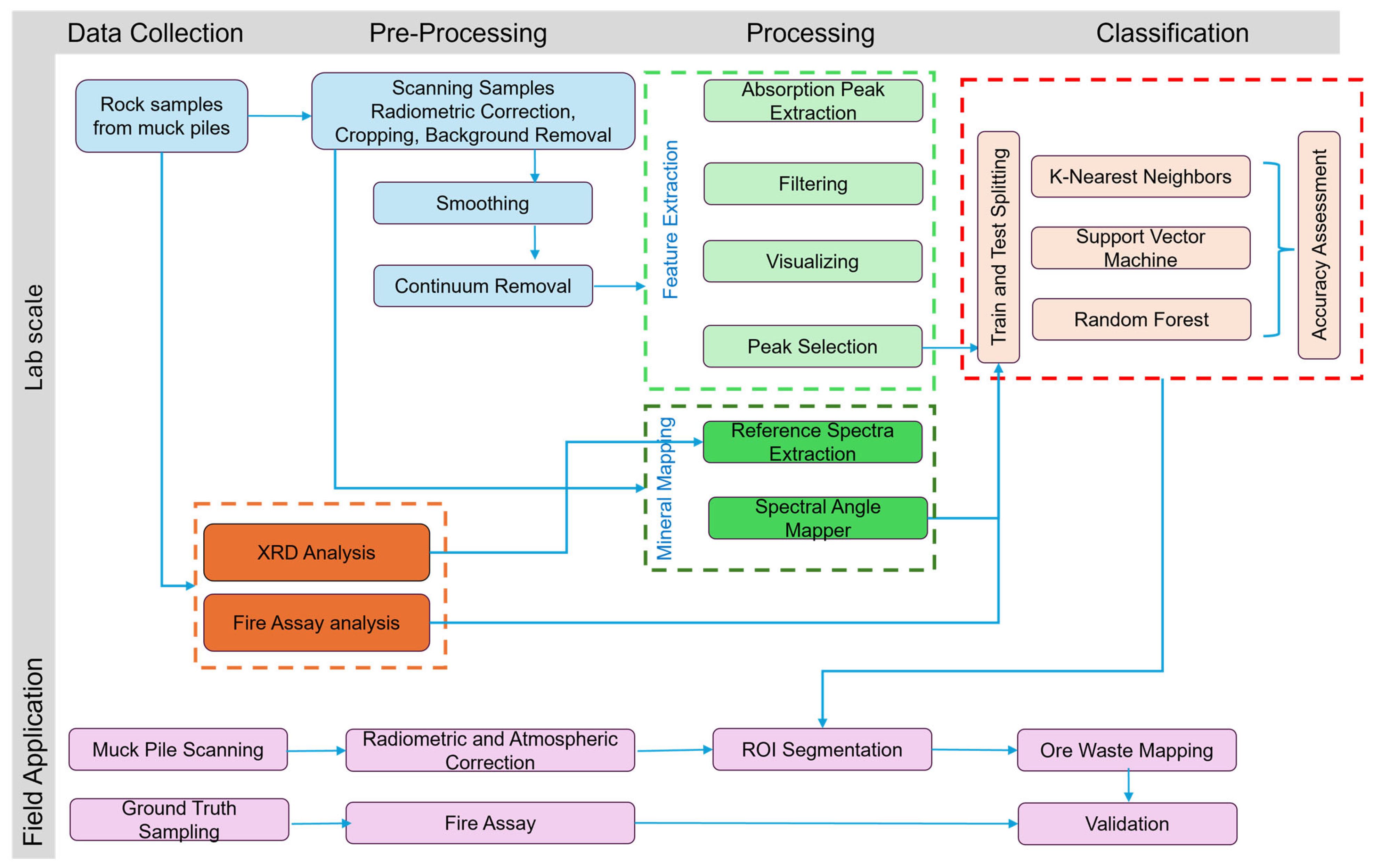
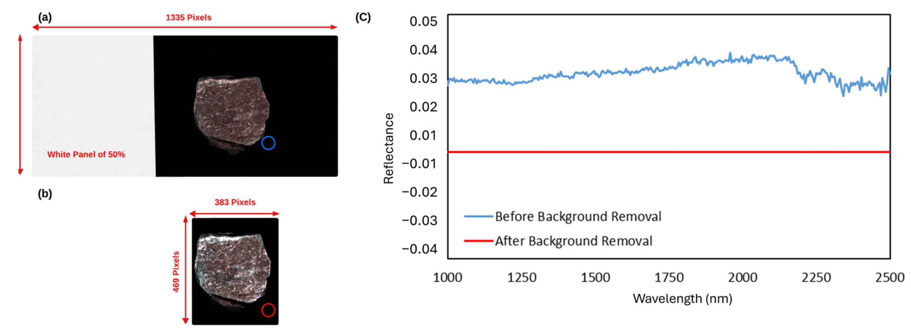
3.1.1. Data-Driven Approach: Results

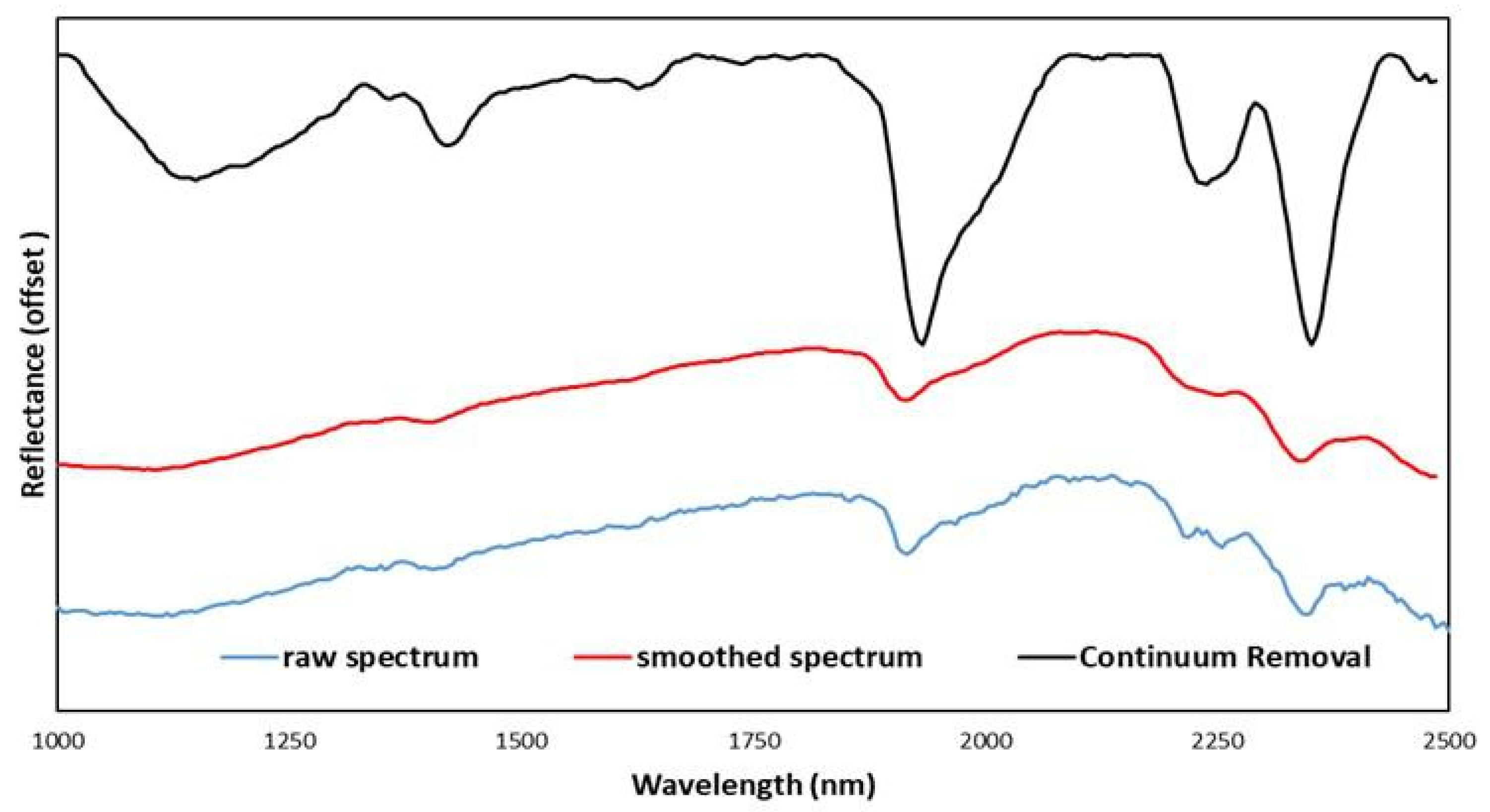
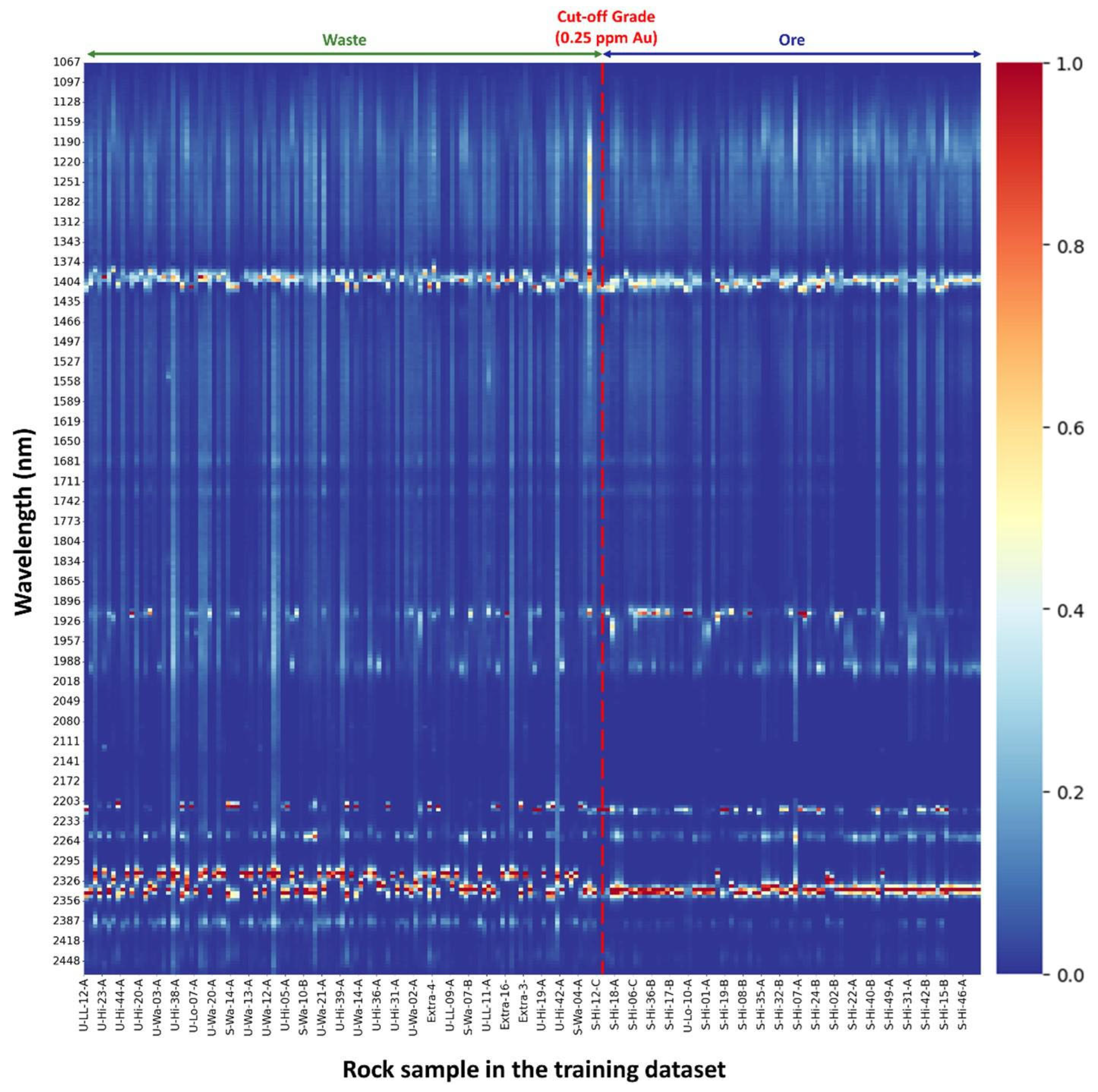
After extracting the main absorption peaks using the proposed FE approach, a heatmap was generated to visualize the distribution of the peaks across all scanned samples. Since the frequencies of the absorption peaks could vary significantly from one wavelength to another, it was impossible to distinguish the existing pattern within a wavelength with lower frequencies when other wavelengths had higher frequency values. To address this issue, we normalized the frequencies of all samples within each wavelength to between 0 and 1, as shown in Figure 11. The Y-axis represents all wavelengths, while the X-axis displays scanned samples sorted from low grade on the left to high grade on the right, with a vertical red line indicating the cut-off grade threshold. Colors on the heatmap signify the normalized frequencies of each extracted absorption peak. The generated heatmap could be used to visually inspect existing patterns within absorption peaks at a specific wavelength to discriminate between ore and waste samples. Notably, four prominent areas are observed around 1916 nm, 2208 nm, 2315 nm, and 2336 nm. It is recognized that these features were extracted based on a limited number of samples tested for the study, and they are only valid for rock samples with a similar mineralogical composition. 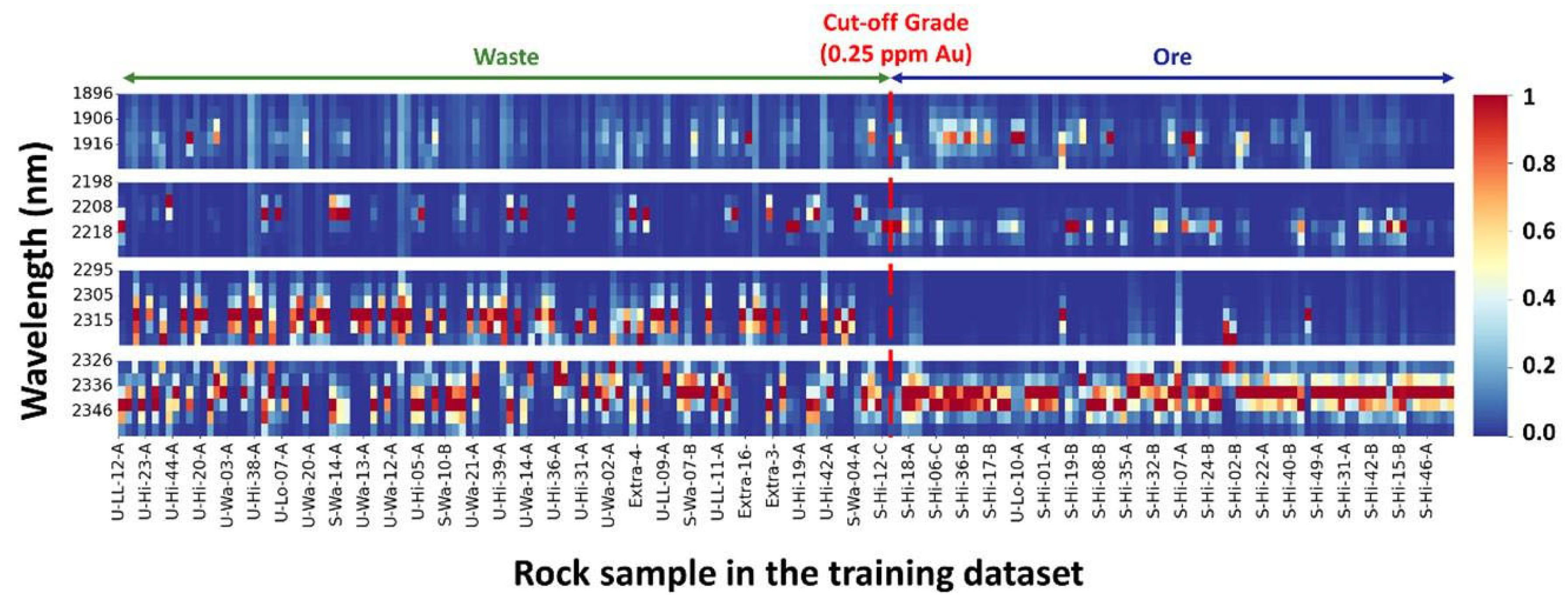Figure 12 provides a detailed view of these prominent areas, assisting in further analysis and interpretation.

Based on the detailed heatmap shown in Figure 12, it becomes apparent that certain features, such as those around 1916 nm, show a higher frequency in ore samples compared to waste samples, although the distinction is less evident than what is observed at 2208 nm. At 2208 nm, there is a clear discrimination between ore and waste samples, with waste samples exhibiting higher absorption frequencies. Similarly, at 2310 nm and 2315 nm, there is a noticeable increase in frequencies in some waste samples compared to ore samples. Features at 2336 nm and 2341 nm also show potential for discriminating between ore and waste, although with less certainty than those at 2203 nm, 2208 nm, 2310 nm, and 2315 nm. Notably, while these features may help to distinguish waste samples, they do not exhibit a consistent pattern in ore samples, making it easier to identify waste samples based solely on these features.

However, visually focusing on these extracted absorption peaks may be less helpful in identifying ore samples, as the patterns are less distinct than waste samples. While these features provide valuable insights, additional analysis and techniques may be required to identify ore samples accurately. Therefore, we utilized all extracted spectral absorption features for classification purposes, employing three popular classifiers in the remote-sensing field: RFC, SVC, and KNNC. Subsequently, the outcomes of these classifications will be presented in the following sections, showing how well they can discriminate ore and waste samples.

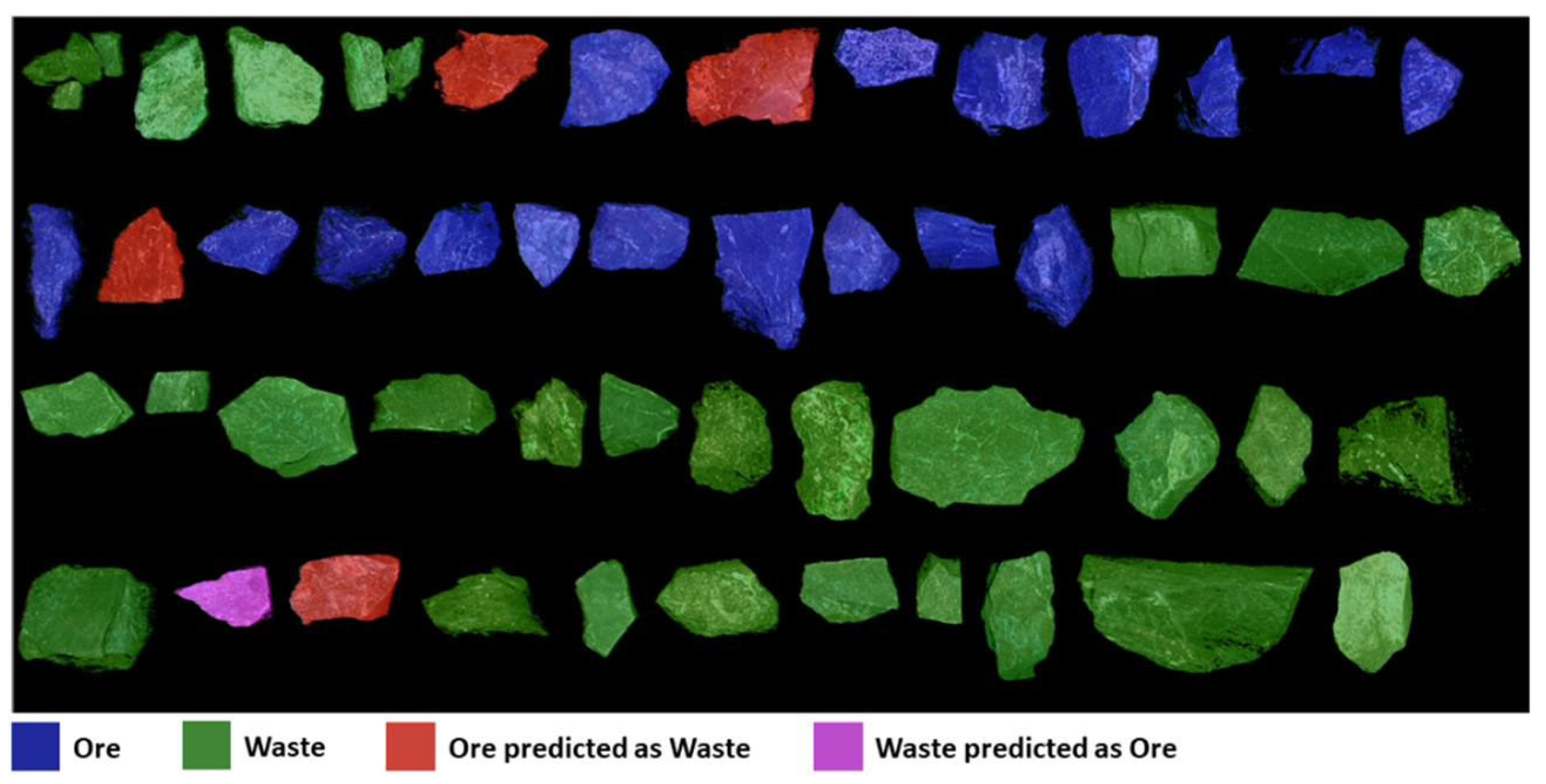
The classification process was conducted on a dataset of 196 train image samples and 50 test image samples, utilizing the extracted absorption peaks as input features. Figure 13 displays the classified output using the RFC on the testing dataset. Our analysis indicated that out of the 50 test image samples, 1 sample that was predicted as ore was, in fact, waste (highlighted in purple). Also, four samples were classified as waste, which were actually ore (highlighted in red). Additionally, the classifier accurately predicted 45 samples: 17 ore (highlighted in blue) and 28 waste (highlighted in green).

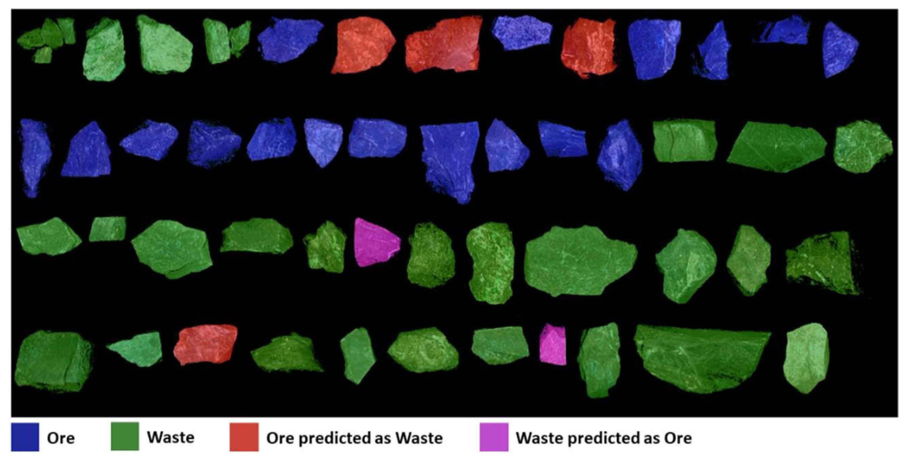
Similarly, Figure 14 illustrates the classified output using SVC on the testing dataset. The analysis showed that out of the 50 test samples, 2 samples predicted as ore were, in fact, waste (purple), while 4 samples classified as waste were ore samples (red). Furthermore, the classifier accurately predicted 44 samples, including 17 ore (blue) and 27 waste samples (green).

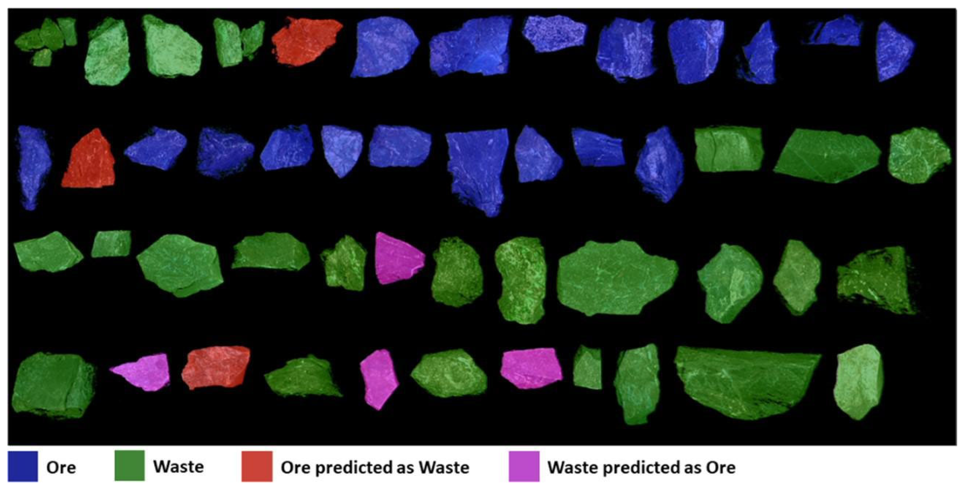
Lastly, Figure 15 demonstrates the results obtained from the KNNC applied to the testing dataset. Our examination revealed that, out of the 50 test samples, 4 samples initially classified as ore were waste samples (purple). In comparison, three samples classified as waste by the classifier were ore samples (red). Despite these discrepancies, the KNNC achieved an overall accurate prediction for 43 samples, with 18 correctly identified as ore (blue) and 25 as waste (green). These detailed analyses provide valuable insights into the performance and reliability of each classifier in accurately classifying ore and waste samples.

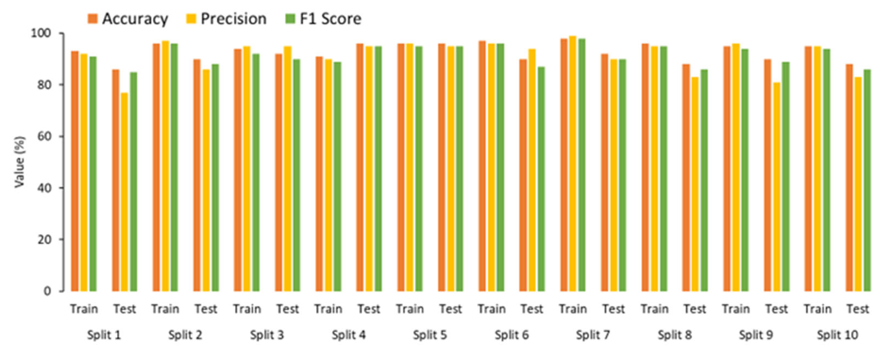
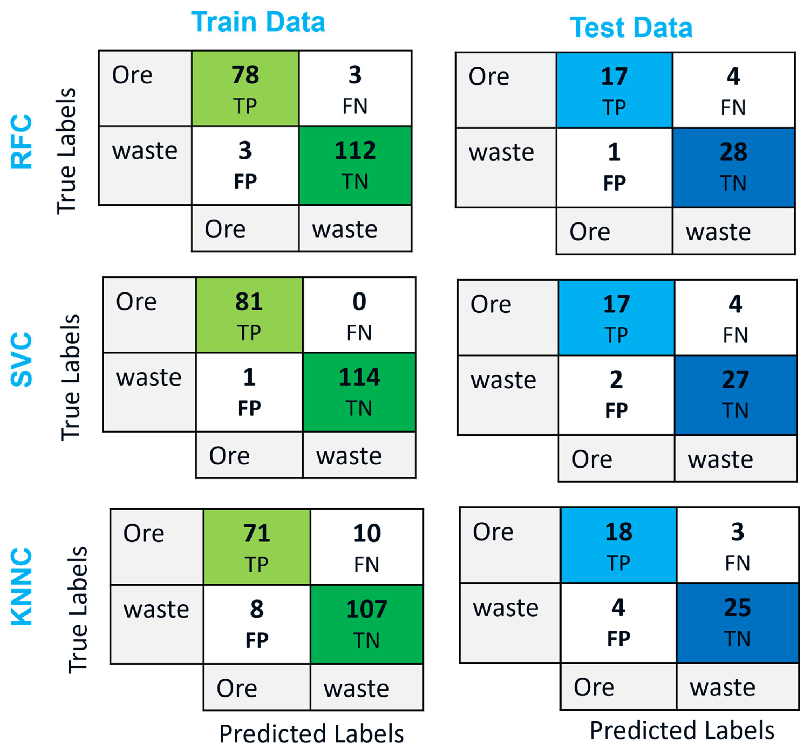
The performance of proposed classifiers was examined through a comprehensive accuracy assessment using accuracy, precision, recall, and F1-score. Figure 16 presents confusion matrices for the training and test datasets across three classifiers: RFC, SVC, and KNNC models. Additionally,

Table 5. Accuracy assessment for the testing dataset across the RFC, SVC, and KNNC models.

Classifier	Class	Overall Accuracy	Precision	Recall	F1-Score
RFC	Ore	0.90	0.94	0.81	0.87
	Waste		0.88	0.96	0.95
SVC	Ore	0.88	0.94	0.81	0.85
	Waste		0.90	0.93	0.90
KNNC	Ore	0.86	0.82	0.86	0.84
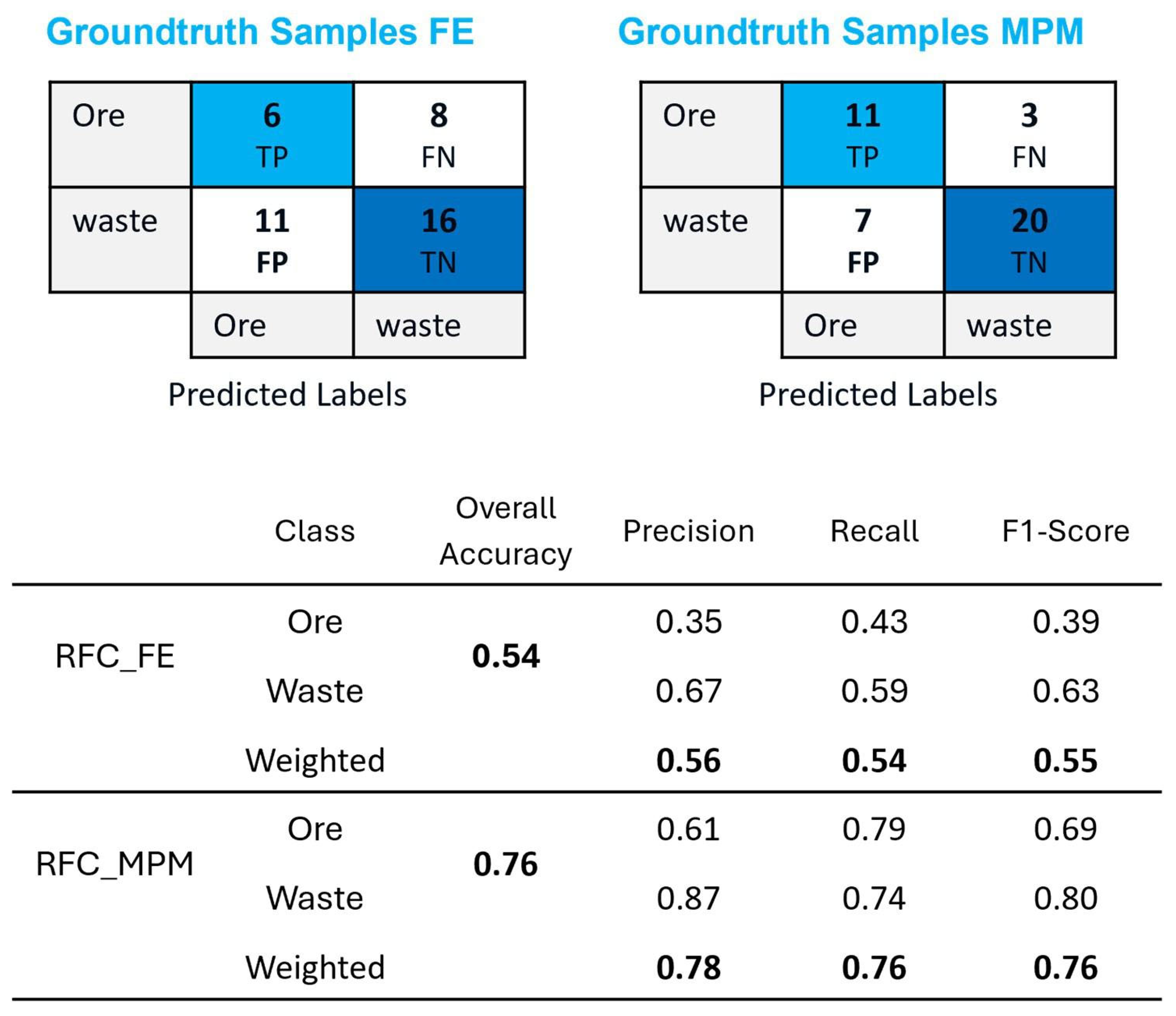
	Waste		0.89	0.86	0.88

lists the analysis of overall accuracy, precision, recall, and F1-score metrics for each classifier’s confusion matrix on the testing dataset. These assessments offer valuable insights into the classifiers’ effectiveness in accurately classifying ore and waste samples.

The results’ comparison highlights the proposed method’s effectiveness based on assessment metrics, including overall accuracy, precision, recall, and F1-score. Each metric provides valuable insights into the classifiers’ performance.

Starting with the RFC, it achieved a notable overall accuracy of 0.90, indicating that 90% of the samples were correctly classified. The high precision values for both ore, 0.94, and waste, 0.88, suggest that RFC accurately identified true positive samples for both classes. However, the recall value for ore, 0.81, indicates that some ore samples were incorrectly classified as waste, which might be attributed to a higher false negative rate. Conversely, the recall value for waste, as 0.96, suggests that RFC effectively captured the majority of true waste samples, with a lower false negative rate. The F1-score provides a great balanced measure of the classifier’s performance, with values of 0.87 for ore and 0.95 for waste.

Moving on to SVC, it resulted in an overall accuracy of 0.88, with precision values of 0.94 for ore and 0.90 for waste. Like RFC, SVC exhibited a higher precision for ore, indicating a lower false positive rate for ore samples. The recall values for both ore, 0.81, and waste, 0.93, suggest that SVM effectively captured true positive samples for waste classes like RFC did. The F1-scores for ore and waste were 0.85 and 0.90, respectively, indicating a good balance between precision and recall for both classes.

Lastly, KNNC reached an overall accuracy of 0.86, with precision values of 0.82 for ore and 0.89 for waste. The lower precision for ore suggests a higher false positive rate for ore samples compared to RFC and SVC. However, KNNC exhibited balanced recall values for both ore, 0.86, and waste, 0.86, indicating a relatively consistent performance in capturing true positive samples for both classes. The F1-scores for ore and waste were 0.84 and 0.88, respectively, indicating a good balance between precision and recall for both classes.

Regarding the F1-score and overall accuracy, RFC outperforms both SVC and KNNC, making it a suitable choice if accurately identifying both ore and waste samples is crucial. SVC exhibits higher precision than RFC and KNNC, indicating a better performance in correctly identifying positive samples. Therefore, SVC may be preferred if minimizing false positives is a priority. However, KNNC demonstrates a balanced recall for both ore and waste samples, suggesting reliability in capturing true positive samples for both classes. Thus, KNNC may be suitable if achieving a balance between capturing all positive samples is essential. Generally, while RFC may excel in overall accuracy and F1-score, SVC shows superior precision, and KNNC demonstrates balanced recall.

3.1.2. Hyperparameter Optimization

A randomized grid search was used to tune hyperparameters for each machine-learning algorithm within a five-fold cross-validation framework. This approach enhances reproducibility and ensures fair model comparison across classifiers. The final parameter values were selected based on the average validation performance across folds.

Table 6. Hyperparameter search space, optimal values, and descriptions for each classifier.

Model	Parameter	Range	Selected	Description
RFC	n_estimators	10 to 1000	707	Number of decision trees in the forest
	max_depth	1 to 50	31	Maximum depth of each decision tree
	min_samples_split	2 to 20	7	Minimum number of samples required to split an internal node
	min_samples_leaf	2 to 20	3	Minimum number of samples required at a leaf node
	max_features	0.1 to 0.9	0.55	Proportion of features considered when looking for the best split
SVC	C	0.1 to 10	1.27	Regularization parameter that balances margin size and misclassification
	gamma	‘scale’, ‘auto’	‘auto’	Kernel coefficient for non-linear decision boundaries
	kernel	‘linear’,‘poly, ‘rbf’, ‘sigmoid’	‘rbf’	Type of kernel function used to map data into higher dimensions
KNNC	n_neighbors	1 to 30	4	Number of neighbors used
	weights	‘uniform’, ‘distance’	‘uniform’	Weighting strategy applied to neighbors
	algorithm	‘auto’, ‘ball_tree’, ‘kd_tree’, ‘brute’	‘brute’	Algorithm used to compute nearest neighbors
	P	1, 2	1	1 = Manhattan, 2 = Euclidean

presents the hyperparameter search ranges explored, the optimal values obtained for each model, and a brief explanation of their roles in model behavior.

3.1.3. Overfitting Control and Model Robustness

To evaluate the robustness of the random forest classifier, we repeated the classification workflow across ten different random train–test splits. The key performance metrics—including accuracy, precision, and F1-score—remained consistent, with a coefficient of variation below 5%, as illustrated in Figure 17. This confirms the stability of the classification performance and mitigates concerns of overfitting. While more explicit regularization techniques and learning curves are typically used in neural network models, this multi-split validation strategy served as an effective control measure in our case, especially given the moderate dataset size and the inherent ensemble-based regularization characteristics of the random forest algorithm.

3.1.4. Knowledge-Based Approach: Results

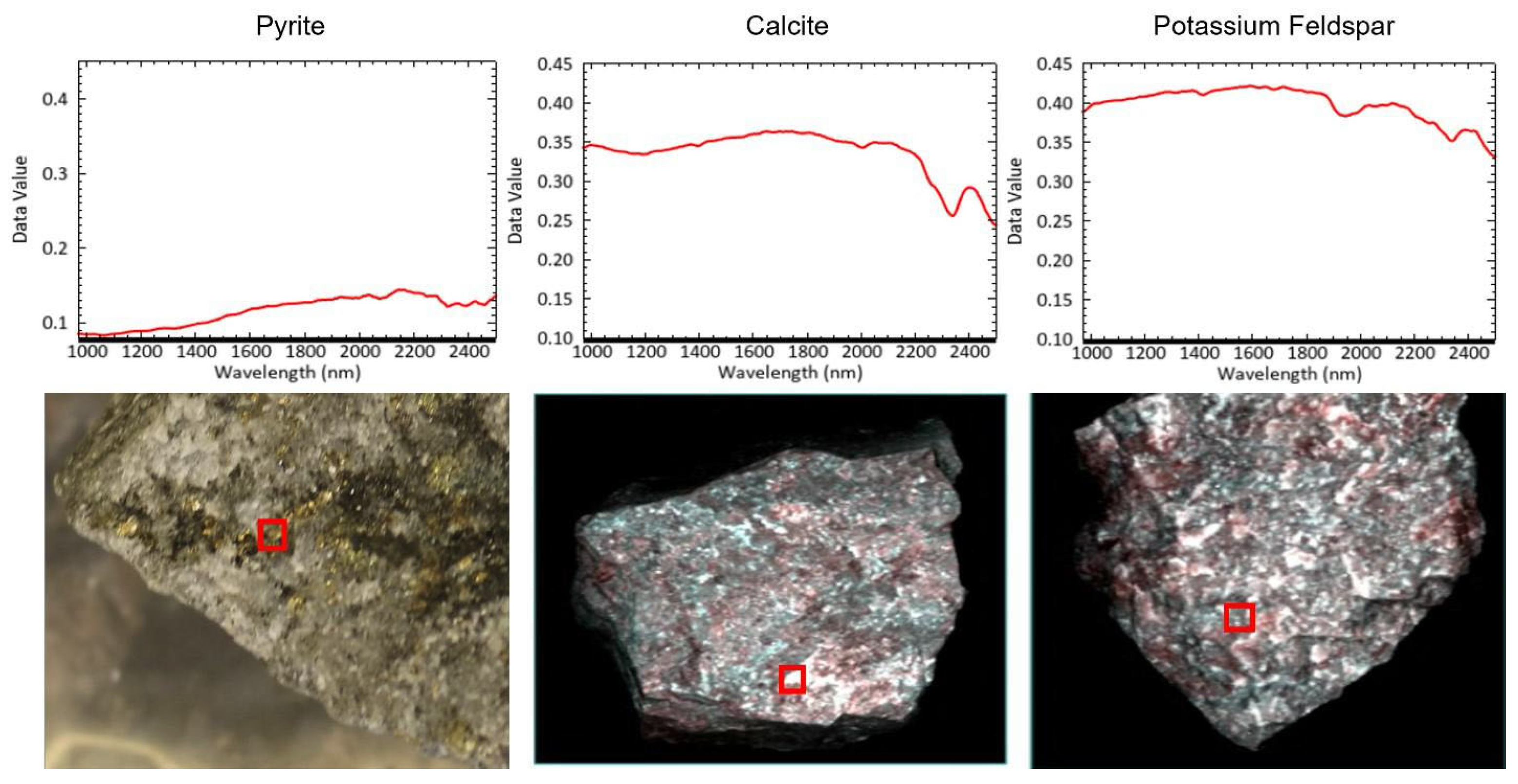
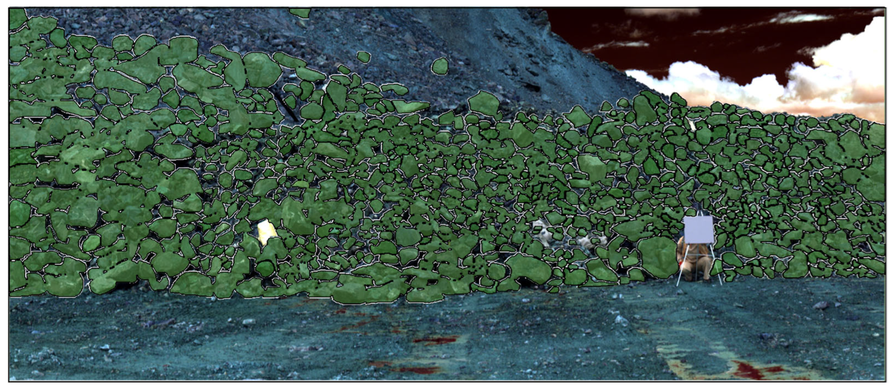
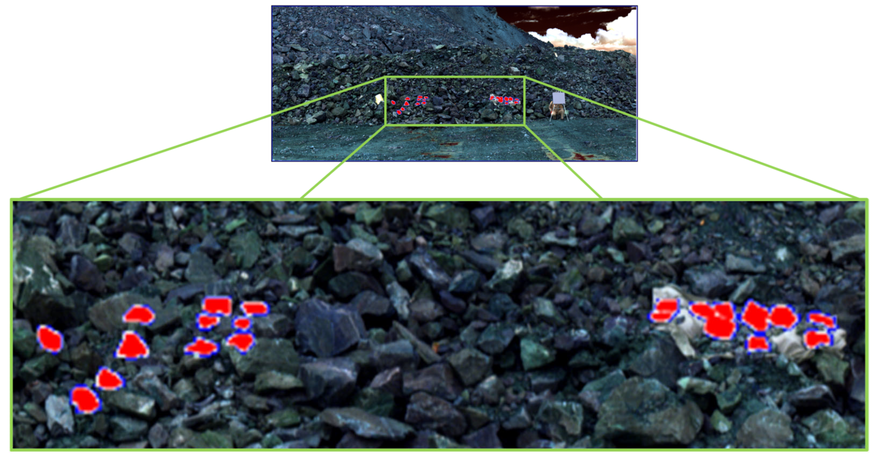
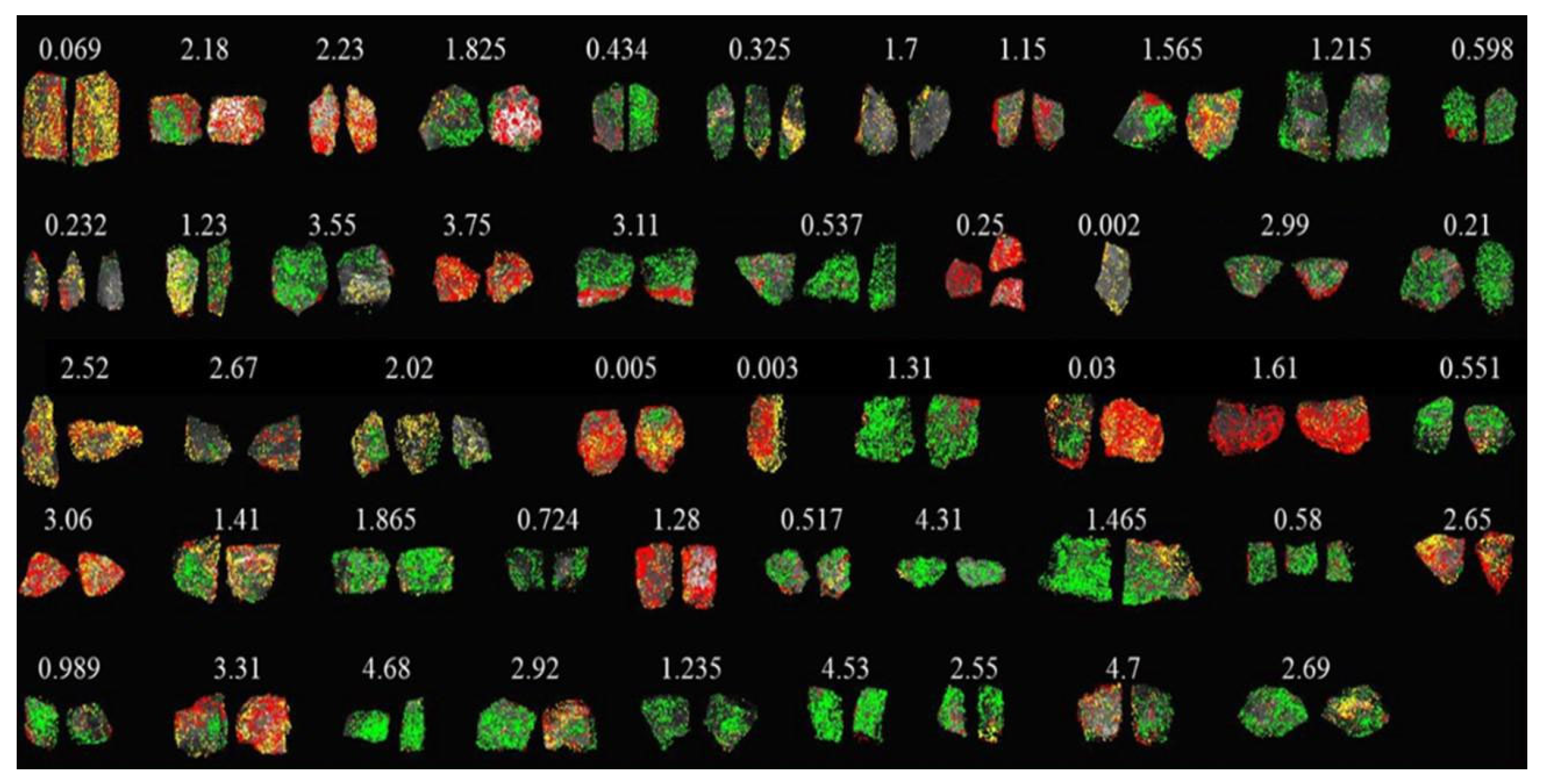
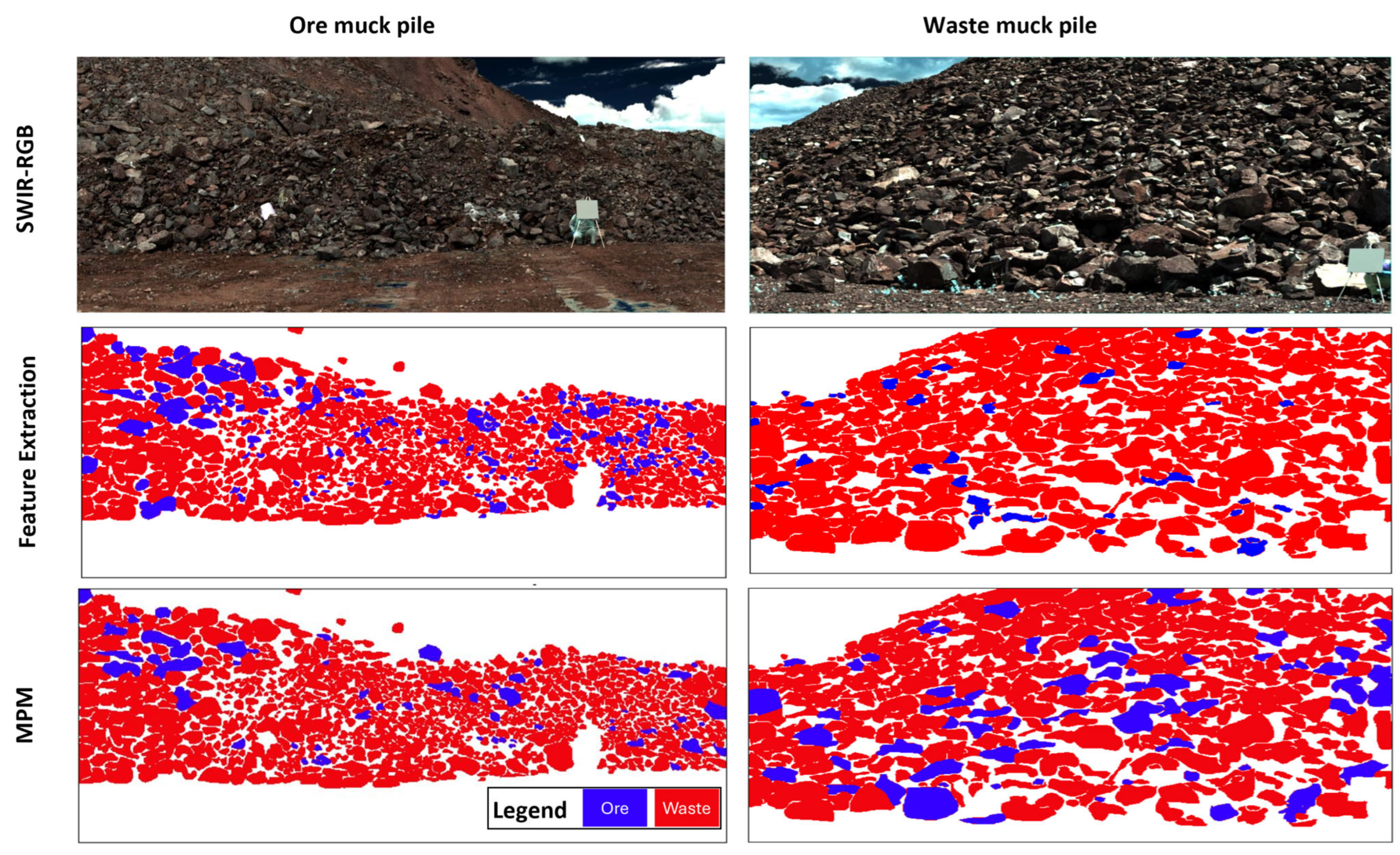
In the MPM approach, the SAM algorithm was applied to all 256 scanned hyperspectral images to classify minerals based on three local reference spectra: pyrite, calcite, and potassium feldspar. These reference spectra were extracted from laboratory-scale analysis and used to identify spectral similarities within the dataset. The MPM output generated by the SAM classification for selected images is shown in Figure 18. In these images, green pixels represent pyrite, yellow pixels represent calcite, and red pixels represent potassium feldspar. Following mineral classification, the frequency of occurrence of each mineral was calculated for each sample. These mineral abundance values were then used as input features for the classifier in the ore–waste discrimination process.

The classification process in the MPM method used the same training and testing datasets as the data-driven approach. Since RFC consistently outperformed SVC and KNNC in terms of overall accuracy and F1-score during the data-driven evaluation, it was identified as the most reliable and effective classifier. As a result, only RFC was selected for use in the MPM approach to ensure optimal performance.

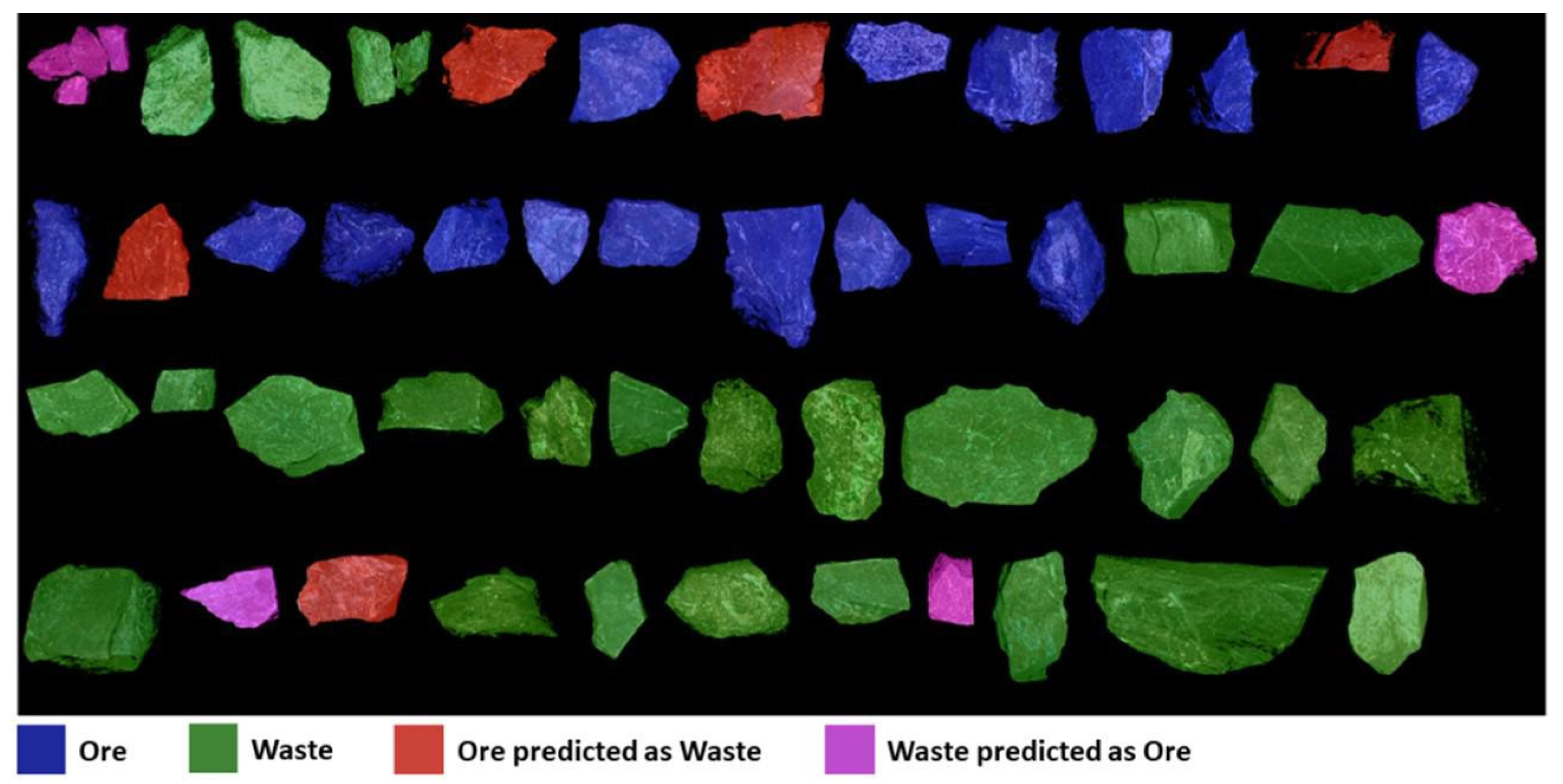
Figure 19 shows the classified output generated by the RFC model on the testing dataset. The results showed that out of the 50 test samples, 41 samples were correctly classified, including 16 ore samples, represented in blue, and 25 waste samples, represented in green. However, four samples were misclassified as ore, shown in purple, when they were actually waste, while five samples classified as waste, shown in red, were actually ore. These results demonstrate the model’s effectiveness in distinguishing ore from waste while also highlighting some misclassification cases, which could be attributed to the spectral similarities between certain ore and waste materials. 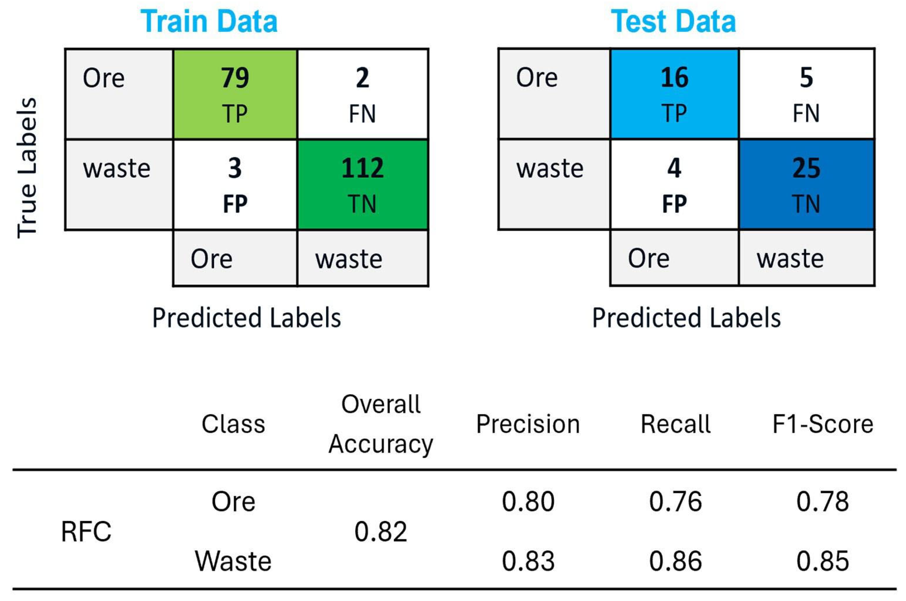Figure 20 presents the confusion matrices for the training and test datasets, along with the accuracy assessment report, to evaluate the performance of RFC in the MPM method for ore–waste discrimination.

The RFC applied in the MPM method achieved an overall accuracy of 0.82, indicating that 82% of the total samples were correctly classified. While slightly lower than the 90% accuracy achieved for RFC in the data-driven approach, this result still demonstrates a strong classification performance in distinguishing ore from waste. For the ore class, RFC obtained a precision of 0.80, meaning that 80% of the samples predicted as ore were actually ore. However, the recall of 0.76 suggests that 24% of the actual ore samples were misclassified as waste. This lower recall value indicates a relatively higher false negative rate, meaning that some ore samples were incorrectly labeled as waste. The F1-score of 0.78 represents the balance between precision and recall for ore classification, highlighting the moderate ability of the model to distinguish ore samples. In contrast, for the waste class, RFC achieved a precision of 0.83, meaning that 83% of the samples predicted as waste were truly waste. The recall value of 0.86 shows that 86% of the actual waste samples were correctly identified, with a relatively lower false negative rate compared to the ore class. The F1-score of 0.85 indicates a strong balance between precision and recall, demonstrating that the model was more effective in classifying waste than ore.

3.2. Field-Scale Results

To evaluate the performance of the developed classification models in the actual field settings, the developed algorithms were applied to the hyperspectral imagery collected from the two muck piles from the same mine, one labeled as waste and the other as ore pile. Figure 21 presents the classification results for both mock piles using both FE and MPM discrimination approaches. In these classification maps, blue-colored samples represent areas predicted as ore, while red-colored samples indicate areas classified as waste. The outputs demonstrate differences in how each method classified the materials within the piles, highlighting variations in the discrimination capabilities of the two approaches.

To validate the classification results, the 21 ground truth samples were placed on both piles, and their precise locations were recorded. The classification predictions from both methods were then compared against the fire assay results from these ground truth samples to assess the accuracy of the models.

Figure 22 illustrates the confusion matrix and accuracy assessment report for the combined classification of both muck piles, based on fire assay results. The overall classification performance was evaluated in terms of precision, recall, and F1-score for ore and waste classes.

The accuracy assessment results highlight the differences in classification performance between FE and MPM methods. The overall accuracy for MPM was recorded at 76%, whereas the FE method achieved only 54%. This indicates that MPM provides a more reliable classification, successfully identifying a greater proportion of correctly classified ore and waste samples. When evaluating the classification performance for ore, MPM demonstrated a substantial improvement over FE. The recall for ore in MPM was 0.79, compared to only 0.43 in FE, indicating that MPM correctly identified a larger proportion of the actual ore samples, thereby reducing false negatives. Similarly, the precision for ore in MPM was 0.61, while FE achieved only 0.35, meaning that FE had a higher tendency to misclassify waste as ore. The F1-score, which balances precision and recall, further reinforces the advantage of MPM, with a value of 0.69 compared to 0.39 in FE. For waste classification, MPM again outperformed FE in terms of both precision and recall. The precision for waste in MPM was recorded at 0.87, significantly higher than 0.67 in FE, suggesting that MPM was more effective in minimizing false positives when classifying waste. Additionally, MPM exhibited a recall of 0.74 compared to 0.59 in FE, indicating that it correctly identified a larger portion of actual waste samples. The F1-score for waste classification also demonstrated an improvement in MPM (0.80) over FE (0.63), confirming the higher consistency and reliability of MPM in distinguishing waste from ore.

In summary, MPM consistently demonstrated a superior performance over FE in all classification metrics. The higher accuracy, improved precision–recall balance, and reduced false positives and false negatives indicate that MPM is a more effective approach for ore–waste discrimination in this case.

To evaluate whether the classification performance differed significantly between the FE and MPM approaches, McNemar’s test was applied [56,57]. This non-parametric test is well-suited for paired nominal data, particularly for identifying performance differences between two classifiers on the same set of observations. The test focused on discordant classification outcomes: instances where one method produced a correct result while the other did not. The analysis yielded a chi-squared statistic of 5.76 with one degree of freedom, resulting in a p-value of 0.0164. As this p-value falls below the 0.05 significance threshold, the test indicates a statistically significant difference in performance between the two classifiers. Specifically, the MPM classifier correctly predicted more cases that were misclassified by the FE approach, suggesting improved classification reliability under the same conditions. These results support the conclusion that the MPM method offers a superior predictive performance and greater robustness in field-based scenarios.

4. Discussion

The findings of this study highlight the effectiveness of absorption peak extraction for discriminating between ore and waste samples in a laboratory setting. The method successfully identified distinct spectral absorption features, providing valuable insights into discrimination between ore and waste rock samples. The classification results obtained using RFC, SVC, and KNNC in the FE method demonstrated high accuracy, with RFC achieving an overall accuracy of 90%, outperforming SVC (88%) and KNNC (86%). The high precision and recall values for both ore and waste confirm that absorption peak extraction is a robust approach for hyperspectral mineral discrimination, aligning with or exceeding the performance reported in similar studies [25,29,58].

In mining applications, model evaluation must extend beyond overall accuracy to consider the economic implications of classification errors. When ore material is misclassified as waste, it leads to ore loss and lost revenue. Conversely, dilution, where waste material is misclassified as ore, results in a reduced average grade of the material and unnecessary processing costs. In our laboratory-scale test results, RFC provided the most balanced performance with minimal ore loss (four false negatives) and the lowest waste dilution (one false positive), making it the most economically favorable choice. However, the prioritization of classifiers should be aligned with site-specific economic considerations. For example, if the cost of losing high-grade ore is considerably greater than processing extra waste, a model which had the lowest ore loss but higher dilution might be preferable.

In comparing the FE and MPM methods in laboratory-scale analysis, the FE-based classification consistently outperformed MPM in terms of accuracy, precision, and recall. The FE method, particularly when coupled with RFC, exhibited an overall accuracy of 90%, demonstrating its effectiveness in distinguishing ore from waste under controlled conditions such as uniform lighting, a fixed sensor-to-sample distance, minimal background interference, and the absence of dust or moisture on sample surfaces. This superior performance can be attributed to FE’s ability to capture subtle spectral variations associated with mineralogical differences, allowing for more precise classification. In contrast, MPM, which relies on predefined spectral reference data, achieved an overall accuracy of 82% in the laboratory setting, slightly lower than FE. The lower recall observed for ore samples in MPM suggests that some ore materials were misclassified, likely due to the spectral similarity between certain ore and waste components when using resampled reference spectra. However, despite its slightly lower accuracy in the laboratory-scale analysis, MPM remained a robust method for mineral discrimination, especially for waste classification, where it exhibited higher recall values.

While FE demonstrated a superior performance in the laboratory-scale analysis, the field application results revealed a reversal in trends, with MPM outperforming FE. The overall accuracy of MPM in the field was recorded at 76%, whereas FE achieved only 54%. This performance gap can largely be attributed to the influence of environmental variations. In the field setting, variations such as inconsistent lighting, sensor-to-target distance, surface dust, and background interference introduced spectral noise, affecting the quality of the data collected. More importantly, the use of natural sunlight introduced atmospheric absorption effects, which impacted specific wavelength regions. As a result, during radiometric and atmospheric correction, certain spectral bands had to be removed. For example, strong absorption peaks at 1916 nm and 2208 nm, clearly visible in laboratory-generated heatmaps, were either partially or fully lost in the field data. This significantly reduced the discriminating power of the FE method, which depends on precise peak-based features. In contrast, MPM, which is based on spectral matching techniques like SAM, is inherently more adaptive to changes in lighting conditions, moisture, and surface roughness because it relies on relative spectral similarity rather than absolute feature intensities. On the other hand, FE’s dependence on specific spectral features makes it more susceptible to these environmental factors, leading to increased misclassification in uncontrolled field conditions. The field results highlight the limitations of FE when applied outside a controlled laboratory environment, emphasizing the need for improved preprocessing techniques and environmental correction models to enhance its robustness in real-world applications.

Hyperspectral field scanning presents a valuable opportunity for real-time, non-destructive ore–waste discrimination. While our results indicate that MPM demonstrated a stronger performance in field conditions due to its reliance on predefined spectral libraries, FE methods remain promising for automated analysis. Since FE does not require prior mineralogical knowledge, it is well-suited for real-time, adaptive classification in controlled environments, such as conveyor belt ore sorting, where lighting, sensor distance, and sample surface conditions can be tightly regulated. In such settings, the consistency of spectral acquisition ensures reliable extraction of absorption features, making FE-based classification more scalable. Conversely, MPM is more suitable for field-based applications such as mapping blasted muck piles or stockpile monitoring, where environmental variability is unavoidable but reference spectra can still facilitate accurate mineral identification. Each method thus offers unique advantages: FE provides flexibility and automation under controlled conditions, while MPM ensures interpretability and resilience in geologically complex, open-field environments.

Looking forward, research should focus on improving the robustness of FE methods under variable field conditions, including the development of adaptive preprocessing and learning techniques. Hybrid models that combine FE with knowledge-based strategies like MPM may offer a balanced solution—leveraging the adaptability of FE while maintaining the reliability of spectral libraries. Beyond methodological considerations, these findings hold direct implications for mining operations. Integrating both FE and MPM into operational workflows could reduce dependence on manual sampling, enable real-time decision-making at the muck pile or conveyor level, and optimize resource allocation. This approach has the potential to reduce dilution, enhance grade control, and streamline stockpile management, yielding both economic and environmental benefits. Ultimately, this study provides a practical foundation for deploying intelligent, non-destructive ore-sorting solutions using tailored hyperspectral strategies across a range of mining scenarios.

5. Conclusions

This study evaluated the performance of data-driven and knowledge-based classifiers for ore–waste discrimination using hyperspectral SWIR data under both controlled laboratory and actual mine site conditions. A total of 178 rock samples were collected and scanned in a laboratory environment, and two muck piles were analyzed for field testing. The data-driven method, based on absorption peak extraction, achieved strong classification results in the laboratory setting, with overall accuracies ranging from 0.86 to 0.90 and F1-scores between 0.84 and 0.95 across three classifiers (RFC, SVC, and KNNC). These results emphasize the reliability of this approach in capturing critical spectral features while maintaining a robust balance between precision and recall. In contrast, the knowledge-based MPM approach yielded lower F1-scores of 0.78 and 0.85 under the same laboratory conditions, indicating that the absorption peak method offers superior performance in controlled environments where spectral quality is high.

The data-driven method showed promise for real-time, automated ore–waste discrimination, eliminating the need for predefined mineralogical rules, making it suitable for large-scale or near-real-time deployments. However, its performance was more susceptible to spectral inconsistencies caused by variable lighting, surface roughness, and sensor noise. These issues underscore the importance of future research on more robust preprocessing techniques, such as adaptive continuum removal and denoising, as well as the development of models that can adapt to changing field conditions.

Conversely, the knowledge-based MPM approach, which depends on expert-defined decision criteria and known mineral spectral signatures, proved far more reliable under challenging field conditions. It maintained stable classification even when raw spectra were noisy or affected by environmental variability. This strength makes it a suitable choice for operational environments, but it comes with some limitations; it requires prior mineralogical knowledge, and reduced adaptability to unknown materials or spectral patterns.

The ability of hyperspectral remote sensing to provide non-destructive, real-time mineral analysis offers substantial operational advantages by decreasing reliance on manual sampling and enhancing ore–waste delineation, resource allocation, and waste management strategies. While the proposed dual-method framework shows strong performance within a hydrothermally altered gold deposit, its generalization to other geological settings should be approached with caution, as the spectral characteristics are site-specific. Additionally, only a subset of the available data was utilized, certain spectral regions were excluded due to noise, and the sampling coverage was spatially limited. Future research should focus on optimizing peak extraction for field conditions, integrating spectral correction models, and validating the approach across diverse types of deposits. Advancing hybrid methods that combine data-driven and knowledge-based strategies will further support the efficient, accurate, and sustainable application of hyperspectral imaging in mining operations.

References

1. Lessard, J.; de Bakker, J.; McHugh, L. Development of Ore Sorting and Its Impact on Mineral Processing Economics. Miner. Eng. 2014, 65, 88–97. [Google Scholar] [CrossRef]
2. Desta, F.; Buxton, M. Image and Point Data Fusion for Enhanced Discrimination of Ore and Waste in Mining. Minerals 2020, 10, 1110. [Google Scholar] [CrossRef]
3. Isaaks, E.; Treloar, I.; Elenbaas, T. Optimum Dig Lines for Open Pit Grade Control. In Proceedings of the 9th International Mining Geology Conference, Adelaide, Australia, 10–11 June 2014; Australasian Institute of Mining and Metallurgy: Melbourne, Australia, 2014; pp. 425–532. [Google Scholar]
4. Abdolmaleki, M.; Consens, M.; Esmaeili, K. Ore-Waste Discrimination Using Supervised and Unsupervised Classification of Hyperspectral Images. Remote Sens. 2022, 14, 6386. [Google Scholar] [CrossRef]
5. Abrams, M.J.; Ashley, R.P.; Rowan, L.C.; Goetz, A.F.H.; Kahle, A.B. Mapping of Hydrothermal Alteration in the Cuprite Mining District, Nevada, Using Aircraft Scanner Images for the Spectral Region 0.46 to 2.36 µm. Geology 1977, 5, 713. [Google Scholar] [CrossRef]
6. Riaza, A.; Strobl, P.; Beisl, U.; Hausold, A.; Müller, A. Spectral Mapping of Rock Weathering Degrees on Granite Using Hyperspectral DAIS 7915 Spectrometer Data. Int. J. Appl. Earth Obs. Geoinf. 2001, 3, 345–354. [Google Scholar] [CrossRef]
7. Baissa, R.; Labbassi, K.; Launeau, P.; Gaudin, A.; Ouajhain, B. Using HySpex SWIR-320m Hyperspectral Data for the Identification and Mapping of Minerals in Hand Specimens of Carbonate Rocks from the Ankloute Formation (Agadir Basin, Western Morocco). J. Afr. Earth Sci. 2011, 61, 1–9. [Google Scholar] [CrossRef]
8. Mathieu, M.; Roy, R.; Launeau, P.; Cathelineau, M.; Quirt, D. Alteration Mapping on Drill Cores Using a HySpex SWIR-320m Hyperspectral Camera: Application to the Exploration of an Unconformity-Related Uranium Deposit (Saskatchewan, Canada). J. Geochem. Explor. 2017, 172, 71–88. [Google Scholar] [CrossRef]
9. Lorenz, S.; Kirsch, M.; Zimmermann, R.; Tusa, L.; Mockel, R.; Chamberland, M.; Gloaguen, R. Long-Wave Hyperspectral Imaging for Lithological Mapping: A Case Study. In Proceedings of the IGARSS 2008—2018 IEEE International Geoscience and Remote Sensing Symposium; IEEE: Piscataway, NJ, USA, 2018; pp. 1620–1623. [Google Scholar]
10. Bou-Orm, N.; AlRomaithi, A.A.; Elrmeithi, M.; Ali, F.M.; Nazzal, Y.; Howari, F.M.; Al Aydaroos, F. Advantages of First-Derivative Reflectance Spectroscopy in the VNIR-SWIR for the Quantification of Olivine and Hematite. Planet Space Sci. 2020, 188, 104957. [Google Scholar] [CrossRef]
11. Ghadernejad, S.; Esmaeili, K. Predicting Rock Hardness and Abrasivity Using Hyperspectral Imaging Data and Random Forest Regressor Model. Remote Sens. 2024, 16, 3778. [Google Scholar] [CrossRef]
12. Dalm, M.; Buxton, M.W.N.; van Ruitenbeek, F.J.A. Ore–Waste Discrimination in Epithermal Deposits Using Near-Infrared to Short-Wavelength Infrared (NIR-SWIR) Hyperspectral Imagery. Math Geosci. 2019, 51, 849–875. [Google Scholar] [CrossRef]
13. Lypaczewski, P.; Rivard, B.; Gaillard, N.; Perrouty, S.; Piette-Lauzière, N.; Bérubé, C.L.; Linnen, R.L. Using Hyperspectral Imaging to Vector towards Mineralization at the Canadian Malartic Gold Deposit, Québec, Canada. Ore Geol. Rev. 2019, 111, 102945. [Google Scholar] [CrossRef]
14. Tuşa, L.; Kern, M.; Khodadadzadeh, M.; Blannin, R.; Gloaguen, R.; Gutzmer, J. Evaluating the Performance of Hyperspectral Short-Wave Infrared Sensors for the Pre-Sorting of Complex Ores Using Machine Learning Methods. Miner. Eng. 2020, 146, 106150. [Google Scholar] [CrossRef]
15. El Mansour, A.; Laamrani, A.; Elghali, A.; Hakkou, R.; Benzaazoua, M. A Cutting-Edge Framework for Sustainable Phosphate Waste Characterization Using Hyperspectral Imaging and Machine Learning. In Proceedings of the European Geosciences Union (EGU), Vienna, Austria, 15 March 2025. [Google Scholar]
16. Zhang, H.; Duan, L.; Zhang, Y.; Li, H.; Li, D.; Li, Y. Applicability Analysis with the Improved Spectral Unmixing Models Based on the Measured Hyperspectral Data of Mixed Minerals. Minerals 2025, 15, 715. [Google Scholar] [CrossRef]
17. Vapnik, V.N. An Overview of Statistical Learning Theory. IEEE Trans. Neural. Netw. 1999, 10, 988–999. [Google Scholar] [CrossRef] [PubMed]
18. Breiman, L. Random Forests. Mach. Learn. 2001, 45, 5–32. [Google Scholar] [CrossRef]
19. Fix, E.; Hodges, J.L. Discriminatory Analysis, Nonparametric Discrimination: Consistency Properties; International Statistical Institute: The Hague, The Netherlands, 1951. [Google Scholar]
20. Murphy, R.J.; Monteiro, S.T.; Schneider, S. Evaluating Classification Techniques for Mapping Vertical Geology Using Field-Based Hyperspectral Sensors. IEEE Trans. Geosci. Remote Sens. 2012, 50, 3066–3080. [Google Scholar] [CrossRef]
21. Zhang, N.; Zhou, K.; Li, D. Back-Propagation Neural Network and Support Vector Machines for Gold Mineral Prospectivity Mapping in the Hatu Region, Xinjiang, China. Earth Sci. Inform. 2018, 11, 553–566. [Google Scholar] [CrossRef]
22. Ghezelbash, R.; Maghsoudi, A.; Carranza, E.J.M. Performance Evaluation of RBF- and SVM-Based Machine Learning Algorithms for Predictive Mineral Prospectivity Modeling: Integration of S-A Multifractal Model and Mineralization Controls. Earth Sci. Inform. 2019, 12, 277–293. [Google Scholar] [CrossRef]
23. Krupnik, D.; Khan, S.D. High-Resolution Hyperspectral Mineral Mapping: Case Studies in the Edwards Limestone, Texas, USA and Sulfide-Rich Quartz Veins from the Ladakh Batholith, Northern Pakistan. Minerals 2020, 10, 967. [Google Scholar] [CrossRef]
24. Mondal, S.; Guha, A.; Kumar Pal, S. Support Vector Machine-Based Integration of AVIRIS NG Hyperspectral and Ground Geophysical Data for Identifying Potential Zones for Chromite Exploration—A Study in Tamil Nadu, India. Adv. Space Res. 2024, 73, 1475–1490. [Google Scholar] [CrossRef]
25. Wang, S.; Zhou, K.; Wang, J.; Zhao, J. Identifying and Mapping Alteration Minerals Using HySpex Airborne Hyperspectral Data and Random Forest Algorithm. Front. Earth Sci. 2022, 10, 871529. [Google Scholar] [CrossRef]
26. Contreras, I.C.; Khodadadzadeh, M.; Gloaguen, R. Multi-label classification for drill-core hyperspectral mineral mapping. Int. Arch. Photogramm. Remote Sens. Spat. Inf. Sci. 2020, XLIII-B3-2020, 383–388. [Google Scholar] [CrossRef]
27. Lachaud, A.; Adam, M.; Mišković, I. Comparative Study of Random Forest and Support Vector Machine Algorithms in Mineral Prospectivity Mapping with Limited Training Data. Minerals 2023, 13, 1073. [Google Scholar] [CrossRef]
28. Shebl, A.; Abriha, D.; Fahil, A.S.; El-Dokouny, H.A.; Elrasheed, A.A.; Csámer, Á. PRISMA Hyperspectral Data for Lithological Mapping in the Egyptian Eastern Desert: Evaluating the Support Vector Machine, Random Forest, and XG Boost Machine Learning Algorithms. Ore Geol. Rev. 2023, 161, 105652. [Google Scholar] [CrossRef]
29. Tsubomatsu, H.; Tonooka, H. Region Expansion of a Hyperspectral-Based Mineral Map Using Random Forest Classification with Multispectral Data. Minerals 2023, 13, 754. [Google Scholar] [CrossRef]
30. Cracknell, M.J.; Reading, A.M. Geological Mapping Using Remote Sensing Data: A Comparison of Five Machine Learning Algorithms, Their Response to Variations in the Spatial Distribution of Training Data and the Use of Explicit Spatial Information. Comput. Geosci. 2014, 63, 22–33. [Google Scholar] [CrossRef]
31. Wang, H.; Wang, J. The Multi-Objective Optimization of Tunneling Boring Machine Control Based on Geological Conditions Identification. J. Intell. Manuf. Spec. Equip. 2020, 1, 87–105. [Google Scholar] [CrossRef]
32. Hajaj, S.; El Harti, A.; Jellouli, A.; Pour, A.B.; Mnissar Himyari, S.; Hamzaoui, A.; Hashim, M. Evaluating the Performance of Machine Learning and Deep Learning Techniques to HyMap Imagery for Lithological Mapping in a Semi-Arid Region: Case Study from Western Anti-Atlas, Morocco. Minerals 2023, 13, 766. [Google Scholar] [CrossRef]
33. Acosta, I.C.C.; Khodadadzadeh, M.; Tusa, L.; Ghamisi, P.; Gloaguen, R. A Machine Learning Framework for Drill-Core Mineral Mapping Using Hyperspectral and High-Resolution Mineralogical Data Fusion. IEEE J. Sel. Top Appl. Earth Obs. Remote Sens. 2019, 12, 4829–4842. [Google Scholar] [CrossRef]
34. Thiele, S.T.; Lorenz, S.; Kirsch, M.; Cecilia Contreras Acosta, I.; Tusa, L.; Herrmann, E.; Möckel, R.; Gloaguen, R. Multi-Scale, Multi-Sensor Data Integration for Automated 3-D Geological Mapping. Ore Geol. Rev. 2021, 136, 104252. [Google Scholar] [CrossRef]
35. Kurz, T.H.; Buckley, S.J.; Howell, J.A. Close-Range Hyperspectral Imaging for Geological Field Studies: Workflow and Methods. Int. J. Remote Sens. 2013, 34, 1798–1822. [Google Scholar] [CrossRef]
36. Abdolmaleki, M.; Tabaei, M.; Fathianpour, N.; Gorte, B.G.H. Selecting Optimum Base Wavelet for Extracting Spectral Alteration Features Associated with Porphyry Copper Mineralization Using Hyperspectral Images. Int. J. Appl. Earth Obs. Geoinf. 2017, 58, 134–144. [Google Scholar] [CrossRef]
37. Lorenz, S.; Salehi, S.; Kirsch, M.; Zimmermann, R.; Unger, G.; Vest Sørensen, E.; Gloaguen, R. Radiometric Correction and 3D Integration of Long-Range Ground-Based Hyperspectral Imagery for Mineral Exploration of Vertical Outcrops. Remote Sens. 2018, 10, 176. [Google Scholar] [CrossRef]
38. Xiao, B.; Chu, G.; Feng, Y. Short-Wave Infrared (SWIR) Spectral and Geochemical Characteristics of Hydrothermal Alteration Minerals in the Laowangou Au Deposit: Implications for Ore Genesis and Vectoring. Ore Geol. Rev. 2021, 139, 104463. [Google Scholar] [CrossRef]
39. Abdolmaleki, M.; Fathianpour, N.; Tabaei, M. Evaluating the Performance of the Wavelet Transform in Extracting Spectral Alteration Features from Hyperspectral Images. Int. J. Remote Sens. 2018, 39, 6076–6094. [Google Scholar] [CrossRef]
40. van der Meer, F.D.; van der Werff, H.M.A.; van Ruitenbeek, F.J.A.; Hecker, C.A.; Bakker, W.H.; Noomen, M.F.; van der Meijde, M.; Carranza, E.J.M.; de Smeth, J.B.; Woldai, T. Multi- and Hyperspectral Geologic Remote Sensing: A Review. Int. J. Appl. Earth Obs. Geoinf. 2012, 14, 112–128. [Google Scholar] [CrossRef]
41. Lypaczewski, P.; Rivard, B. Estimating the Mg# and AlVI Content of Biotite and Chlorite from Shortwave Infrared Reflectance Spectroscopy: Predictive Equations and Recommendations for Their Use. Int. J. Appl. Earth Obs. Geoinf. 2018, 68, 116–126. [Google Scholar] [CrossRef]
42. Duke, E.F. Near Infrared Spectra of Muscovite, Tschermak Substitution, and Metamorphic Reaction Progress: Implications for Remote Sensing. Geology 1994, 22, 621. [Google Scholar] [CrossRef]
43. Clark, R.N.; King, T.V.V.; Klejwa, M.; Swayze, G.A.; Vergo, N. High Spectral Resolution Reflectance Spectroscopy of Minerals. J. Geophys. Res. Solid Earth 1990, 95, 12653–12680. [Google Scholar] [CrossRef]
44. Guo, Y.; Han, S.; Li, Y.; Zhang, C.; Bai, Y. K-Nearest Neighbor Combined with Guided Filter for Hyperspectral Image Classification. Procedia Comput. Sci. 2018, 129, 159–165. [Google Scholar] [CrossRef]
45. Breiman, L. Bagging Predictors. Mach. Learn. 1996, 24, 123–140. [Google Scholar] [CrossRef]
46. Waske, B.; Braun, M. Classifier Ensembles for Land Cover Mapping Using Multitemporal SAR Imagery. ISPRS J. Photogramm. Remote Sens. 2009, 64, 450–457. [Google Scholar] [CrossRef]
47. Wang, J.; Zuo, R.; Xiong, Y. Mapping Mineral Prospectivity via Semi-Supervised Random Forest. Nat. Resour. Res. 2020, 29, 189–202. [Google Scholar] [CrossRef]
48. Vapnik, V.N.; Vapnik, V. Statistical Learning Theory; Springer: Berlin/Heidelberg, Germany, 1998. [Google Scholar]
49. Hsu, T.-C.; Wang, T.-Y.; Hong, Y.-W.P. Collaborative Change Detection for Efficient Spectrum Sensing in Cognitive Radio Networks. In Proceedings of the 2010 IEEE 71st Vehicular Technology Conference; IEEE: Piscataway, NJ, USA, 2010; pp. 1–5. [Google Scholar]
50. Akbulut, Y.; Sengur, A.; Guo, Y.; Smarandache, F. NS-k-NN: Neutrosophic Set-Based k-Nearest Neighbors Classifier. Symmetry 2017, 9, 179. [Google Scholar] [CrossRef]
51. Thanh Noi, P.; Kappas, M. Comparison of Random Forest, k-Nearest Neighbor, and Support Vector Machine Classifiers for Land Cover Classification Using Sentinel-2 Imagery. Sensors 2017, 18, 18. [Google Scholar] [CrossRef]
52. Pacheco, A.d.P.; Junior, J.A.d.S.; Ruiz-Armenteros, A.M.; Henriques, R.F.F. Assessment of K-Nearest Neighbor and Random Forest Classifiers for Mapping Forest Fire Areas in Central Portugal Using Landsat-8, Sentinel-2, and Terra Imagery. Remote Sens. 2021, 13, 1345. [Google Scholar] [CrossRef]
53. Zhang, P.; Xu, C.; Ma, S.; Shao, X.; Tian, Y.; Wen, B. Automatic Extraction of Seismic Landslides in Large Areas with Complex Environments Based on Deep Learning: An Example of the 2018 Iburi Earthquake, Japan. Remote Sens. 2020, 12, 3992. [Google Scholar] [CrossRef]
54. Fetai, B.; Račič, M.; Lisec, A. Deep Learning for Detection of Visible Land Boundaries from UAV Imagery. Remote Sens. 2021, 13, 2077. [Google Scholar] [CrossRef]
55. Liu, L.-Y.; Wang, C.-K. Building segmentation in agricultural land using high resolution satellite imagery based on deep learning approach. Int. Arch. Photogramm. Remote Sens. Spat. Inf. Sci. 2021, XLIII-B3-2021, 587–594. [Google Scholar] [CrossRef]
56. Foody, G.M. Classification Accuracy Comparison: Hypothesis Tests and the Use of Confidence Intervals in Evaluations of Difference, Equivalence and Non-Inferiority. Remote Sens. Environ. 2009, 113, 1658–1663. [Google Scholar] [CrossRef]
57. Demšar, J. Statistical Comparisons of Classifiers over Multiple Data Sets. J. Mach. Learn. Res. 2006, 7, 1–30. [Google Scholar]
58. Hamedianfar, A.; Laakso, K.; Middleton, M.; Törmänen, T.; Köykkä, J.; Torppa, J. Leveraging High-Resolution Long-Wave Infrared Hyperspectral Laboratory Imaging Data for Mineral Identification Using Machine Learning Methods. Remote Sens. 2023, 15, 4806. [Google Scholar] [CrossRef]
Figure 1. Laboratory hyperspectral imaging setup.
Minerals 15 00741 g001
Figure 2. Field hyperspectral imaging setup scanning a pile labeled as waste in the mine.
Minerals 15 00741 g002
Figure 3. Workflow for ore and waste classification based on the proposed absorption feature extraction (FE) and mineral potential mapping algorithms.
Minerals 15 00741 g003
Figure 4. The radiometric correction process using the 50% white reflectance panel (a) raw SWIR image, (b) radiometric-corrected SWIR image (false color at red: 1650 nm, green: 1072 nm, and blue: 1026 nm), and (c) comparison between digital number and reflectance for the same spot before and after radiometric correction. Blue and red circles indicate the locations of the same pixels in the Raw and Radiometrically corrected images, respectively.
Minerals 15 00741 g004
Figure 5. The utilized cropping and background removal approach (a) before cropping and background removal, (b) after cropping and background removal (false color at red: 1650 nm, green: 1072 nm, and blue: 1026 nm), and (c) comparison between the background spectrum for the same spot before and after background removal.
Minerals 15 00741 g005
Figure 6. An example of performing smoothing and continuum removal on a raw spectrum.
Minerals 15 00741 g006
Figure 7. Extracted local spectra used as reference spectra for SAM (pyrite, calcite, and potassium feldspar).
Minerals 15 00741 g007
Figure 8. The utilized testing data set for evaluating the performance of the developed classification models with Au grade displayed at the top of each sample (false color at red: 1650 nm, green: 1072 nm, and blue: 1026 nm).
Minerals 15 00741 g008
Figure 9. ROI segmentation applied on the high-grade ore muck pile.
Minerals 15 00741 g009
Figure 10. The location of the collected rock samples from the high-grade ore muck pile.
Minerals 15 00741 g010
Figure 11. The heatmap of the absorption peak frequency (the vertical red dashed line represents the cut-off grade line to split ore from waste images).
Minerals 15 00741 g011
Figure 12. Detailed visualization of the promising wavelengths.
Minerals 15 00741 g012
Figure 13. The visualization of RFC’s performance on the testing dataset.
Minerals 15 00741 g013
Figure 14. The visualization of SVC’s performance on the testing dataset.
Minerals 15 00741 g014
Figure 15. The visualization of KNNC’s performance on the testing dataset.
Minerals 15 00741 g015
Figure 16. Confusion matrix analysis for training and test datasets across the RFC, SVC, and KNNC models.
Minerals 15 00741 g016
Figure 17. The performance of the RFC model trained on the feature extraction results across different train–test splits.
Minerals 15 00741 g017
Figure 18. The MPM output generated by the SAM classification for selected images. Yellow: calcite. Red: potassium feldspar. Green: pyrite.
Minerals 15 00741 g018
Figure 19. The visualization of RFC’s performance on the testing dataset in the MPM method.
Minerals 15 00741 g019
Figure 20. Confusion matrix and accuracy assessment report using RFC and the MPM method.
Minerals 15 00741 g020
Figure 21. Visualization of RFC’s performance in both FE and MPM methods for scanned ore and waste muck piles.
Minerals 15 00741 g021
Figure 22. Confusion matrix and accuracy assessment report for the RFC classifier applied using the FE and MPM methods on ground truth samples.
Minerals 15 00741 g022