On the Sensitivity of Kinetic Modeling to the Selection of Flotation Intervals in Batch Tests ^†

Abstract

Batch tests were conducted to recover copper minerals by flotation. Seven intervals (cumulative flotation times) were chosen to characterize flotation kinetics in terms of maximum recoveries, R_∞, and flotation rate distributions, f(k). The responses were subsampled, removing one datapoint at a time to obtain seven datasets with six time-recovery datapoints. The main objective of this subsampling procedure was to assess the sensitivity of the R_∞–f(k) estimates to moderate changes and arbitrary selection of flotation intervals in batch tests. These datasets were fitted to the Single Flotation Rate (SFR), Rectangular, and Gamma models. The R_∞–f(k) pairs proved to be sensitive to changes in the flotation intervals, particularly under poor model fitting and noisy kinetic responses. The former was observed with the SFR model in all cases and with the Rectangular model in one test, whereas the latter was observed with the Gamma model for the noisiest kinetic response, showing a trend to overfitting. A simplified scale-up procedure was performed, showing significant uncertainties in the predicted recoveries when the R_∞–f(k) pairs were strongly influenced by different flotation intervals. The scale-up results presented a variability that was directly justified by the R_∞–f(k) uncertainties, caused by the arbitrary selection of flotation intervals in the batch tests. The analysis highlights the need for more robust experimental designs in kinetic characterizations, particularly for the prediction of metallurgical results at a large scale.

1. Introduction

Flotation has been extensively used for the separation and concentration of valuable and hydrophobic minerals. The wide range of feed properties and operating conditions, such as mineral liberation, particle size, gas flow rate, froth depth, and reagent dosage, as well as the three-phase nature of the process, makes flotation modeling not straightforward [1,2]. This modeling implies the development of mathematical representations that describe the interactions among multiple variables, incorporating implicitly or explicitly critical phenomena that occur in the separation process. These representations are typically based on kinetic, empirical, or first-principle models [3,4,5], from which the former have received special attention due to their applicability for scaling-up purposes.

Kinetic modeling is used to simulate and predict flotation performances under variations in feed properties, changes in reagent schemes and dosages, evaluation of different control strategies, and changes in machine geometry and circuits, just to name a few [3]. These models are also used to optimize operating conditions for an adequate trade-off between grade and recovery. Although significant progress has been made in flotation modeling, difficulties persist in predicting metallurgical results from physical and chemical phenomena related to the collection and separation subprocesses. Thus, kinetic modeling continues to be one of the most used strategies in flotation characterization.

The kinetic model of Equation (1) was originally proposed by Garcia-Zuñiga [6] for batch flotation, establishing a first-order exponential relationship for the cumulative recovery R(t) as a function of the cumulative time, t:

$$R\left(t\right)=R_{\infty }\left[1-\exp \left(-kt\right)\right]$$

(1)

Within Equation (1), R_∞ is the maximum recovery and k is the flotation rate constant, which was assumed deterministic.

The Single Flotation Rate (SFR) model of Equation (1) has been considered as a suitable representation for modeling flotation kinetics; however, its applicability has proven to be limited mainly due to the distributed nature of the particles in flotation feeds [7]. Thus, a flotation rate distribution, f(k), was initially proposed by Imaizumi and Inoue [8] to generalize Equation (1) as a continuous sum of exponential responses, as shown in Equation (2). From this approach, different probability density functions, such as Rectangular [9], Triangular [10], Gamma [8], Exponential [11], and Normal [12], among others, have been assumed in literature for f(k):

$$R\left(t\right)=R_{\infty }\left[1-{{\displaystyle \int }}_0^{\infty }\exp \left(-kt\right)f\left(k\right)dk\right]$$

(2)

Particularly, the Rectangular model assumes a uniform f(k) in the range 0 to k_max [9,13], and has commonly led to satisfactory results in the model fitting, keeping only two parameters. From this representation, the resulting R(t) model is given by Equation (3):

$$R\left(t\right)=R_{\infty }\left[1-{\displaystyle \frac{1-\exp \left(-k_{\max }t\right)}{k_{\max }t}}\right]$$

(3)

The Gamma f(k) proposed by Imaizumi and Inoue [8] has proven to have the required flexibility in describing the heterogeneity of the flotation process [14]. It generalizes Normal and Exponential distributions and can also represent the deterministic case of Equation (1). Equation (4) corresponds to the Gamma f(k), in which a_G and k_G are shape and scale parameters, respectively, and Γ is the Gamma function. The additional parameter of this f(k), with respect to the Rectangular and SFR models, allows for the simultaneous representation of particles with high and low floatability. The mean rate constant k_mean is obtained from the model parameters, such that k_mean = k_G a_G.

$$f\left(k\right)={\displaystyle \frac{k^{a_{\mathrm{G}}-1}}{k_{\mathrm{G}}^{a_{\mathrm{G}}}\Gamma \left(a_{\mathrm{G}}\right)}}\exp \left(-{\displaystyle \frac{k}{k_{\mathrm{G}}}}\right)$$

(4)

From the evaluation of Equation (4) in Equation (2), the R(t) model of Equation (5) is obtained:

$$R\left(t\right)=R_{\infty }\left[1-{\displaystyle \frac{1}{{\left(1+k_{\mathrm{G}}t\right)}^{a_{\mathrm{G}}}}}\right]$$

(5)

The kinetic parameters of Equations (1), (3), and (5) [R_∞–f(k) pairs] are obtained from batch flotation tests, and the large-scale results are predicted by applying Equation (6) for continuous systems [15]. Within Equation (6), ξ(t) corresponds to the residence time distribution, which describes the mixing regime of the studied machine or circuit:

$$R\left(t\right)=R_{\infty }\left[1-{{\displaystyle \int }}_0^{\infty }{{\displaystyle \int }}_0^{\infty }\exp \left(-kt\right)f\left(k\right)\xi \left(t\right)dtdk\right]$$

(6)

In scale-up procedures, the large-scale rate constants are typically corrected based on a scale-up factor, k_batch/k_plant, which has been mostly assumed in the range 1.5–3.0 [16]. This factor accounts for all differences between industrial flotation systems and the experimental conditions at laboratory scale [17].

Although kinetic modeling may lead to adequate fitting under specific experimental conditions, some uncertainties persist due to non-standard flotation protocols or poor experimental designs [18,19]. Improvements in kinetic characterizations have been widely reported in literature, with focus on sample representativeness, automation in the concentrate removals, and decrease in data variance, among others [19,20,21]. However, the definition of flotation intervals for concentrate removals in batch tests and its effect on the R_∞–f(k) estimations have not received special attention, only being assessed under theoretical conditions by Xiao and Vien [22]. Three flotation models were assessed in that study, emulating the application of a D-optimal design in the parameter estimation, from which the confidence intervals of the parameters are minimized, improving their precision. Experiments with the same number of datapoints as model parameters were assumed. In addition, independence and homoscedasticity were assumed, conditions that are not satisfied in kinetic responses [19,23]. Although this study presented some limitations, the impact of the definition of flotation times (intervals) on the parameter estimation was, for the first time, discussed in kinetic characterizations. The methodology reported by Xiao and Vien [22] was subsequently used by Yianatos and Henríquez [24] to define a short-cut approach for the estimation of flotation rates in industrial banks from two mass balances: one mass balance to the overall bank and one mass balance to the first flotation cell. The approach was applied in a rougher flotation circuit, using a Rectangular distribution of rate constants.

This paper evaluates the sensitivity of kinetic characterizations to different selections of flotation intervals in batch tests. From kinetic responses with n time-recovery data, the R_∞–f(k) pairs obtained from all possible responses of (n − 1) datasets are evaluated using the R(t) models of Equations (1), (3) and (5). The R_∞–f(k) estimates obtained from the subsampled kinetic responses are compared to those from the entire dataset (n datapoints). This sensitivity analysis, under moderate changes in the flotation intervals, allows the robustness of an experimental design for the R_∞–f(k) estimations to be evaluated. In addition, the variability in the recovery predictions from a scale-up procedure is illustrated under uncertainties in the R_∞–f(k) pairs, caused by an arbitrary selection of the flotation times in kinetic tests. The analysis highlights the uncertainties observed in kinetic characterization caused by poorly designed lab-scale tests, emphasizing the need for more robust methodologies to define flotation intervals, particularly for the prediction of metallurgical results at a large scale.

2. Materials and Methods

2.1. Sample Preparation and Flotation Tests

Crushed samples of a copper ore were used in the kinetic tests. The 95% confidence interval for the mean of the Cu grade was 0.92 ± 0.08%. The samples were previously crushed, and after quartering, homogenization, and splitting procedures, 1-kg subsamples were prepared for grinding. Dry grinding was performed in a Joy Denver^® rod mill (Joy Manufacturing Company, Denver Equipment Division, Salt Lake City, UT, USA). The grinding times were set at 3.8 min, 5.5 min, and 5.8 min to obtain P80s of 300 μm, 212 μm, and 150 μm, respectively.

The ground product was poured into a 2.7 L EDEMET flotation cell. Tap water was added to obtain a solid percentage of 33% w/w, and pH was set and kept at 9.5 by adding a lime slurry. Hostaflot 18275 (Clariant Mining Solutions, Louisville, KY, USA) was used as a collector at 22.5 g/t, with a conditioning time of 5.0 min, whereas Aerofroth 70 (Cytec, Woodland Park, NJ, USA) was used as a frother at 24 mg/L and conditioned for 2.5 min. The flotation cell was operated at 700 rpm, with a constant air flowrate of 8 L/min. Seven concentrates were sampled at cumulative times of 0.5, 1.5, 4, 10, 16, 24, and 32 min. Three repetitions were conducted for each experimental condition. Although the flotation times were not optimized, the incorporation of recovery data at short (30 s) and long (24 and 32 min) flotation times aimed at improving the estimation of average rate constants and maximum recoveries.

The flotation products were filtered and dried at 90 °C. Digested subsamples of each product were filtered, diluted, and analyzed by atomic absorption spectrophotometry in a SpectrAA 55 spectrometer (Varian Inc., Palo Alto, CA, USA). All feed and product grades were determined for the studied conditions. From the measured Cu grades and the incremental mass recoveries, data reconciliation was performed according to the procedure described by Vinnett et al. [25]. The average and standard deviation of the time-recovery data are presented in Appendix A.

2.2. Model Fitting and Sensitivity Analysis

Non-linear regression was implemented to obtain all model parameters of Equations (1), (3), and (5). These regressions were performed in Matlab, using the Statistics and Machine Learning Toolbox version 12.3 (The MathWorks Inc., Natick, MA, USA). The least-squares estimation problem of Equation (7) was applied, subject to the constraint that R_∞ ≤ 100%. Within Equation (7), R_data is the measured recovery, R_mod is the modelled recovery, t_i is the i-th flotation time (cumulative), and n is the number of evaluated datapoints:

$$\min {\displaystyle \sum }_{i=1}^n{\left[R_{\mathrm{mod}}\left(t_{\mathrm{i}}\right)-R_{\mathrm{data}}\left(t_{\mathrm{i}}\right)\right]}^2$$

(7)

The model parameters (R_∞, k, k_max, a_G, and k_G) were first estimated for the entire time-recovery dataset (baseline, with seven datapoints). Secondly, new regressions were carried out, omitting one datapoint at a time to perform a sensitivity analysis under subsampled kinetic responses. In this analysis, all model parameters were re-estimated as depicted in Figure 1. In this schematic, a cross indicates that that specific datapoint was skipped from the time-recovery dataset for the new R_∞–f(k) estimations. The process of sequentially and iteratively removing datapoints is denoted as Sens. 1 to Sens. 7 throughout this work, as illustrated in Figure 1. Although the approach of removing one datapoint at a time has previously been employed in assessing flotation kinetics, its use has only been focused on cross-validation [26,27,28], not evaluating the sensitivity or uncertainties in the R_∞–f(k) estimations.

3. Results

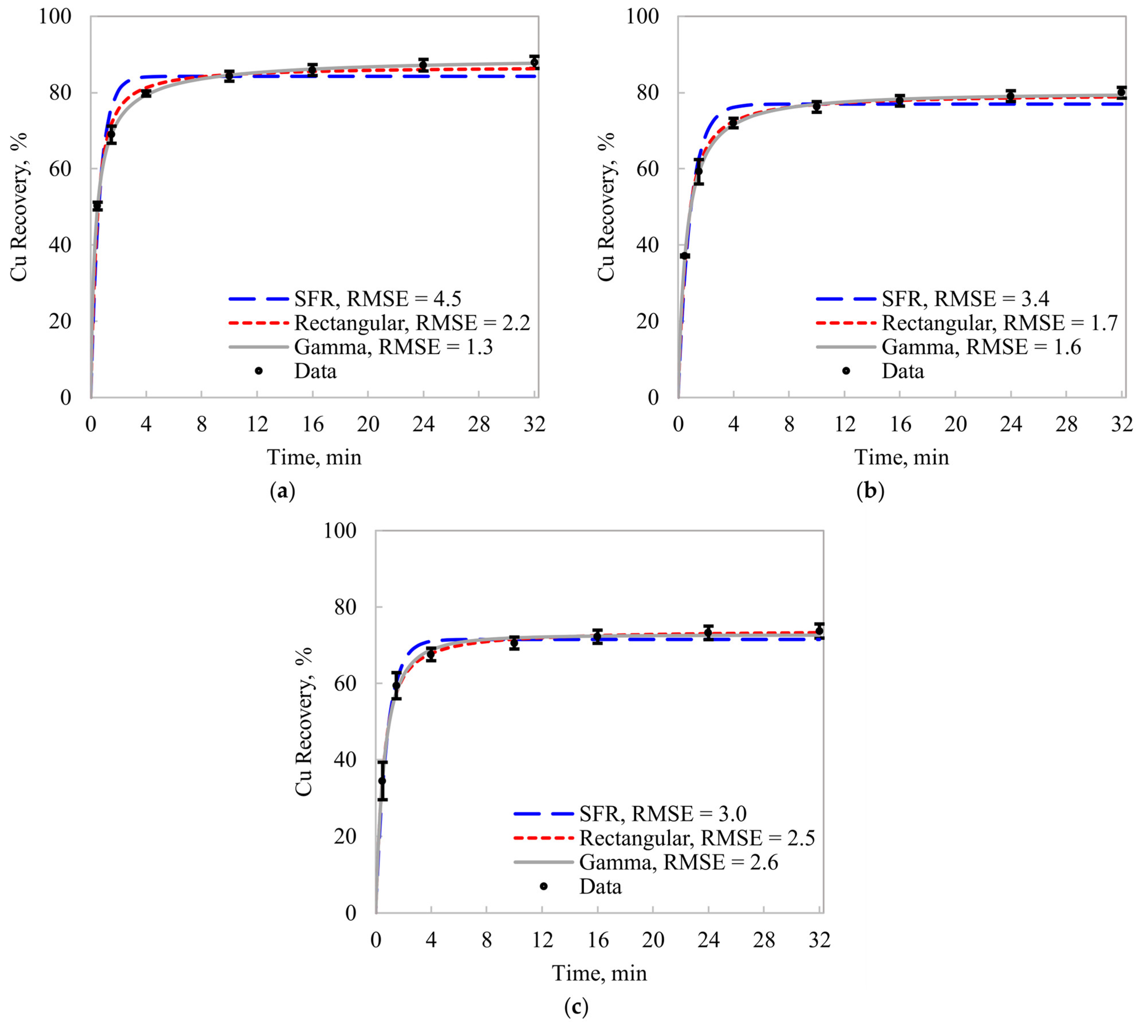
The R(t) models of Equations (1), (3), and (5) were fitted to the entire time-recovery datasets, from which reference R_∞–f(k) pairs were obtained (baseline kinetic parameters). Figure 2 shows the R(t) model fitting for the three evaluated experimental conditions (Figure 2a for P80 = 150 μm, Figure 2b for P80 = 212 μm, and Figure 2c for P80 = 300 μm), assuming the Single Flotation Rate, Rectangular, and Gamma models. The root mean squared errors (RMSEs) are presented as indicators of the magnitude of the modeling errors. The deterministic flotation rate of Equation (1) consistently led to the poorest kinetic representation for the experimental data.

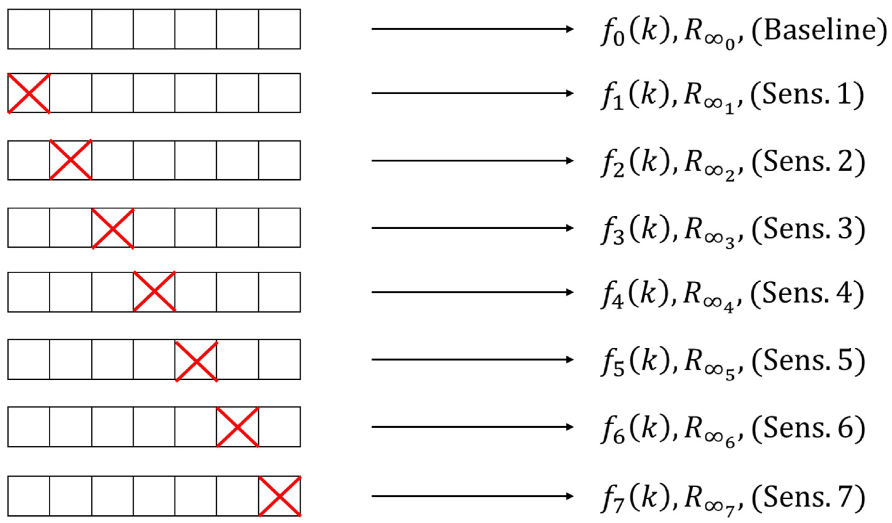
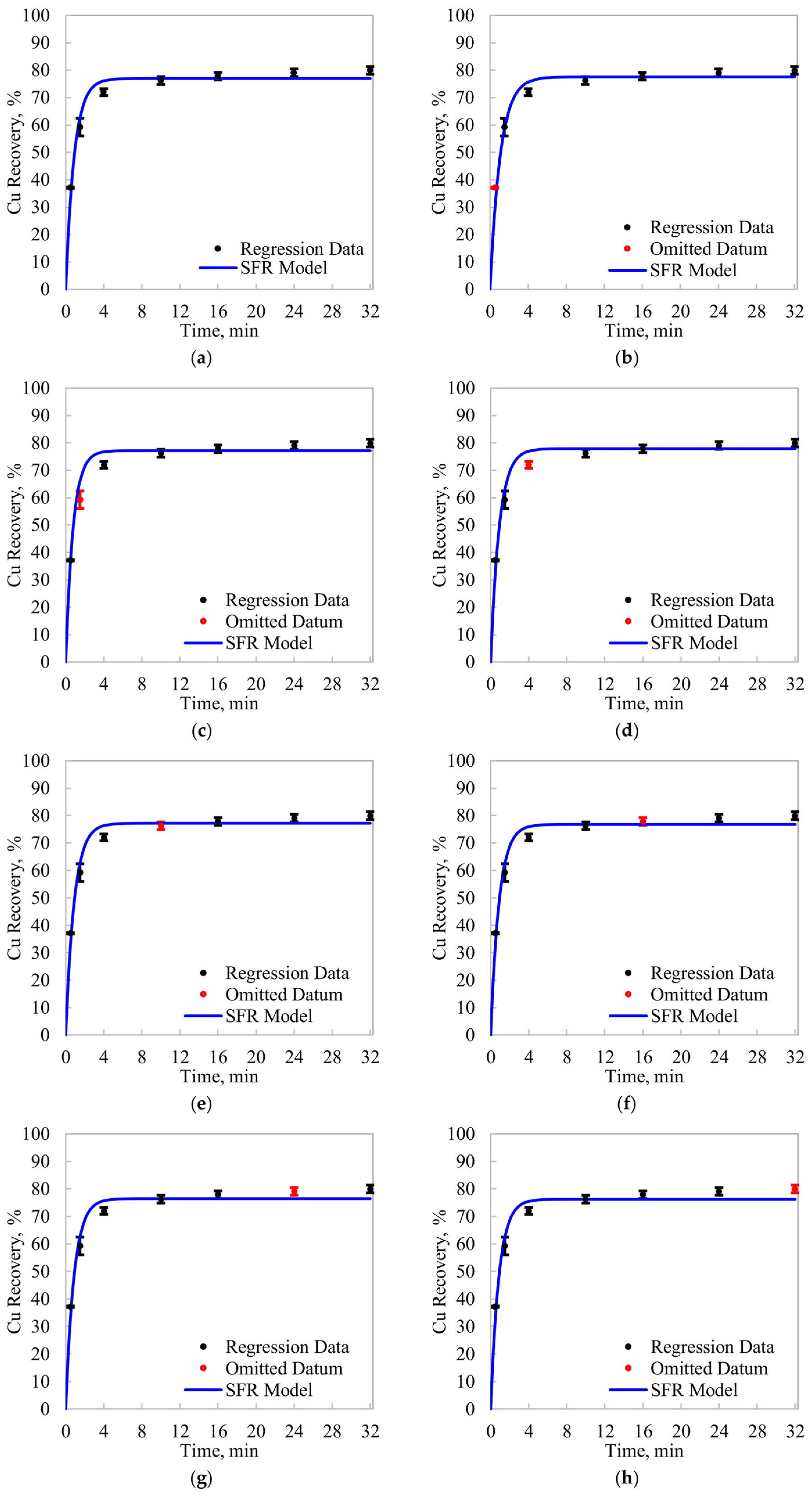
A sensitivity analysis was conducted using the procedure schematized in Figure 1. Figure 3 shows the model fitting, using the SFR model of Equation (1). Figure 3a presents the baseline condition, with no data removal. Figure 3b–h shows the model fitting after removing one datapoint at a time. From these results, the sensitivity of the R_∞–f(k) estimates under moderate changes in the flotation intervals was studied.

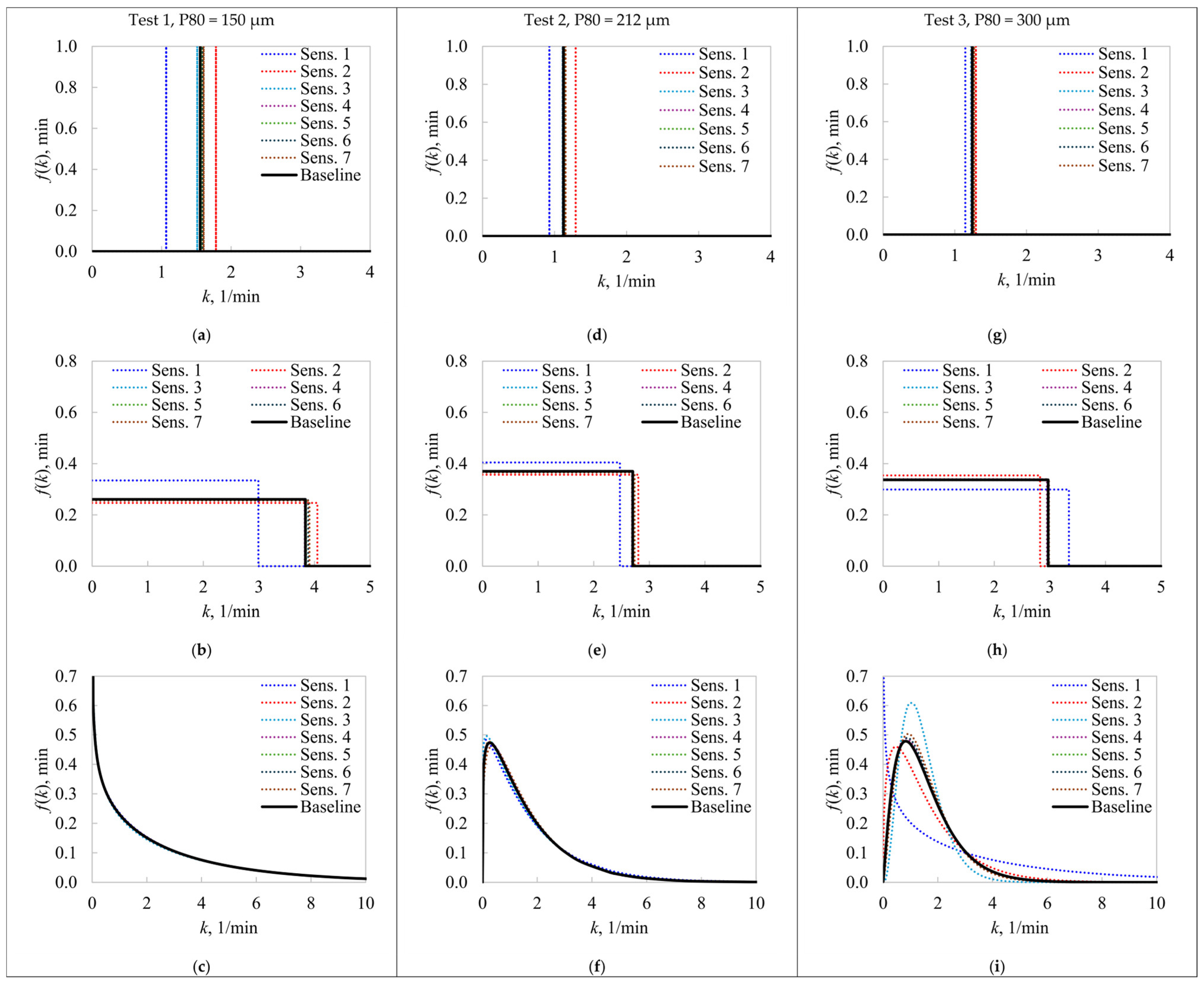
Figure 4 presents all the estimated f(k)s for the three evaluated experimental conditions. Figure 4a,d,g presents the estimated rate constants of the SFR model, Figure 4b,e,h the Rectangular f(k)s, and Figure 4c,f,i the Gamma f(k)s. The baseline f(k)s are shown as solid black lines, whereas the f(k)s from the sensitivity analysis are presented as colored dotted lines. In the plot legends, Sens. n indicates that the n-th datapoint was omitted in the parameter estimation, as shown in Figure 1.

The SFR and Rectangular models, in most cases, presented a high parameter sensitivity to the experimental design, specifically to the first two flotation intervals in the batch tests (Sens. 1 and Sens. 2). When individually omitting these datapoints, the k and k_max values [Equations (1) and (3), respectively] presented significant deviations regarding the baseline; however, Test 3 led to more robust estimates from the deterministic rate constant (Figure 4g). Removing time-recovery data from the third flotation interval did not lead to significant changes in the SFR and Rectangular f(k)s with respect to the baseline. Results for the SFR and Rectangular models indicate that using six datapoints in the kinetic tests will lead to uncertainties in the flotation rate parameters, particularly due to a poor characterization of the recovery rates at the beginning of the process. Thus, the results from Figure 4 suggest that additional flotation intervals must be included at short flotation times to guarantee more accurate k and k_max estimations. For Tests 1 and 2, the Gamma model of Equation (5) presented remarkably higher robustness compared to the SFR and Rectangular models. The location, dispersion, and shapes of these estimated f(k)s were not critically modified regarding the baseline. However, Test 3 led to unstable f(k) estimates from the Gamma model. This model has an additional parameter, which makes it more prone to overfitting, especially for noisy kinetic responses. Indeed, Figure 2c shows that the Gamma model presented poorer model fitting in Test 3, with respect to the first two experimental conditions. This result is mainly attributable to the higher variability of Test 3, as shown in the error bars of Figure 2 and Appendix A, and the higher flexibility of the Gamma model. As a result, removing the first datapoint significantly impacted the f(k) shape, and thus, the flotation rate characterization.

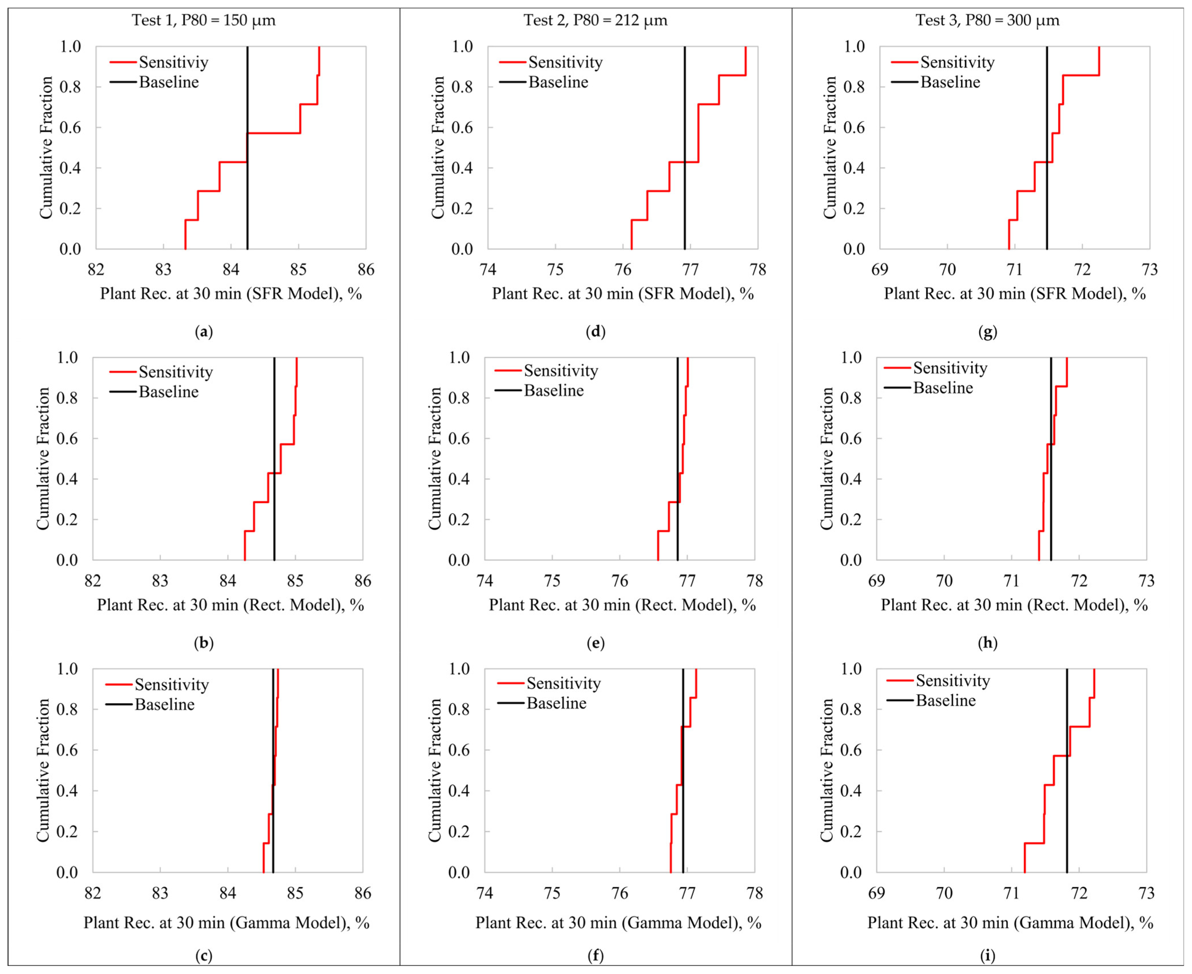
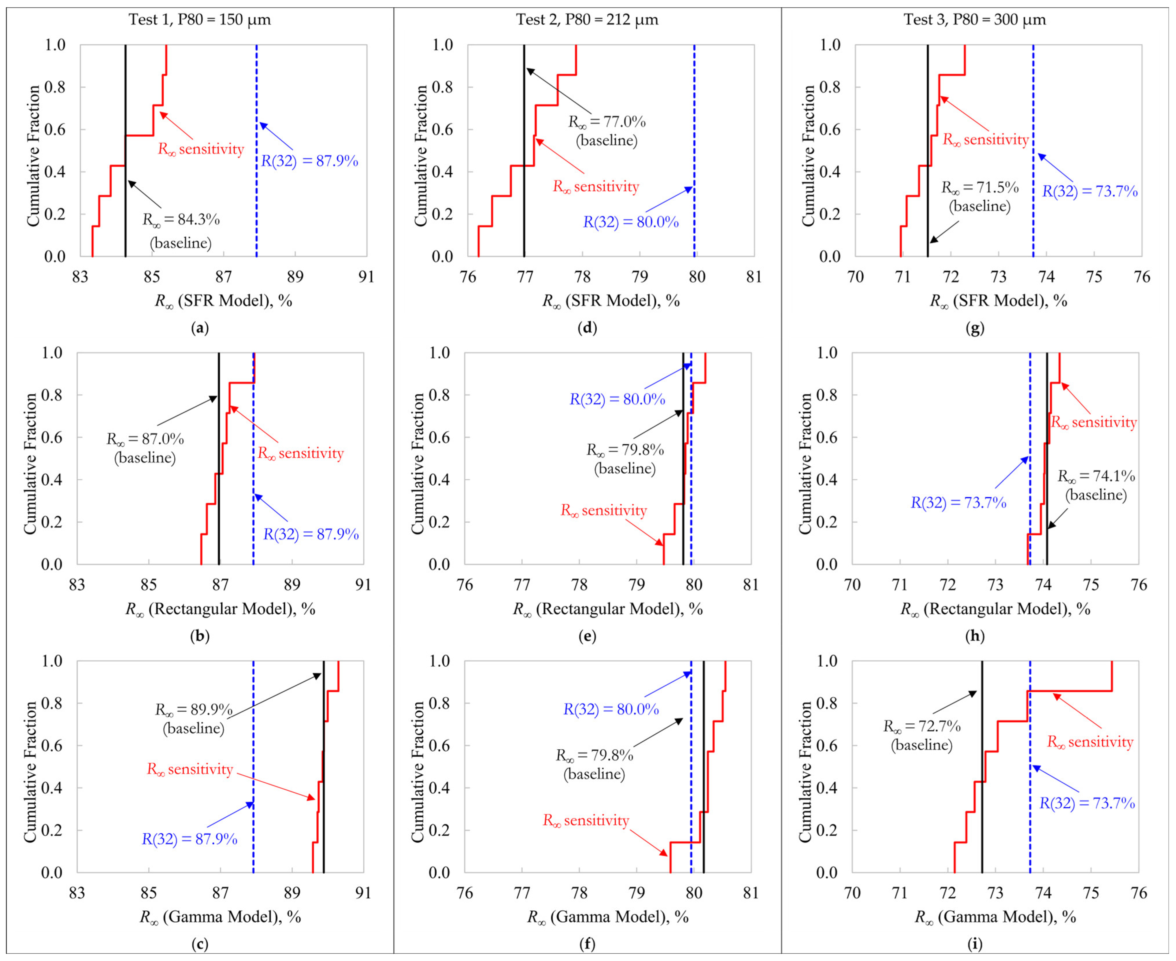
Figure 5 presents the variability in the R_∞ estimations when applying the sensitivity analysis, using the SFR (Figure 5a,d,g), Rectangular (Figure 5b,e,h), and Gamma (Figure 5c,f,i) models for the studied experimental conditions. The seven R_∞ estimates when removing one datapoint at a time are presented as cumulative distribution functions (cumulative fractions in red). The vertical continuous black lines represent the R_∞ values obtained in the baseline, with the entire dataset. As a reference, the measured cumulative recovery at t = 32 min [R(32)] is also deployed as a vertical blue line (dashed). In all cases, the SFR model led to R_∞ estimations significantly lower than the measured recovery at the end of the process, R(32). This inconsistency indicates the limitation of Equation (1) to characterize this flotation process. For Tests 1 and 2, the Rectangular model also led to R_∞ values lower than R(32); however, the differences are significantly lower than those observed with the SFR model. Similarly, the Gamma model presented inconsistencies in the R_∞ estimates with respect to the experimental data in Test 3, in agreement with the unstable f(k)s shown in Figure 4i. 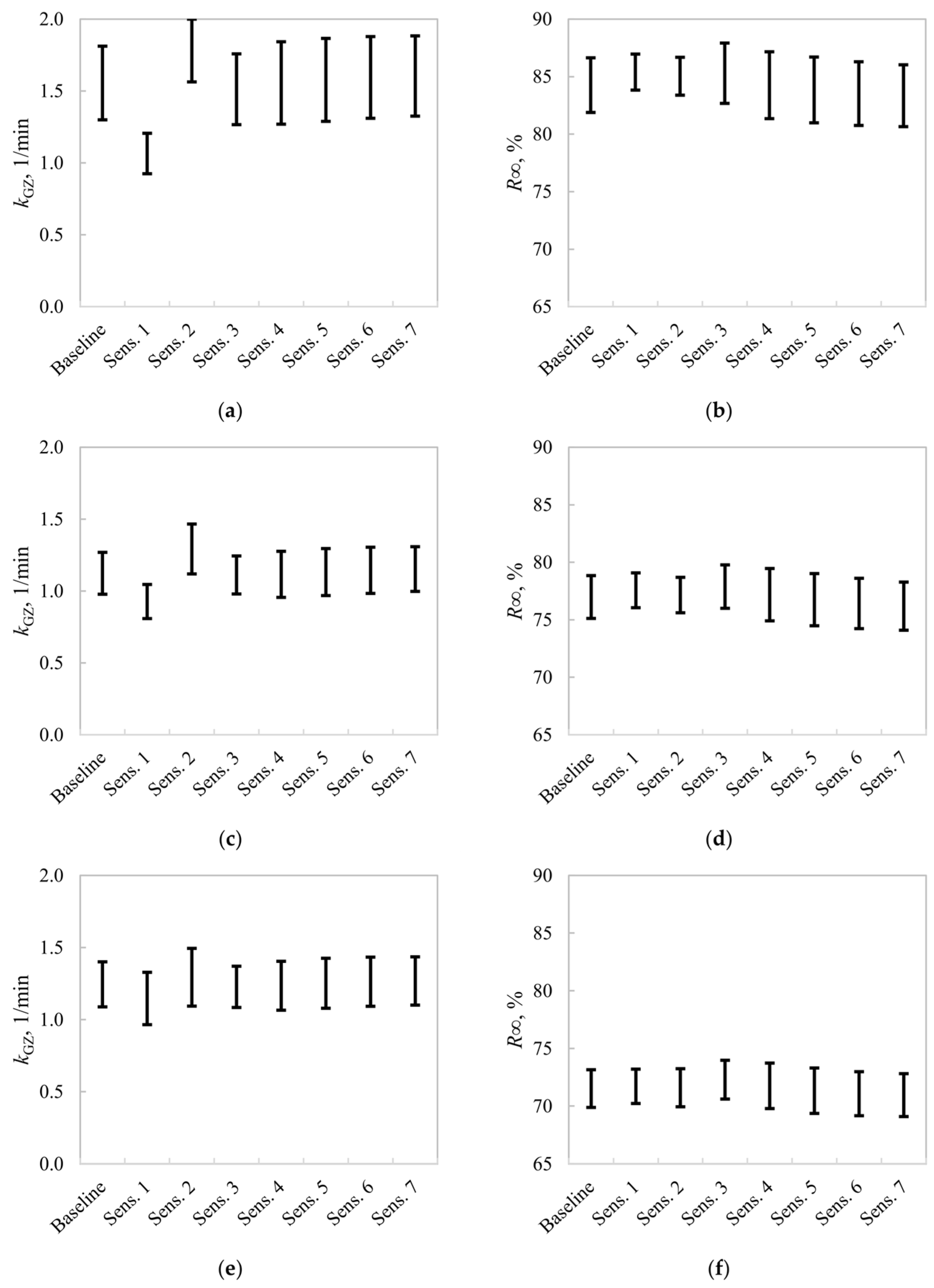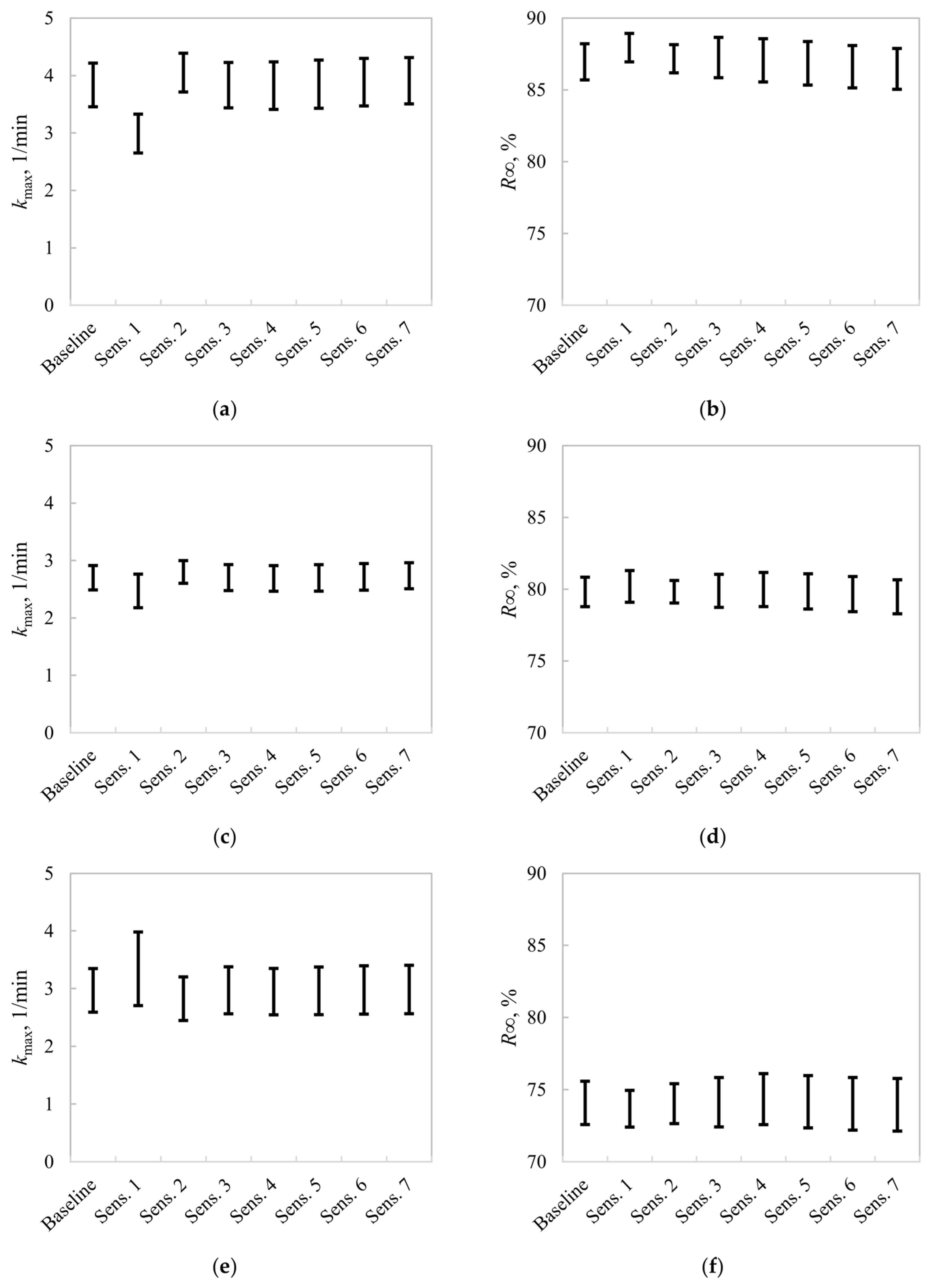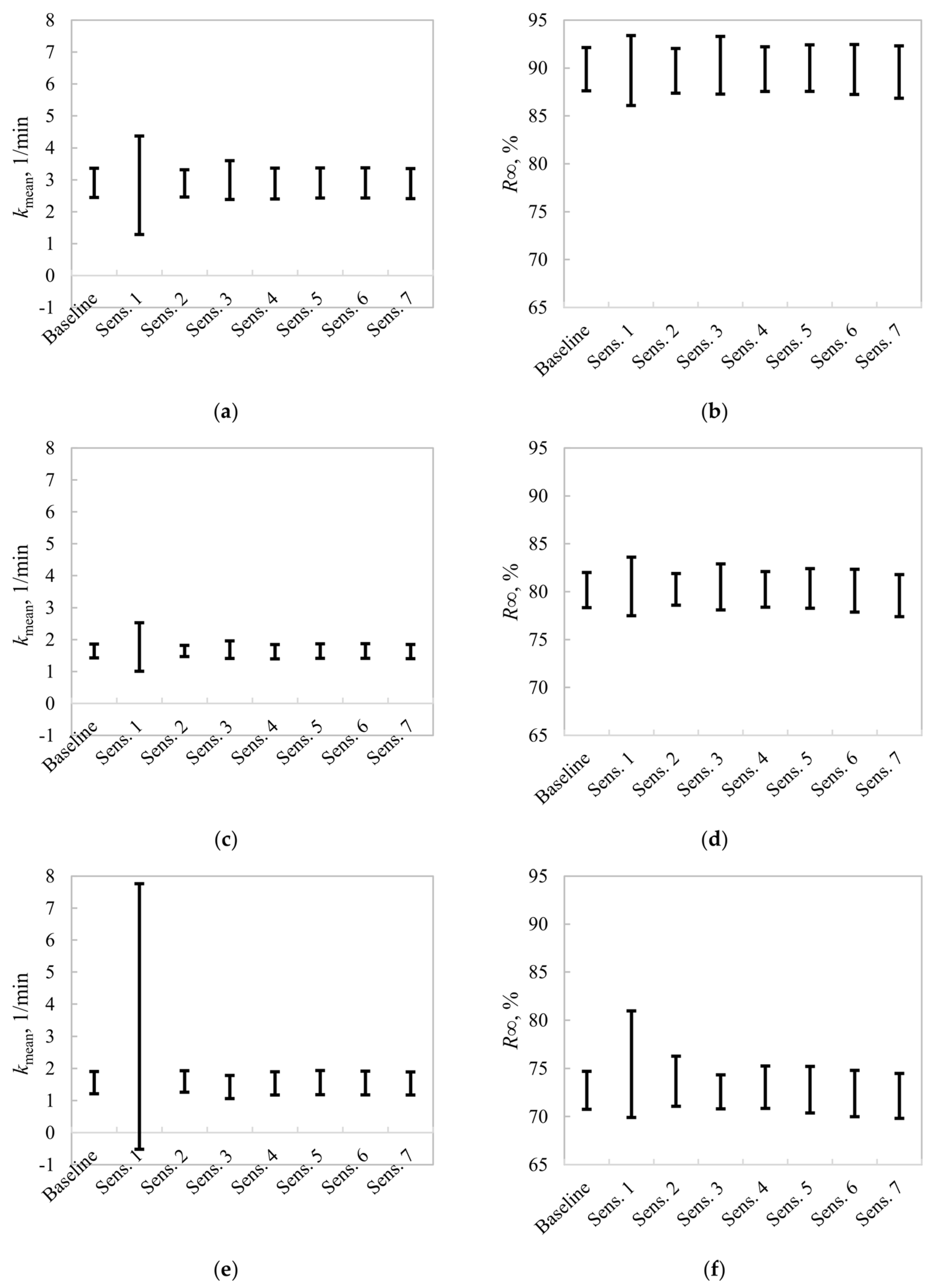Appendix B analyzed the 95% confidence intervals for all model parameters, from which similar patterns and uncertainties as those shown in Figure 4 and Figure 5 are observed for the estimations of R_∞ and the rate parameters. However, these intervals should be interpreted with caution, as some indications of heteroscedasticity are observed from Appendix A.

The SFR model consistently led to high variability in the R_∞ estimation. The comparative results between the Rectangular and Gamma models in terms of the R_∞ precision depended on the experimental conditions. In Test 1, the Gamma R_∞ estimations were more stable than those obtained from the Rectangular model. However, poor R_∞ estimations were obtained in Test 3 with the Gamma approach due to the noisier kinetic response and the higher flexibility of this model structure. In Test 2, the Rectangular model led to slightly lower R_∞ variability with respect to the Gamma model, though the maximum recovery values tended to be lower than the experimental recoveries at the end of the process.

An overall comparison of the kinetic representations states that the most robust approach in terms of the R_∞–f(k) stability depends on the experimental conditions. Test 1 was adequately described by the Gamma model, with negligible changes in the parameter estimation under moderate changes in the selection of flotation times. Test 3, on the other hand, had a more stable and consistent R_∞–f(k) estimation using the Rectangular model. Although both the Rectangular and Gamma models presented comparable results for Test 2, the more consistent R_∞ estimations with the experimental recoveries R(32) gave a slight advantage to the latter.

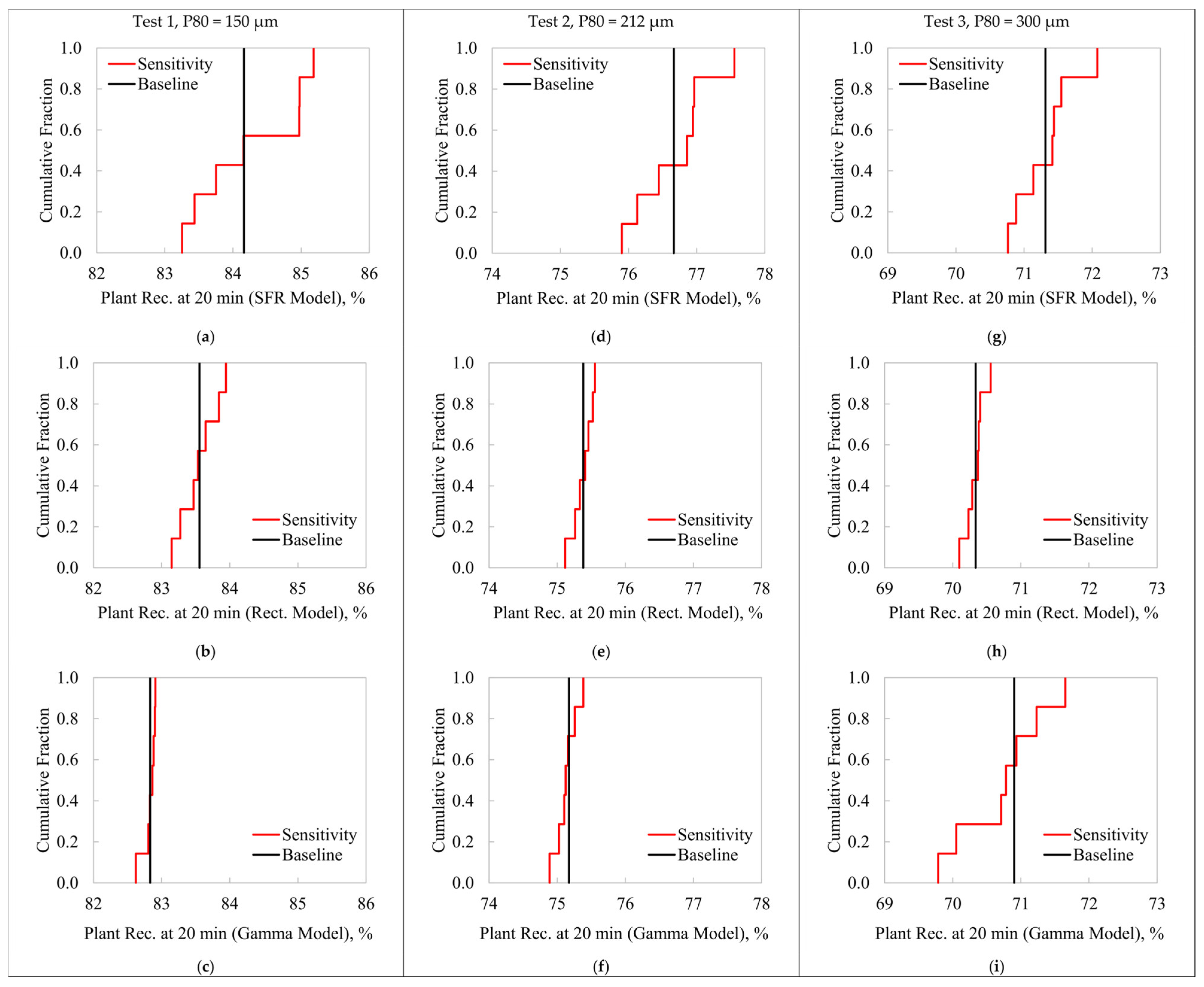
The R_∞–f(k) estimations of Figure 4 and Figure 5 were used to analyze the impact of the parameter uncertainties on the scale-up results, under moderate changes in the flotation intervals in the laboratory tests. For illustration purposes, six flotation cells in series were considered at large scale, in which each machine was assumed as a perfect mixer for the residence time distribution ξ(t) in Equation (6). A rougher circuit with a total flotation time of 20 min was evaluated, implying a mean residence time of 3.33 min per cell. A scale-up factor of 2.5 was used, as typically reported in literature [16]. Thus, for the SFR and Rectangular models, the rate parameters k/2.5 and k_max/2.5 were used when evaluating Equation (6). For the Gamma model, the mean rate constant was set to k_mean/2.5 at a large scale, keeping the same f(k) shapes as in Figure 4c,f,i. This assumption considers that a_G in Equation (4) did not change between the evaluated scales. It should be mentioned that the scale-up procedures assuming the SFR and Rectangular models are straightforward, as closed expressions for the large-scale recoveries can be obtained [17,29]. For the Gamma model, numerical integration is required.

Figure 6 presents the scale-up results at 20 min using the lab-scale kinetic characterizations in the baseline and from the sensitivity analysis, assuming the SFR (Figure 6a,d,g), Rectangular (Figure 6b,e,h), and Gamma (Figure 6c,f,i) models for the three feed P80s. All recoveries are presented as cumulative distribution functions. Figure A4 of Appendix C shows the same results for a large-scale residence time of 30 min, again considering six perfect mixers in series (mean residence time of 5.0 min per cell). The SFR model led to a high variability and high correlation with the maximum recoveries depicted in Figure 5a,d,g. As pure exponential trends rapidly converge to steady values, it is expected that scaling-up procedures with relatively long flotation times tend to R_∞. As these maximum recoveries were highly sensitive to the chosen flotation intervals in the laboratory tests, and their values were inconsistent with the experimental data, the SFR model structure is not recommended for scaling up this flotation process. Indeed, any flotation system presenting sustained increasing trends at long flotation times will not be well represented by Equation (1), discarding this model for scale-up purposes. It should be noted that the scaled-up SFR recoveries were significantly higher than those obtained from the Rectangular and Gamma models, again justified by the SFR convergence to the maximum recoveries. The uncertainties of the scaled-up recoveries when assuming the Rectangular and Gamma models agreed with the stabilities of the R_∞–f(k) estimates shown in Figure 4 and Figure 5. Thus, higher precision was obtained with the Gamma model in Test 1, and this trend was reversed in Test 3. In Test 2, comparable variability was obtained with both models, in agreement with the R_∞–f(k) uncertainties observed in Figure 4e,f and Figure 5e,f.

An alternative and simplified procedure considers the prediction of large-scale recoveries, scaling up the lab results based on the flotation times instead of the flotation rates. In this case, given a large-scale residence time τ, the predicted recovery is directly obtained from batch tests at t = τ/f, where f is a scale-up factor [16]. This scale-up factor has proven to be comparable to that from the ratio of batch/plant rate constants [30]. Thus, assuming an f value of 2.5, the large-scale recovery at 20 min can be estimated from the lab-scale recovery at 8 min. Using various interpolation techniques for the experimental data presented in Appendix A, the estimated recoveries of Tests 1, 2, and 3 at t = 8 min (τ = 20 min) were 83%, 75%, and 70%, respectively. These values are consistent with the estimated recoveries of Figure 6 for Tests 1 and 2 using the Rectangular and Gamma models, under moderate changes in the flotation intervals. For Test 3, only the Rectangular model led to a consistent estimation with respect to the interpolated recoveries. Again, the SFR model did not lead to recovery estimations that agree with the experimental data, showing the limited kinetic representation obtained from Equation (1).

The results presented here proved the sensitivity of kinetic characterizations to the selection of flotation intervals in laboratory tests. This sensitivity may critically affect the scale-up results for circuit sizing. Particularly, the SFR model not only presented poor model fitting, but also high R_∞–f(k) variability and inconsistent scale-up results. Therefore, this model structure is not recommended for flotation systems presenting slight increasing trends at long flotation times. The proposed methodology allows for the detection of opportunities for improvement in experimental design, detecting the sensitivity of the R_∞–f(k) pairs estimated from batch tests. It should be noted that the kinetic variability observed in Figure 4, Figure 5 and Figure 6 was only caused by the arbitrary selection of the flotation intervals in the batch tests, assuming unbiased sampling and that the operating conditions and ore properties were invariant. Thus, improvements in kinetic characterizations require decreasing the measurement noise and process disturbances, and designing experiments that reduce the error propagation to the model parameters.

From a practical point of view, the Rectangular model proved to be an adequate model structure for the evaluated ore, considering that there is a closed expression for the recovery at large scale (i.e., assuming perfect mixing). Only a moderate disadvantage with respect to the Gamma model was observed in Test 1, in terms of parameter stability and predictability. However, previous studies have shown that the goodness of a model structure cannot be generalizable to all flotation systems [31]. In any case, given a specific system, the methodology proposed in this work allows for the selection of kinetic models leading to a good trade-off between model fitting, parameter stability, and predictive capacity in flotation.

Some flotation processes and responses have inherently sustained increasing recoveries at the end of the tests, even for long flotation times. For example, in the separation of high-grade ores or when modeling non-selective recoveries (i.e., entrainment). In these cases, significant uncertainties in the R_∞ estimations are obtained as flotation kinetics do not reach a plateau at the end of the tests. Under this condition, the methodology proposed here will fail in detecting opportunities for improvement in the experimental design, as the limitation is fully justified by insufficient flotation time. Particularly, for non-selective separations, errors in gangue recoveries are critical for the prediction of concentrate grades, a subject that continues to be of interest among practitioners. Further developments are being made to establish a systematic procedure for a robust definition of flotation intervals in kinetic characterizations with the aim of determining the process evolution in terms of recovery and selectivity.

4. Conclusions

A sensitivity analysis was conducted for the characterization of flotation kinetics at laboratory scale. The time-recovery data was slightly modified, removing one datapoint at a time to assess the variability in the parameter estimation, assuming the Single Flotation Rate, Rectangular, and Gamma models. The stability of these estimates was used as an indicator of the robustness of the experimental design. The main findings are summarized as follows:

• The classical SFR model not only had poor model fitting but also led to high R_∞–k variability under moderate changes in the selection of flotation intervals in the laboratory tests. In addition, the R_∞ were consistently lower than the recoveries at the end of the process, given the abrupt decrease of pure exponential decays at long flotation times. As a result, this model structure was inadequate to scale up metallurgical results, as they converged to R_∞, with high variability.
• The Rectangular and Gamma models led to more stable kinetic characterizations. However, the latter also presented high R_∞–f(k) uncertainties at a feed P80 = 300 µm, which was attributed to the potential overfitting under noisy kinetic responses. The parameter stability depended on the experimental conditions. At P80 = 150 µm, the Gamma model led to the highest stability for the R_∞–f(k) estimates, whereas at P80 = 300 µm, the best results were obtained with the Rectangular approach. At P80 = 212 µm, non-significant differences were obtained with both models, with a slight advantage from the Gamma model due to the consistency between the estimated R_∞ and the recovery at the end of the process.
• For scaling-up metallurgical results, the Rectangular and Gamma models kept the same patterns in terms of stability as those of the kinetic parameters. An important feature of both kinetic representations was their consistency with the simplified scale-up approach by flotation/residence time. This consistency was not observed with the classical SFR model, indicating again the poor results typically obtained when assuming pure exponential decays.

The sensitivity analysis presented here proved the significant impact of the selected flotation intervals on kinetic characterizations. As these intervals are, in most cases, arbitrarily chosen in laboratory tests, these findings illustrate the relevance of running optimal experimental designs to minimize R_∞–f(k) uncertainties. Further developments are being made to systematically improve kinetic modeling in flotation.